

Real-Time Machine Learning-Based Driver Drowsiness Detection Using Visual Features


Abstract
1. Introduction
2. Related Work
3. Methodology
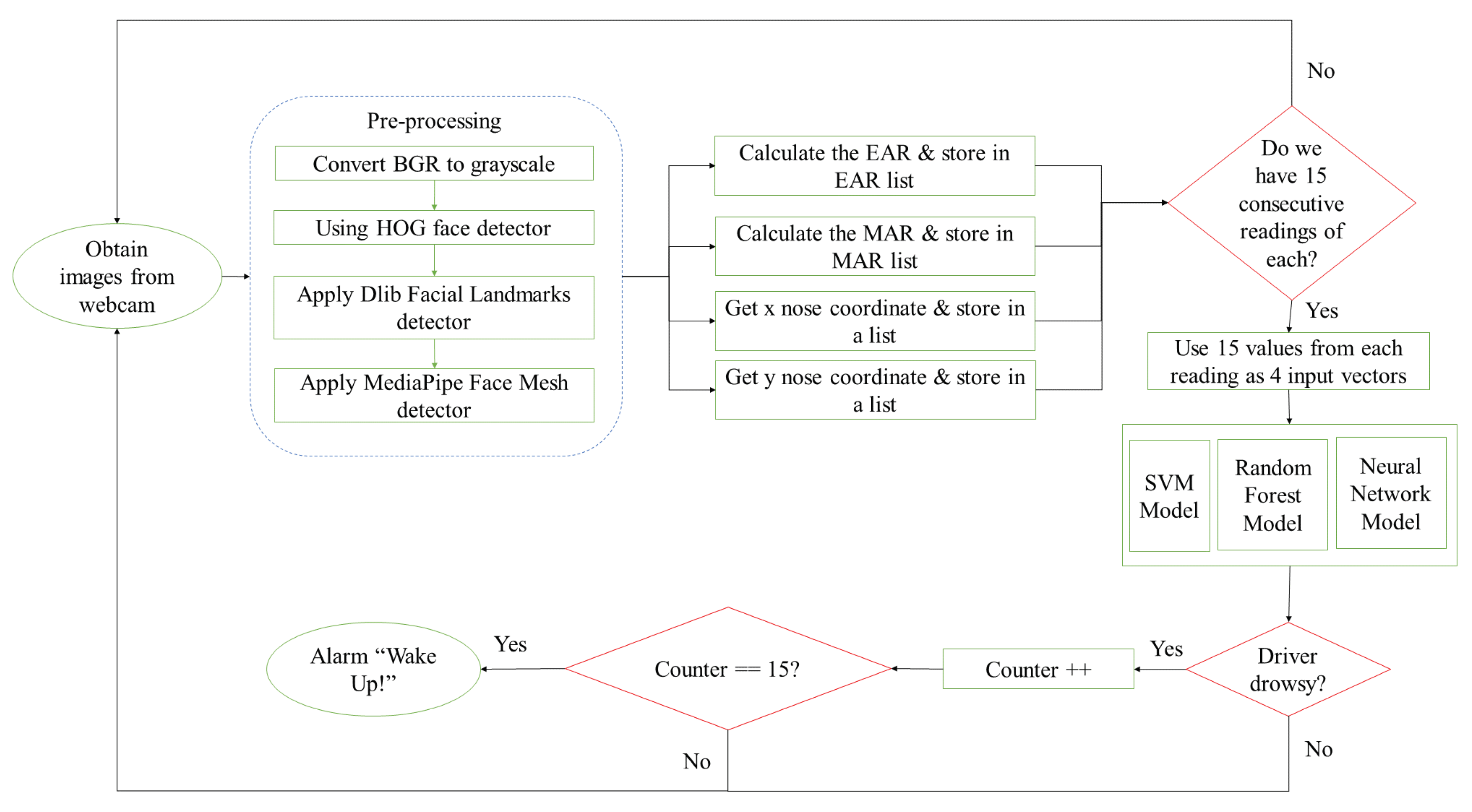
3.1. System Design
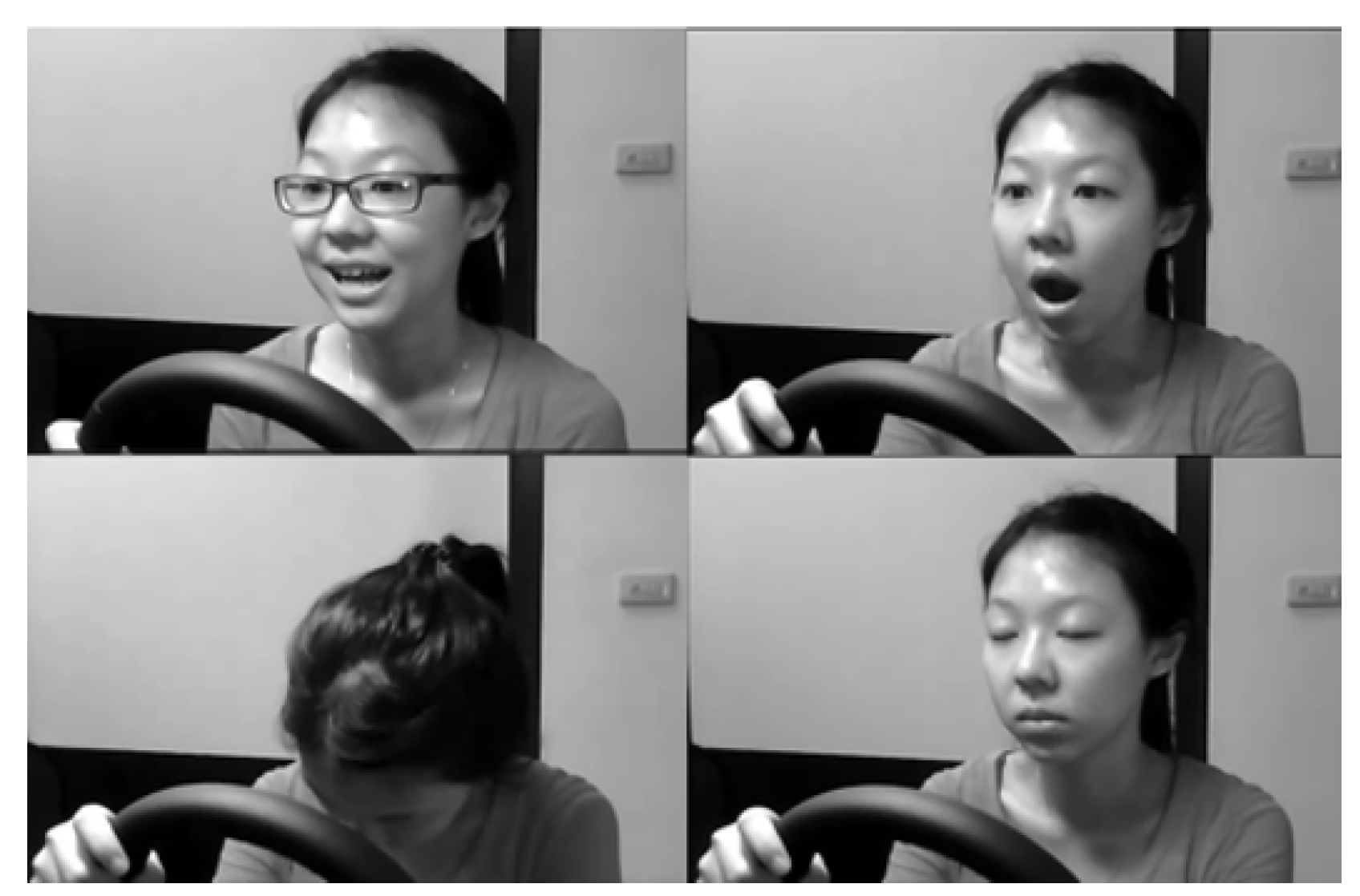
3.2. Dataset
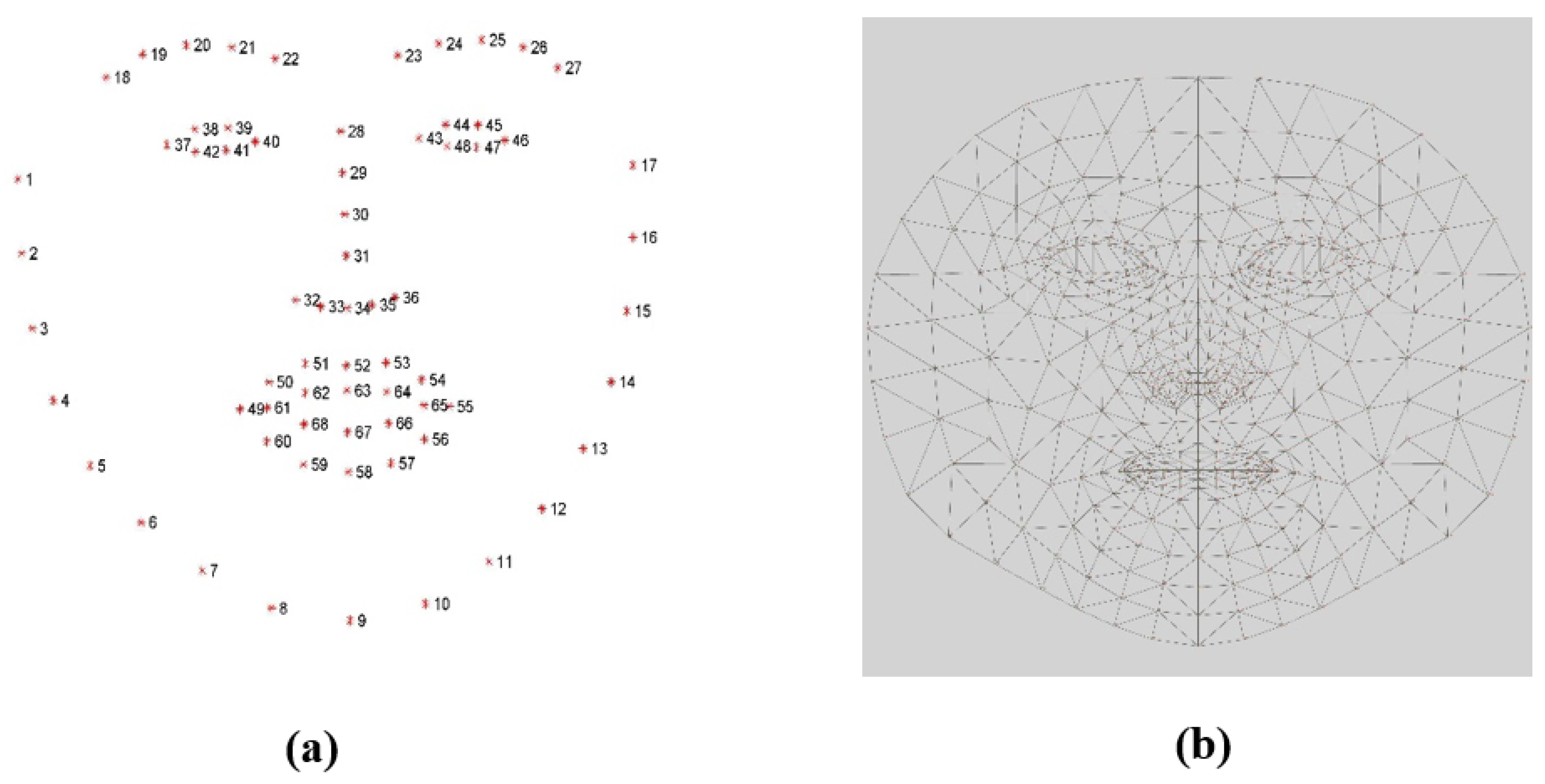
3.3. Preprocessing
3.4. Feature Extraction
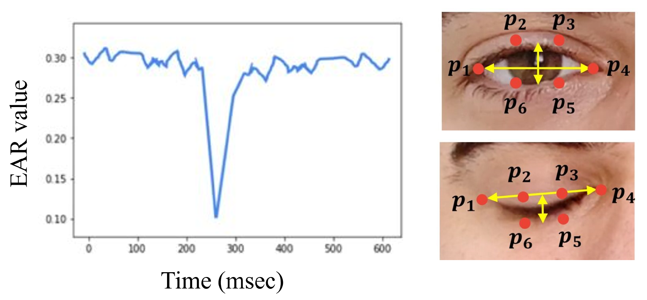
3.4.1. EAR Metric
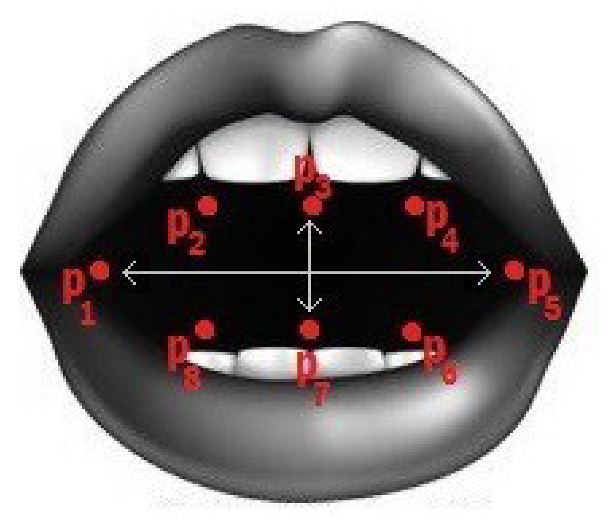
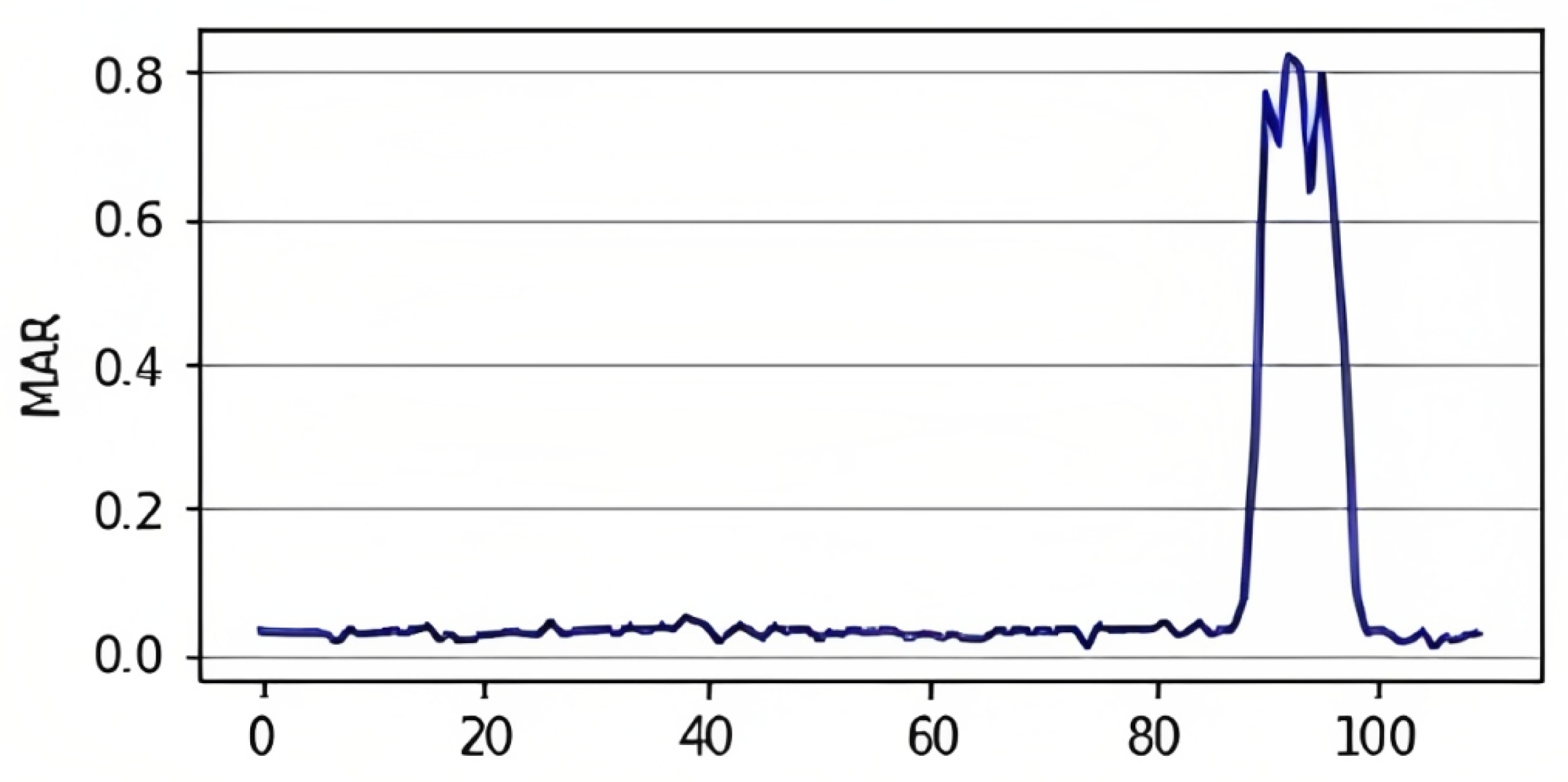
3.4.2. MAR Metric
3.4.3. Drowsy Head Pose
- Head pose up, if X of angle 7
- Head pose down, if X of angle −7
- Head pose right, if Y of angle 7
- Head pose left, if Y of angle −7
3.5. Data Labeling
3.6. Classification
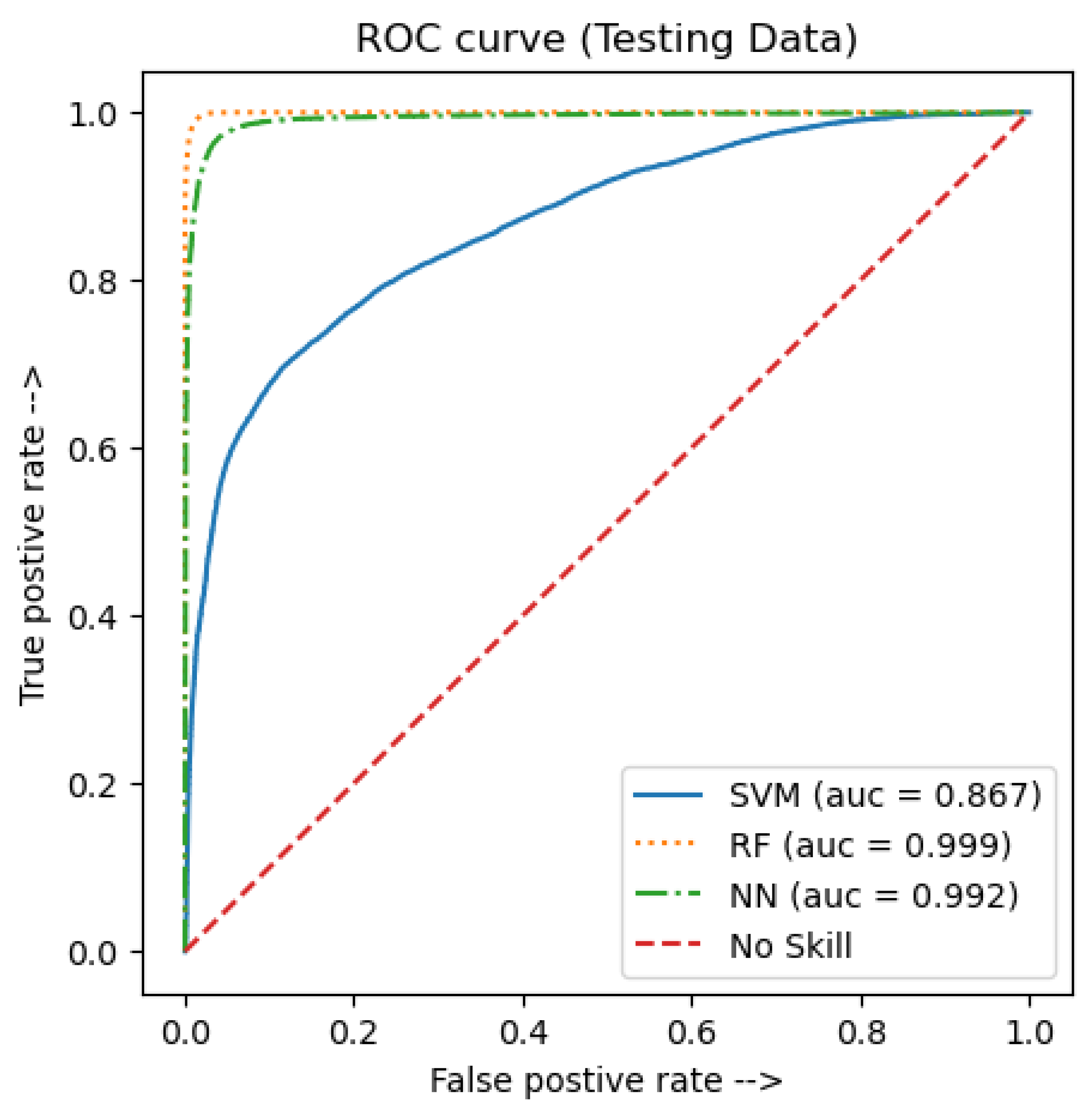
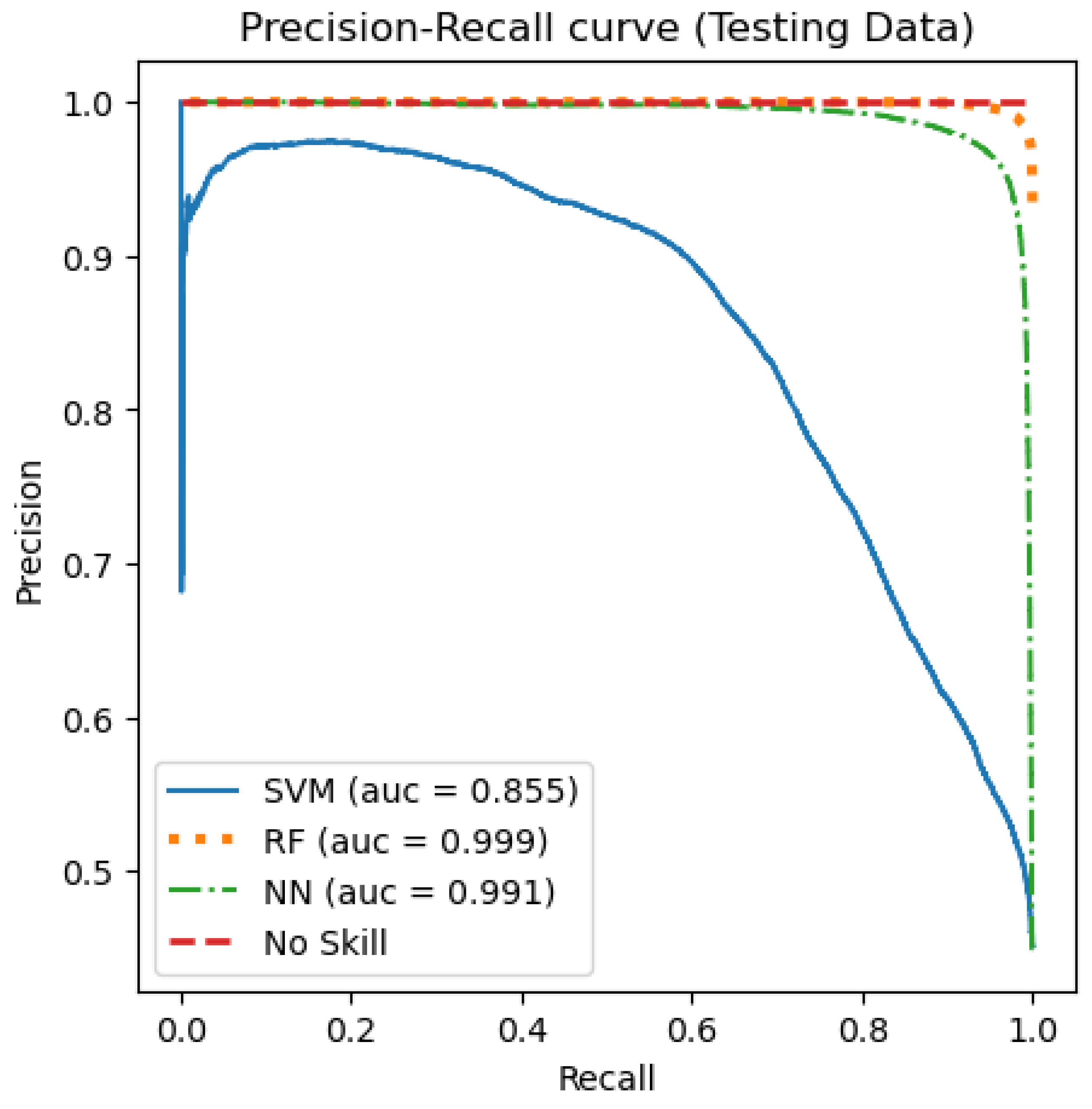
4. Results and Discussion
5. Conclusions
Author Contributions
Funding
Institutional Review Board Statement
Informed Consent Statement
Data Availability Statement
Conflicts of Interest
Abbreviations
| DDD | Driver Drowsiness Detection |
| EEG | electroencephalography |
| ECG | electrocardiography |
| EMG | electromyography |
| EOG | electrooculography |
| RF | Random Forest |
| NN | Neural Networks |
| SVM | Support Vector Machine |
| BGR | Blue Green Red |
| EAR | Eye Aspect Ratio |
| MAR | Mouth Aspect Ratio |
| NTHUDDD | National Tsing HuaUniversity DDD |
| CNN | Convolutional Neural Networks |
| HOG | Histogram of Oriented Gradients |
| ROC | Receiver Operating Characteristic |
| AUC | Area Under the Curve |
References
- Al Amir, S. Road Accidents in UAE Caused 381 Deaths Last Year. Available online: https://www.thenationalnews.com (accessed on 10 December 2022).
- Albadawi, Y.; Takruri, M.; Awad, M. A review of recent developments in driver drowsiness detection systems. Sensors 2022, 22, 2069. [Google Scholar] [CrossRef] [PubMed]
- Ramzan, M.; Khan, H.U.; Awan, S.M.; Ismail, A.; Ilyas, M.; Mahmood, A. A survey on state-of-the-art drowsiness detection techniques. IEEE Access 2019, 7, 61904–61919. [Google Scholar] [CrossRef]
- Sikander, G.; Anwar, S. Driver fatigue detection systems: A review. IEEE Trans. Intell. Transp. Syst. 2018, 20, 2339–2352. [Google Scholar] [CrossRef]
- Pratama, B.G.; Ardiyanto, I.; Adji, T.B. A review on driver drowsiness based on image, bio-signal, and driver behavior. In Proceedings of the IEEE 2017 3rd International Conference on Science and Technology-Computer (ICST), Yogyakarta, Indonesia, 11–12 July 2017; pp. 70–75. [Google Scholar]
- Kaur, R.; Singh, K. Drowsiness detection based on EEG signal analysis using EMD and trained neural network. Int. J. Sci. Res. 2013, 10, 157–161. [Google Scholar]
- Kundinger, T.; Sofra, N.; Riener, A. Assessment of the potential of wrist-worn wearable sensors for driver drowsiness detection. Sensors 2020, 20, 1029. [Google Scholar] [CrossRef]
- Sahayadhas, A.; Sundaraj, K.; Murugappan, M.; Palaniappan, R. Physiological signal based detection of driver hypovigilance using higher order spectra. Expert Syst. Appl. 2015, 42, 8669–8677. [Google Scholar] [CrossRef]
- Khushaba, R.N.; Kodagoda, S.; Lal, S.; Dissanayake, G. Driver drowsiness classification using fuzzy wavelet-packet-based feature-extraction algorithm. IEEE Trans. Biomed. Eng. 2010, 58, 121–131. [Google Scholar] [CrossRef]
- McDonald, A.D.; Schwarz, C.; Lee, J.D.; Brown, T.L. Real-time detection of drowsiness related lane departures using steering wheel angle. In Proceedings of the Human Factors and Ergonomics Society Annual Meeting; Sage Publications: Los Angeles, CA, USA, 2012; Volume 56, pp. 2201–2205. [Google Scholar]
- Ma, J.; Murphey, Y.L.; Zhao, H. Real time drowsiness detection based on lateral distance using wavelet transform and neural network. In Proceedings of the 2015 IEEE Symposium Series on Computational Intelligence, Cape Town, South Africa, 7–10 December 2015; pp. 411–418. [Google Scholar]
- Kiashari, S.E.H.; Nahvi, A.; Bakhoda, H.; Homayounfard, A.; Tashakori, M. Evaluation of driver drowsiness using respiration analysis by thermal imaging on a driving simulator. Multimed. Tools Appl. 2020, 79, 17793–17815. [Google Scholar] [CrossRef]
- Bamidele, A.A.; Kamardin, K.; Abd Aziz, N.S.N.; Sam, S.M.; Ahmed, I.S.; Azizan, A.; Bani, N.A.; Kaidi, H.M. Non-intrusive driver drowsiness detection based on face and eye tracking. Int. J. Adv. Comput. Sci. Appl. 2019, 10. [Google Scholar] [CrossRef]
- Khunpisuth, O.; Chotchinasri, T.; Koschakosai, V.; Hnoohom, N. Driver drowsiness detection using eye-closeness detection. In Proceedings of the 2016 12th International Conference on Signal-Image Technology & Internet-Based Systems (SITIS), Naples, Italy, 28 November–1 December 2016; pp. 661–668. [Google Scholar]
- Triyanti, V.; Iridiastadi, H. Challenges in detecting drowsiness based on driver’s behavior. IOP Conf. Ser. Mater. Sci. Eng. 2017, 277, 012042. [Google Scholar] [CrossRef]
- Knapik, M.; Cyganek, B. Driver’s fatigue recognition based on yawn detection in thermal images. Neurocomputing 2019, 338, 274–292. [Google Scholar] [CrossRef]
- Tayab Khan, M.; Anwar, H.; Ullah, F.; Ur Rehman, A.; Ullah, R.; Iqbal, A.; Lee, B.H.; Kwak, K.S. Smart real-time video surveillance platform for drowsiness detection based on eyelid closure. Wirel. Commun. Mob. Comput. 2019, 2019, 2036818. [Google Scholar] [CrossRef]
- Lin, S.T.; Tan, Y.Y.; Chua, P.Y.; Tey, L.K.; Ang, C.H. Perclos threshold for drowsiness detection during real driving. J. Vis. 2012, 12, 546. [Google Scholar] [CrossRef]
- Rosebrock, A. Eye Blink Detection with Opencv, Python, and Dlib. Available online: https://pyimagesearch.com/2017/04/24/eye-blink-detection-opencv-python-dlib/ (accessed on 7 May 2022).
- Moujahid, A.; Dornaika, F.; Arganda-Carreras, I.; Reta, J. Efficient and compact face descriptor for driver drowsiness detection. Expert Syst. Appl. 2021, 168, 114334. [Google Scholar] [CrossRef]
- Sri Mounika, T.; Phanindra, P.; Sai Charan, N.; Kranthi Kumar Reddy, Y.; Govindu, S. Driver Drowsiness Detection Using Eye Aspect Ratio (EAR), Mouth Aspect Ratio (MAR), and Driver Distraction Using Head Pose Estimation. In ICT Systems and Sustainability; Springer: Berlin/Heidelberg, Germany, 2022; pp. 619–627. [Google Scholar]
- Celecia, A.; Figueiredo, K.; Vellasco, M.; González, R. A portable fuzzy driver drowsiness estimation system. Sensors 2020, 20, 4093. [Google Scholar] [CrossRef] [PubMed]
- Popieul, J.C.; Simon, P.; Loslever, P. Using driver’s head movements evolution as a drowsiness indicator. In Proceedings of the IEEE IV2003 Intelligent Vehicles Symposium. Proceedings (Cat. No. 03TH8683), Columbus, OH, USA, 9–11 June 2003; pp. 616–621. [Google Scholar]
- Coetzer, R.; Hancke, G. Driver fatigue detection: A survey. In Proceedings of the AFRICON 2009, Nairobi, Kenya, 23–25 September 2009; pp. 1–6. [Google Scholar]
- Liu, W.; Qian, J.; Yao, Z.; Jiao, X.; Pan, J. Convolutional two-stream network using multi-facial feature fusion for driver fatigue detection. Future Internet 2019, 11, 115. [Google Scholar] [CrossRef]
- Soukupova, T.; Cech, J. Eye blink detection using facial landmarks. In Proceedings of the 21st Computer Vision Winter Workshop, Rimske Toplice, Slovenia, 3–5 February 2016. [Google Scholar]
- Maior, C.B.S.; das Chagas Moura, M.J.; Santana, J.M.M.; Lins, I.D. Real-time classification for autonomous drowsiness detection using eye aspect ratio. Expert Syst. Appl. 2020, 158, 113505. [Google Scholar] [CrossRef]
- Al Redhaei, A.; Albadawi, Y.; Mohamed, S.; Alnoman, A. Realtime Driver Drowsiness Detection Using Machine Learning. In Proceedings of the 2022 Advances in Science and Engineering Technology International Conferences (ASET), Dubai, United Arab Emirates, 21–24 February 2022; pp. 1–6. [Google Scholar]
- Rasna, P.; Smithamol, M. SVM-Based Drivers Drowsiness Detection Using Machine Learning and Image Processing Techniques. In Progress in Advanced Computing and Intelligent Engineering; Springer: Berlin/Heidelberg, Germany, 2021; pp. 100–112. [Google Scholar]
- Saradadevi, M.; Bajaj, P. Driver fatigue detection using mouth and yawning analysis. Int. J. Comput. Sci. Netw. Secur. 2008, 8, 183–188. [Google Scholar]
- Sahayadhas, A.; Sundaraj, K.; Murugappan, M. Detecting driver drowsiness based on sensors: A review. Sensors 2012, 12, 16937–16953. [Google Scholar] [CrossRef]
- Ngxande, M.; Tapamo, J.R.; Burke, M. Driver drowsiness detection using behavioral measures and machine learning techniques: A review of state-of-art techniques. In Proceedings of the 2017 Pattern Recognition Association of South Africa and Robotics and Mechatronics (PRASA-RobMech), Loemfontein, South Africa, 30 November–1 December 2017; pp. 156–161. [Google Scholar]
- Dwivedi, K.; Biswaranjan, K.; Sethi, A. Drowsy driver detection using representation learning. In Proceedings of the 2014 IEEE International Advance Computing Conference (IACC), Gurgaon, India, 21–22 February 2014; pp. 995–999. [Google Scholar]
- Dua, M.; Singla, R.; Raj, S.; Jangra, A.; Shakshi. Deep CNN models-based ensemble approach to driver drowsiness detection. Neural Comput. Appl. 2021, 33, 3155–3168. [Google Scholar] [CrossRef]
- Rosebrock, A. Face Detection with Dlib (Hog and CNN). Available online: https://pyimagesearch.com/2021/04/19/face-detection-with-dlib-hog-and-cnn/ (accessed on 7 May 2022).
- Kartynnik, Y.; Ablavatski, A.; Grishchenko, I.; Grundmann, M. Real-time facial surface geometry from monocular video on mobile GPUs. arXiv 2019, arXiv:1907.06724. [Google Scholar]
- Weng, C.H.; Lai, Y.H.; Lai, S.H. Driver drowsiness detection via a hierarchical temporal deep belief network. In Proceedings of the Asian Conference on Computer Vision; Springer: Berlin/Heidelberg, Germany, 2016; pp. 117–133. [Google Scholar]
- Datahacker. How to Detect Eye Blinking in Videos Using Dlib and Opencv in Python. Available online: https://datahacker.rs/011-how-to-detect-eye-blinking-in-videos-using-dlib-and-opencv-in-python/ (accessed on 20 May 2022).
- Cech, J.; Soukupova, T. Real-Time Eye Blink Detection Using Facial Landmarks; Center for Machine Perception, Department of Cybernetics. Faculty of Electrical Engineering, Czech Technical University in Prague: Prague, Czech Republic, 2016; pp. 1–8. [Google Scholar]
- Bhesal, A.D.; Khan, F.A.; Kadam, V.S. Motion based cursor for Phocomelia Users. Int. J. Emerg. Technol. Innov. Res. 2022, 9, 293–297. [Google Scholar]
- Taschenbuch Verlag Schiffman, H. Sensation and Perception: An Integrated Approach; John Wiley & Sons, Inc.: New York, NY, USA, 2001. [Google Scholar]
- Maior, C.B.S.; Moura, M.C.; de Santana, J.; do Nascimento, L.M.; Macedo, J.B.; Lins, I.D.; Droguett, E.L. Real-time SVM classification for drowsiness detection using eye aspect ratio. In Proceedings of the Probabilistic Safety Assessment and Management PSAM 14, Los Angeles, CA, USA, 16–21 September 2018. [Google Scholar]
- Keras Team, Keras Documentation: The Sequential Model. Available online: https://keras.io/guides/sequential_model/ (accessed on 15 March 2022).
- Breiman, L. Random forests. Mach. Learn. 2001, 45, 5–32. [Google Scholar] [CrossRef]
- Scikit-Learn. 1.4. Support Vector Machines. Available online: https://scikit-learn.org/stable/modules/svm.html (accessed on 22 March 2022).
- Brownlee, J. How to Use ROC Curves and Precision-Recall Curves for Classification in Python. Available online: https://machinelearningmastery.com/roc-curves-and-precision-recall-curves-for-classification-in-python/ (accessed on 28 March 2022).
- Kumar, A.; Patra, R. Driver drowsiness monitoring system using visual behaviour and machine learning. In Proceedings of the 2018 IEEE Symposium on Computer Applications & Industrial Electronics (ISCAIE), Penang, Malaysia, 28–29 April 2018; pp. 339–344. [Google Scholar]
- Chirra, V.R.R.; Uyyala, S.R.; Kolli, V.K.K. Deep CNN: A Machine Learning Approach for Driver Drowsiness Detection Based on Eye State. Rev. D’Intell. Artif. 2019, 33, 461–466. [Google Scholar] [CrossRef]
- Yu, J.; Park, S.; Lee, S.; Jeon, M. Driver Drowsiness Detection Using Condition-Adaptive Representation Learning Framework. IEEE Trans. Intell. Transp. Syst. 2019, 20, 4206–4218. [Google Scholar] [CrossRef]
- Fatima, B.; Shahid, A.R.; Ziauddin, S.; Safi, A.A.; Ramzan, H. Driver fatigue detection using viola jones and principal component analysis. Appl. Artif. Intell. 2020, 34, 456–483. [Google Scholar] [CrossRef]
- Ed-doughmi, Y.; Idrissi, N.; Hbali, Y. Real-Time System for Driver Fatigue Detection Based on a Recurrent Neuronal Network. J. Imaging 2020, 6, 8. [Google Scholar] [CrossRef]
- Sheikh, A.A.; Mir, J. Machine Learning Inspired Vision-based Drowsiness Detection using Eye and Body Motion Features. In Proceedings of the 2021 13th International Conference on Information & Communication Technology and System (ICTS), Surabaya, Indonesia, 20–21 October 2021; pp. 146–150. [Google Scholar] [CrossRef]


| Driver’s Behaviors | Description |
|---|---|
| Looking aside | When the head turns left or right |
| Talking and laughing | When talking or laughing |
| Sleepy-eyes | When eyes slowly close due to drowsiness |
| Yawning | When mouth open wide due to drowsiness |
| Nodding | When head falls forward when drowsy |
| Drowsy | When the driver visually looks sleepy, showing signs such as slowly blinking, yawning, and nodding |
| Stillness | When normally driving |
| Videos | Description |
| yawning.avi | Contains yawning behavior |
| sleepyCombination.avi | Contains a combination of drowsy behaviors (nodding, slow eye blinking, and yawning) |
| slowBlinkWithNodding.avi | Contains slow eye blinking and head nodding behavior |
| nonsleepyCombination.avi | Contains a combination of non-drowsy behaviors talking, laughing, looking aside |
| Temporal Window Size | Training Instances Labeled Drowsy in Subject 1 | Training Instances Labeled Drowsy in Subject 2 | Training instances Labeled Drowsy in Subject 3 |
|---|---|---|---|
| 9 | 2964 | 2218 | 3924 |
| 13 | 2851 | 2111 | 3802 |
| 15 | 2800 | 2057 | 3768 |
| 17 | 2739 | 2010 | 3714 |
| 21 | 2645 | 1922 | 3655 |
| Subject Number | Max EAR | Max MAR |
|---|---|---|
| 1 | 0.36 | 0.75 |
| 2 | 0.36 | 0.9 |
| 3 | 0.23 | 0.9 |
| 4 | 0.34 | 0.9 |
| 5 | 0.36 | 0.9 |
| 6 | 0.34 | 0.6 |
| 7 | 0.32 | 0.8 |
| 8 | 0.3 | 0.9 |
| 9 | 0.29 | 0.9 |
| 10 | 0.35 | 0.9 |
| 11 | 0.31 | 0.9 |
| 12 | 0.3 | 0.9 |
| 13 | 0.25 | 0.8 |
| 14 | 0.28 | 0.9 |
| 15 | 0.24 | 0.6 |
| 16 | 0.37 | 0.9 |
| 17 | 0.34 | 0.55 |
| 18 | 0.36 | 0.9 |
| Training Video | EAR Thresholds | Results after Labeling the Training Data |
|---|---|---|
| >0.4 | All data frames of all the subjects were labeled “Closed eyes” | |
| 0.35 | All data frames of subjects with MAX EAR of 0.34 or less were labeled “Closed eyes” | |
| 0.3 | All data frames of subjects with MAX EAR of 0.29 or less were labeled “Closed eyes” | |
| sleepy Combination.avi and slowBlinkWith Nodding.avi | 0.25 | All data frames of subjects with MAX EAR of 0.24 or less were labeled “Closed eyes” |
| 0.2 * | All data frames of all subjects were labeled as “Open eyes” or “Closed eyes” successfully | |
| <0.2 | Data frames of all subjects were labeled “Open eyes” in most cases |
| Training Video | MAR Thresholds | Results after Labeling the Training Data |
|---|---|---|
| >0.9 | All data frames of all the subjects were labeled “Closed mouth” | |
| 0.8 | All data frames of subjects with MAX MAR of 0.79 or less were labeled “Closed mouth” | |
| 0.7 | All data frames of subjects with MAX MAR of 0.69 or less were labeled “Closed mouth” | |
| yawning.avi and nonsleepy Combination.avi | 0.6 | All data frames of subjects with MAX MAR of 0.59 or less were labeled “Closed mouth” |
| 0.5 * | All data frames of all subjects were labeled as “Open mouth” or “Closed mouth” successfully | |
| <0.5 | Data frames of all subjects were labeled “Open mouth” in cases where the driver is talking/laughing |
| Accuracy | Sensitivity | Specificity | Macro Precision | Macro F1-Score | |
|---|---|---|---|---|---|
| Linear SVM | 0.80 | 0.70 | 0.88 | 0.80 | 0.79 |
| RF | 0.99 | 0.99 | 0.98 | 0.99 | 0.99 |
| Sequential NN | 0.96 | 0.97 | 0.96 | 0.96 | 0.96 |
| Method | Year | Dataset | Feature | Algorithm | Accuracy |
|---|---|---|---|---|---|
| [47] | 2018 | Custom | Eye and Mouth | Logistic regression | 92% |
| [48] | 2019 | Custom | Eye | CNN | 96.42% |
| [25] | 2019 | NTHUDDD dataset | Eye and Mouth | Gamma fatigue detection network | 97.06% |
| [49] | 2019 | NTHUDDD dataset | Eye, Mouth, and Head | 3D convolutional networks | 76.2% |
| [50] | 2020 | Custom | Eye | SVM and AdaBoost | SVM: 96.5%, AdaBoost: 95.4% |
| [51] | 2020 | NTHUDDD dataset | Eye, Mouth, and Head | 3D convolutional networks | 92.19% |
| [34] | 2021 | NTHUDDD dataset | Eye, Mouth, and Head | CNN | 85% |
| [52] | 2021 | Custom | Eye and Body motion | SVM | 90% |
| Proposed System | 2022 | NTHUDDD dataset | Eye, Mouth, and Head | RF, SVM, and Sequential NN | RF: 99%, SVM: 80%, Sequential NN: 96% |
Disclaimer/Publisher’s Note: The statements, opinions and data contained in all publications are solely those of the individual author(s) and contributor(s) and not of MDPI and/or the editor(s). MDPI and/or the editor(s) disclaim responsibility for any injury to people or property resulting from any ideas, methods, instructions or products referred to in the content. |
© 2023 by the authors. Licensee MDPI, Basel, Switzerland. This article is an open access article distributed under the terms and conditions of the Creative Commons Attribution (CC BY) license (https://creativecommons.org/licenses/by/4.0/).
Share and Cite
Albadawi, Y.; AlRedhaei, A.; Takruri, M. Real-Time Machine Learning-Based Driver Drowsiness Detection Using Visual Features. J. Imaging 2023, 9, 91. https://doi.org/10.3390/jimaging9050091
Albadawi Y, AlRedhaei A, Takruri M. Real-Time Machine Learning-Based Driver Drowsiness Detection Using Visual Features. Journal of Imaging. 2023; 9(5):91. https://doi.org/10.3390/jimaging9050091
Chicago/Turabian StyleAlbadawi, Yaman, Aneesa AlRedhaei, and Maen Takruri. 2023. "Real-Time Machine Learning-Based Driver Drowsiness Detection Using Visual Features" Journal of Imaging 9, no. 5: 91. https://doi.org/10.3390/jimaging9050091
APA StyleAlbadawi, Y., AlRedhaei, A., & Takruri, M. (2023). Real-Time Machine Learning-Based Driver Drowsiness Detection Using Visual Features. Journal of Imaging, 9(5), 91. https://doi.org/10.3390/jimaging9050091