Article

Multi-Fundus Diseases Classification Using Retinal Optical Coherence Tomography Images with Swin Transformer V2

College of Medical Technology and Engineering, Henan University of Science and Technology, Luoyang 471023, China
*
Author to whom correspondence should be addressed.
J. Imaging 2023, 9(10), 203; https://doi.org/10.3390/jimaging9100203
Submission received: 21 July 2023 / Revised: 25 September 2023 / Accepted: 28 September 2023 / Published: 29 September 2023
(This article belongs to the Special Issue Advances in Retinal Image Processing)

Abstract

:
Fundus diseases cause damage to any part of the retina. Untreated fundus diseases can lead to severe vision loss and even blindness. Analyzing optical coherence tomography (OCT) images using deep learning methods can provide early screening and diagnosis of fundus diseases. In this paper, a deep learning model based on Swin Transformer V2 was proposed to diagnose fundus diseases rapidly and accurately. In this method, calculating self-attention within local windows was used to reduce computational complexity and improve its classification efficiency. Meanwhile, the PolyLoss function was introduced to further improve the model’s accuracy, and heat maps were generated to visualize the predictions of the model. Two independent public datasets, OCT 2017 and OCT-C8, were applied to train the model and evaluate its performance, respectively. The results showed that the proposed model achieved an average accuracy of 99.9% on OCT 2017 and 99.5% on OCT-C8, performing well in the automatic classification of multi-fundus diseases using retinal OCT images.

1. Introduction

Fundus diseases include conditions such as diabetic macular edema (DME), choroidal neovascularization (CNV), and drusen, which significantly impact the quality of life [1]. With the continuous development of ophthalmic medicine, OCT technology has become an important diagnostic tool, especially in the diagnosis of fundus diseases. OCT is a non-invasive imaging technique that provides high-resolution retinal images to help diagnose eye diseases, evaluate treatment outcomes, and monitor disease progression [2]. However, due to the large amount of data and complex structural and morphological features of retinal OCT images, manual diagnosis requires a significant amount of time and effort. Therefore, computer-aided diagnosis (CAD) techniques have significant value in the automatic classification of retinal OCT images.
CAD refers to the use of computer technology to analyze and process medical images to provide diagnostic assistance [3]. CAD is now widely used in the automatic analysis and diagnosis of medical images, such as breast cancer, lung cancer, and colorectal cancer. CAD systems can help doctors diagnose diseases quickly and accurately, improving diagnostic accuracy and efficiency. Deep learning is a machine learning technique that has been widely applied in the field of computer-aided diagnosis [4]. Convolutional neural networks (CNNs) are a type of deep learning technique that has been continuously developed since the 1980s. CNNs have achieved great success in the field of computer vision and are widely used in tasks such as image classification, object detection, and semantic segmentation. Some early CNN models include LeNet [5] and AlexNet [6]. As deep learning technology has continued to develop, many new CNN models have emerged, including VGGNet [7], GoogLeNet [8], ResNet [9], DenseNet [10], MobileNet [11], and EfficientNet [12]. Although the existing models have achieved great success, there is still room for improvement in the classification of fundus diseases using OCT images.
Unlike RNNs, which require recursive processing to obtain global information, or CNNs, which can only obtain local information, Transformer is a new neural network architecture that can directly obtain global information. Transformer is essentially an Attention structure that can perform parallel computations, and is therefore much faster than RNNs. Transformer network architecture was proposed by Ashish Vaswani et al. in their paper “Attention Is All You Need” and has been used for machine translation tasks. Unlike previous network architectures, the encoder and decoder in this architecture do not use RNN or CNN network architectures, but instead rely on an architecture that is completely dependent on the attention mechanism [13].
The Swin Transformer is a novel Transformer model that has achieved excellent performance in many computer vision tasks [14]. Compared to the traditional Vision Transformer (ViT) [15], the Swin Transformer utilizes a multi-scale design and integrates the multi-scale design into the Transformer. One of the main features of the Swin Transformer is its pyramidal structure, i.e., the deeper the network is, the smaller the size of the feature map is, and the more channels are available. This is different from the columnar structure of ViT, where the feature map size remains constant. In addition, the Swin Transformer borrows many techniques from CNNs, such as hierarchical feature extraction (FPN), Sliding Window + Attention Mask + Cyclic Shift. These techniques help the Swin Transformer to better capture local information in the image and extract multi-scale features. In conclusion, by adopting a multi-scale design and borrowing techniques from CNNs, the Swin Transformer achieves better performance than traditional ViT models in several computer vision tasks.

1.1. The Proposed Model

In this paper, we propose a multi-foveal disease classification model based on Swin Transformer V2 [16]. The dataset is first subjected to preprocessing operations such as data enhancement, and then the network is trained. Based on the results of training, the network parameters such as learning rate and batch size are fine-tuned to determine the appropriate training parameters. By comparing different loss functions, we finally adopted PolyLoss [17] as the loss function to obtain better performance in retinal OCT image classification. In order to improve the interpretability of the model and understand its decision-making process, visualization methods such as the confusion matrix and Grad-CAM heatmap [18] were used in the testing phase. Finally, after continuous optimization of network parameters and loss functions, the results were compared after multiple training sessions to obtain the optimal network model for multiple fundus disease classification.
The contributions of this paper are as follows:
  • The proposed method will first use the Swin Transformer V2 model to classify multiple diseases in retinal OCT images.
  • Based on the Swin Transformer V2 model, its loss function is improved by introducing PolyLoss, which improves the model’s performance.
  • Experimental validation was performed with two datasets, OCT2017 and OCT-C8, and using Grad-CAM visualization to help understand decision-making mechanisms in network models.

1.2. Related Work

The use of deep learning algorithms for identifying OCT images has been extensively studied by many researchers. For example, Lee et al. used a deep neural network to classify OCT images as normal or AMD, achieving an accuracy of 87.63% [19]. Lu et al. and Bhadra et al. used a deep multi-layer CNN to categorize OCT images into healthy, dry AMD, wet AMD, and DME [20]. Kermany et al. applied deep transfer learning to automatically diagnose diabetic retinopathy in OCT images [21]. Rong et al. suggested a different auxiliary classification method, based on CNNs, for the automatic categorization of retinal OCT images [22]. Fang et al. proposed a novel lesion-aware convolutional neural network (LACNN) method for retinal OCT image classification, where retinal lesions in OCT images were used to guide the CNN to achieve more accurate classification [23]. Singh et al. studied attribute-explained deep learning: application to ophthalmic diagnosis and proposed a framework for explaining the classification decisions of a deep learning network on retinal OCT images [24]. Wang et al. proposed classifying volumetric OCT images via a recurrent neural network (VOCT-RNN), which can fully exploit temporal information among B-scans. This choice may introduce unnecessary model complexity, limiting the interpretation of such model results in clinical practice [25]. To investigate this hypothesis, Arefin et al. developed a configurable deep convolutional neural network (CNN) that classifies four types of macular diseases using retinal optical coherence tomography (OCT) images [26]. V et al. proposed a method to improve the automatic classification and detection of macular diseases using retinal optical coherence tomography (OCT) images by fusing two pre-trained deep learning networks [27]. Identifying macular diseases and segmenting lesion areas to assist ophthalmologists in clinical diagnosis is necessary. Liu et al. studied joint disease classification and lesion segmentation in OCT images via a one-stage attention-based convolutional neural network [28]. Deep-learning-based methods have been proposed to address this problem. To evaluate the proposed method, Esfahani et al. used publicly available data including 45 OCT volumes, 15 age-related macular degeneration, 15 diabetic macular edema, and 15 normal volumes captured by Heidelberg OCT imaging equipment [29]. He et al. proposed a method for classifying retinal OCT images using an interpretable Swin-Poly Transformer network [30]. This is a significant contribution to the field of retinal OCT image classification. At the same time, our work has been inspired by this study, and we have improved upon it. Other influential works include those by Lbrahim, Ai, Z, etc. [31,32]. However, to achieve fast and accurate detection results, it is necessary to break out of the existing CNN framework, which is challenging.
The Transformer is a type of model architecture in the field of natural language processing (NLP). Its relatively mature theoretical support and technological development in the field of natural language processing have brought it to the attention of researchers, and it has been shown that Transformer methods can be applied to computer vision tasks, outperforming existing CNN methods in some tasks [33]. The Vision Transformer (ViT) is a model proposed by the Google team in 2020 that applies the Transformer to image classification. Its model is “simple” and effective, with strong scalability (the larger the model, the better the performance), and performs well in the field of computer vision. The Swin Transformer is a new type of visual Transformer that can serve as a general backbone network for computer vision. It adopts a hierarchical structure and shifted windows to effectively extract multi-scale features. In addition, some researchers have attempted to combine Transformers and CNNs to improve prediction performance. For example, when performing object detection in drone images, a Transformer-based model can be fused with a CNN-based model [34]. Swin Transformer V2 is a large model for computer vision that addresses three main issues in training and applying large visual models, including training instability, the resolution gap between pre-training and fine-tuning, and the need for labeled data. Swin Transformer V2 can better handle complex image data and achieve excellent performance in the automatic classification of retinal OCT images.

2. Materials and Methods

The overall framework of the proposed method is illustrated in Figure 1. The PolyLoss loss function is employed during the experiment to enhance the training efficiency of the model. Data augmentation methods are applied during the training phase to increase the diversity of the training data and enhance the network’s ability to generalize. After training, Grad-CAM is utilized to visualize and explain the results.

2.1. Architecture of Swin Transformer V2

Swin Transformer V2 is an upgraded version of Swin Transformer. It improves upon version 1.0 by making the model larger and able to adapt to different image resolutions and window sizes. The Swin Transformer V2 block incorporates two Swin Transformer modules, the window multi-head self-attention (W-MSA) module and the shifted window multi-head self-attention (SW-MSA) module, in place of the standard multi-head self-attention (MSA) module found in ViT. In addition, when calculating Attention in the Transformer block in ViT, the dot(Q,K) operation is used, which is replaced by cosine(Q,K)/τ in Swin V2, where τ is a learnable parameter that is not shared between blocks. The cosine operation inherently includes normalization, which further stabilizes the attention output values.
Figure 2 illustrates the overall structure of the Swin Transformer V2 model [14]. The input image, with a size of 256 × 256, is first divided into non-overlapping 4 × 4 patches by the patch partitioning module. These patches are then treated as ‘tokens’ and projected into C dimensions using a linear embedding layer. Two consecutive Swin Transformer V2 blocks with self-attention computation are applied to these patch tokens, controlling their number as shown in Figure 2b. A ‘stage’ consists of a linear embedding layer and Swin Transformer V2 blocks. The design of Swin Transformer V2 resembles the layer structure of CNNs, where the resolution is halved, and the number of channels is doubled at each stage. To produce hierarchical representations, the Swin Transformer reduces the number of tokens by merging patch layers, making the network deeper. Figure 3a shows an example of a hierarchical representation. Differing from the 224 × 224 input resolution used by He et al. [30], we employ Swin Transformer V2, which uses a higher resolution of 256 × 256. The advantage of this is that the network has access to more features, and increasing the feature extraction capability of the network improves the performance of the model.
Each Swin Transformer V2 block comprises two units, with each unit containing two normalization layers (LayerNorm), a self-attention module, and a multi-layer perceptron (MLP) layer. The standard multi-head self-attention (MSA) module from ViT is replaced by two consecutive Swin Transformer V2 modules in the Swin Transformer V2 block: the window multi-head self-attention (W-MSA) module and the shifted window multi-head self-attention (SW-MSA) module, as shown in Figure 2b. The first unit utilizes the window MSA (W-MSA) module, while the second unit employs the shifted window MSA (SW-MSA) module. In contrast to the Swin Transformer, Swin Transformer V2 incorporates a LayerNorm layer after each MSA module and MLP layer and implements residual connections after each module.

2.2. Shifted-Window-Based Self-Attention

A method of calculating self-attention within local windows is used to reduce computational complexity and improve modeling efficiency. The moving window strategy used to calculate self-attention in this experiment is shown in Figure 3a. In the ViT architecture, the standard MSA module is used for global attention, resulting in an unbearable amount of computation and quadratic computational complexity. In W-MSA, this relationship is linear, and the amount of computation is acceptable. Assuming that each window includes M × M patches, windows are organized in a non-overlapping manner to split the image in an equal amount. On an image with hardware patches, the global MSA module’s computational complexity and the window-based MSA module’s computational complexity are, respectively:
Ω MSA = 4 h w C 2 + 2 ( h w ) 2 C
Ω W-MSA = 4 h w C 2 + 2 M 2 h w C
where h × w is the total number of patches in the picture, and C denotes the patch channel’s channel. When M is constant (the default value is 7), the complexity of Equation (2) is linear as opposed to Equation (1), where the difficulty is quadratic with respect to the number of patches h × w.
The window-based self-attention module lacks cross-window connections, ignoring the relationships between different windows and limiting modeling capabilities. This approach switches between two partition configurations in succeeding Swin Transformer V2 blocks to set up cross-window connections while retaining the computational efficiency of non-overlapping windows. As identified in Figure 4 [14], the first module equally divides the 8 × 8 feature map into 2 × 2 windows of size 4 × 4 (M = 4) using a standard window partitioning approach starting from the top-left pixel. Then, the next module adopts a window configuration that is offset from the previous layer’s window configuration by shifting the window from the regular partitioned window by ( M 2 , M 2 )pixels. In the new window, the self-attention calculation also takes into account the boundary of the previous window, thus considering the connection information between different windows. Using the shifted window partitioning method, consecutive Swin Transformer V2 blocks are calculated as:
Z ^ l = W-MSA ( LN ( Z l 1 ) ) + Z l 1
Z l = MLP ( LN ( Z ^ l ) ) + Z ^ l
Z ^ l + 1 = SW-MSA ( LN ( Z ^ l ) ) + Z ^ l
Z l + 1 = MLP ( LN ( Z ^ l + 1 ) ) + Z ^ l + 1
where W-MSA and SW-MSA indicate window-based multi-head self-attention utilizing normal and shifted window partitioning configurations, respectively; and Z ^ l   and Z l   denote the output characteristics of the (S)W-MSA module and MLP in the l layer, respectively.
A number of new windows are produced by the window partitioning technique, some of which are smaller than M × M. One typical method for calculating self-attention is to flatten all windows to M × M. This method, however, results in more windows. For instance, in Figure 3b, the window transformation technique results in a large rise in the computational cost of the model when the number of windows goes from 2 × 2 to 3 × 3. As demonstrated in Figure 4, we apply an effective batch computation technique that cyclically shifts to the top left to address this problem. The batch-calculated windows may include a number of non-adjacent windows in the feature map after shifting. Therefore, to confuse the self-attention calculation for each sub-window, we use a masking method. The computational efficiency is increased for cyclic shifting since the number of batch windows and regular window divisions stays constant.

2.3. PolyLoss

The PolyLoss function has been demonstrated to outperform cross-entropy loss and focal loss in tasks such as 3D detection, 2D picture classification, instance segmentation, and object identification. As a result, in this experiment, we adopted PolyLoss as the loss function for our model to improve the OCT classification model’s classification accuracy. The coefficients of the polynomial are represented by, and the PolyLoss formula is expressed as follows:
L P o l y = α 1 1 P t + α 2 ( 1 P t ) 2 + + α N 1 P t N + = j = 1 α j ( 1 P t ) j
There are an endless number of polynomial coefficients that need to be changed in this formula. Tuning multiple polynomial coefficients would still result in a dauntingly large search space, which is not feasible. Additionally, cross-entropy loss does not perform better than many coefficients being tuned simultaneously. This problem is solved by perturbing the leading polynomial coefficient in the cross-entropy loss while leaving the other coefficients constant. The loss formula is written as Poly-N, where N is the quantity of leading coefficients that need to be changed.
L P o l y N = ε 1 + 1 1 P t + + ε N + 1 / N 1 P t N p e r t u r b e d   b y   ε j + 1 / N + 1 1 P t N + 1 + s a m e   a s   C r o s s E n t r o p y = log ( P t ) + j = 1 N ε j ( 1 P t ) j
In particular, we update the cross-entropy loss’s j polynomial coefficient from 1 / j   to 1 / j + ε j , where ε j ∈[−1⁄j,∞) is the perturbation term. Equation (8) demonstrates how the first N polynomials may be precisely computed without having to worry about an endless number of higher-order (j > N + 1) coefficients. The largest increase is possible for the first polynomial term. The final PolyLoss formula is as follows with further simplification of the Poly-N formula and concentration on Poly-1 evaluation, where only the first polynomial coefficient in the cross-entropy loss is changed:
L P o l y 1 = 1 + ε 1 1 P t + 1 / 2 1 P t 2 + = log P t + ε 1 1 P t
In this experiment, we accomplish OCT image classification using the value of ε 1 = 2.

2.4. Datasets

In this paper, two public datasets, OCT2017 [35] and OCT-C8 [36], were used to train and test the network model. Dataset 1, as shown in Figure 5, depicts examples of three fundus diseases and normal retina, while Dataset 2, as shown in Figure 6 [37], depicts OCT images of seven diseases and one normal category of retinal OCT images. The OCT2017 dataset contains images of three diseases: choroidal neovascularization (CNV), diabetic macular edema (DME), Drusen, and a class of normal fundus. The OCT2017 dataset contains 84,452 retinal OCT images of 4 classes (as shown in Figure 5): 83,484 training images and 968 test images. The training set includes 36,205 CNV images, 10,348 DME images, 7616 DRUSEN images, and 25,315 NORMAL images for training and four classes of 1000 images each for validation. Details of the two datasets have been shown in Table 1.
The OCT-C8 dataset contains 24,000 images of eight categories (as shown in Figure 6), including AMD, choroidal neovascularization (CNV), central serous retinopathy (CSR), DME, diabetic retinopathy (DR), drusen, macular hole (MH), and one for healthy classes. The training set consists of 2300 images per category for a total of 18,400 images for training and 2800 images each for testing and validation containing 350 images per category for the network model. Before training the model, we preprocessed and augmented the data. Obtaining a large number of labeled medical images is challenging due to the time-consuming nature of the labeling process and the need for professional medical expertise, which can be costly. To increase the diversity of the training data, data augmentation methods such as random rotation, cropping, and mirroring were used. Additionally, the images were resized to 256 × 256 and normalized to match the model’s input requirements. In the final step, the data were converted into tensors and fed into the model for training. This process helps to enhance the model’s ability to generalize and improve its stability.

2.5. Evaluation Metrics

To evaluate the performance of the model in classification, we use Accuracy, Precision, and Recall as evaluation metrics. The formulas for these evaluation metrics are shown below.
Accuracy = TP + TN TP + TN + FP + FN
Precision = TP TP + FP
Recall = TP TP + FN
F1-score = 2 TP 2 TP + FP + FN
The numbers TP, TN, FP, and FN stand for the corresponding amounts of true positives, true negatives, false positives, and false negatives. For OCT classification, TP is defined as the proportion of cases that the model correctly classified as positive, TN as the proportion of cases that the model correctly classified as negative, FP as the proportion of negative samples that the model incorrectly classified as positive, and FN as the proportion of positive cases that the model incorrectly classified as negative.

3. Results

In this research, the network was trained and evaluated on a Windows 10 operating system with 64 GB of memory, an NVIDIA 4090 24 GB GPU, a 2 TB solid-state drive, Python 3.7, and PyTorch 1.10.1 + cu102. At the start of each experiment, we imported ImageNet-22K pre-trained models through transfer learning. The input resolution for the EfficientNetV2 is set to 384 × 384, the VIT and Swin Transformer models are set to 224 × 224, and the V2 model supports higher resolution image input than the Swin Transformer, set to 256 × 256. The batch size was set to 32 and each model was trained for 200 epochs. During training, we saved the models with the highest accuracy and lowest loss function and selected the model with the highest test accuracy as the optimal model through comparison.
The performance of each category in the OCT2017 dataset was tested using pre-trained EfficientNetV2 [38], Vision Transformer (VIT), Swin Transformer, and our improved Swin Transformer V2 network. Table 2 shows the experimental results for the three retinal disease and normal category diagnoses when the CrossEntropy loss function is used for the four network models on the dataset OCT2017. Table 3 shows the experimental results obtained for different network models on the same dataset when using the PolyLoss function.
To further validate our models, we also tested and analyzed the performance of the VIT, Swin Transformer, and Swin Transformer V2 network models on the OCT-C8 dataset using CrossEntropyLoss, with the results shown in Table 4, and the PolyLoss loss function, with the results shown in Table 5, to categorize the performance of the VIT, Swin Transformer, and Swin Transformer V2 network models.
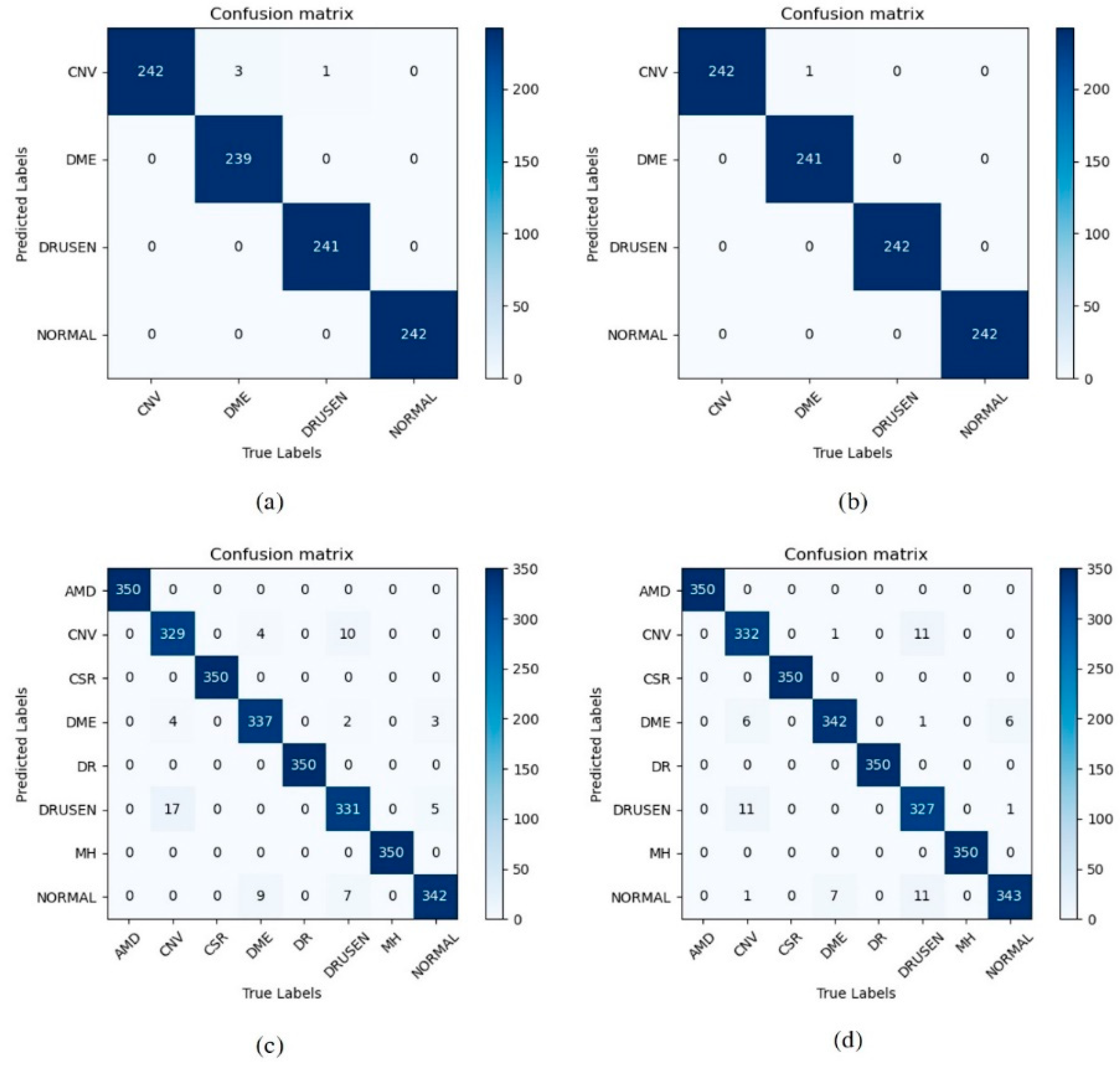
In order to visualize the performance of each model more intuitively, we use the confusion matrix to visualize the matching results between the model predictions and the true categories. The results obtained by our models on the OCT2017 and OCT-C8 datasets using different loss functions, respectively, are shown in Figure 7a,c are the results when CrossEntropy is applied, and Figure 7b,d represent the results obtained by the PolyLoss function. The diagonal elements in the confusion matrix represent the correct classification, and the remaining elements represent the misclassification.

4. Discussion

As can be seen from Table 2, EfficientNetV2 achieved an accuracy of 0.975 in the CNV category, and the highest accuracy of 0.988 was obtained in the normal category, with an F1-Score of 0.953 and 0.976 in the CNV and normal, respectively. The category accuracies of 0.986 and 0.977 were achieved in the DME and DRUSEN, respectively, while the VIT model obtained an overall lower evaluation metric than EfficientNetV2 on all four categories. Both Swin Transformer and our model achieved more than 99% accuracy on a single category, and the evaluation metrics achieved a score of 1 on the normal category. Table 3 shows that when using the PolyLoss function, EfficientNetV2 shows a slight decrease in diagnostic performance on the CNV and DRUSEN categories and a slight increase on the DME and NORMAL categories. The evaluation metrics for the three retinal disease diagnoses improved on Swin Transformer and our model. Compared to the Swin Transformer, our model obtained a higher performance evaluation with a category diagnostic accuracy of 0.999 for both CNV and DME. An accuracy score of 1 was obtained on DEUSEN and normal fundus.
Table 6 is the average of the experimental results obtained using the CrossEntropy and PolyLoss functions on the OCT2017 and OCT-C8 datasets, respectively. We observed that the performance of the EfficientNetV2 network was better than that of VIT when using CrossEntropy loss, with average accuracies of 98.2% and 96.5%, respectively. However, the Swin Transformer model achieved a 3.3% average accuracy improvement over EfficientNetV2 and performed better. We achieved an average accuracy of 99.8% using Swin Transformer V2, which improved on Precision, Recall, Specificity, and F1-Score compared to the Swin Transformer. When the loss function was changed from CrossEntropyLoss to Polyloss, although the Swin Transformer network achieved the same accuracy, it improved in several other evaluation metrics. It can be seen that when using PolyLoss, compared with CrossEntropyLoss, Swin Transformer V2 showed an improvement in Performance, with a 0.3% increase in Precision, a 0.4% increase in Recall, and a 0.1% increase in F1-Score. Swin Transformer V2 achieved 100% Precision, Recall, and Sensitivity in the DME, DRUSEN, and NORMAL categories and achieved near 1.0 accuracy in the CNV, DME, DRUSEN, and NORMAL categories. This proves the excellent classification ability of Swin Transformer V2 on the OCT dataset and that using the PolyLoss loss function can further improve the performance of the network.
On the OCT-C8 dataset, this method outperformed VIT and Swin Transformer, and using the PolyLoss loss function further improved performance, resulting in the best average performance. After using the PolyLoss loss function, Swin Transformer and our Swin Transformer V2 achieved 100% accuracy in the ADM, CSR, DR, and MH categories. In summary, in our experiments, Swin Transformer V2 demonstrated excellent classification ability on the OCT dataset. In addition, we found that using the PolyLoss loss function can further improve the performance of the network.
In addition, we compared our results with other studies. Table 7 shows the results of our comparison. Through comparison, we found that our Swin Transformer V2 improved with PolyLoss, achieving better accuracy and sensitivity performance. This demonstrates the reliability of our method in OCT image classification. These results indicate that our method has high reliability and accuracy in OCT image classification. Our Swin Transformer V2 improved with PolyLoss not only performs well in terms of accuracy, but also achieves good results in terms of sensitivity. These achievements provide strong support for our research in the field of OCT image classification and lay a solid foundation for future research.
Figure 7a,b are the confusion matrices of Swin Transformer V2 using CrossEntropyLoss and PolyLoss when tested with 968 images in the OCT2017 dataset, respectively. Figure 8b represents that the model judged a DME image as CNV disease, while it made zero errors in other categories, thus proving the excellent classification ability of the network. Figure 7c,d are the confusion matrices using two loss functions on 2800 test images in OCT-C8, respectively. As can be seen, the network has successfully classified AMD, CSR, DR, and MH data.
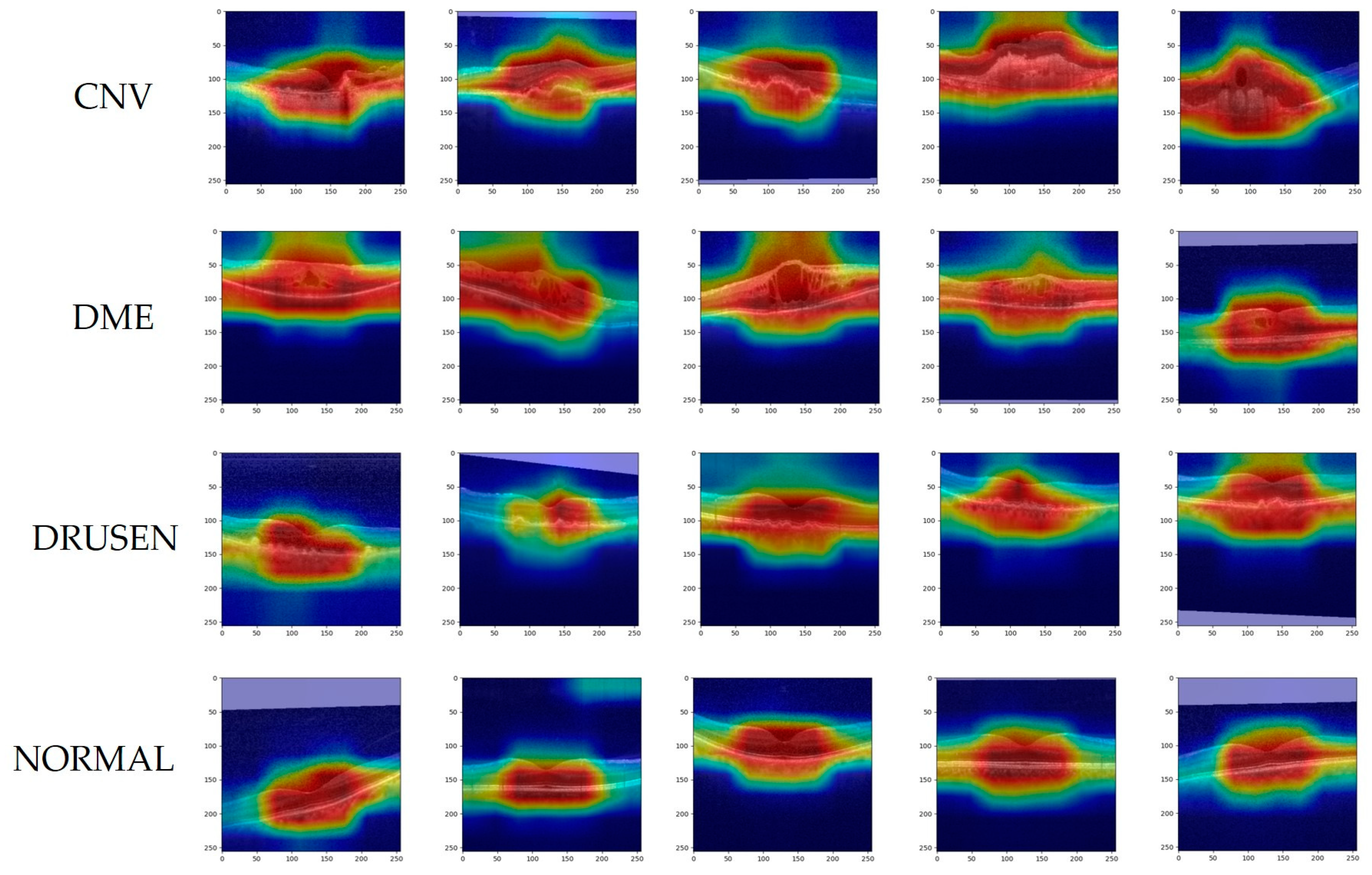
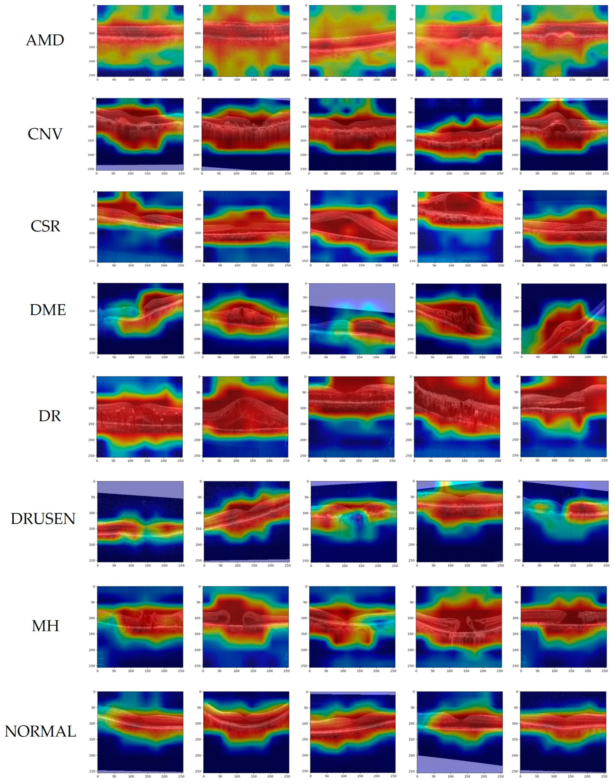
For the trained OCT model, we use Grad-CAM to visualize the decision-making mechanism of the prediction. Grad-CAM is a gradient-based deep network visualization method that explains the classification basis of deep neural network models in the form of heat maps, making category judgments through the pixels of the image. Figure 8 and Figure 9 show heatmaps of the prediction results for the OCT2017 and OCT-C8 datasets, respectively. The colors of the heatmap represent regions of interest, with red indicating high correlation with the target category and blue indicating less attention to the region. The purple area is the result of filling the blank area after data enhancement of the image. Meanwhile, lesion regions show up as a darker red color in disease OCT images. As shown in Figure 8, the second row of images shows the Grad-CAM of the DME image, and from the third image, it can be observed that the region of susceptibility contains the macular edema lesion. The image in the third row and fourth column of Figure 8 shows the region of interest for Drusen and also the region where the lesion occurred. Figure 9 is a partial image of the heat maps of the eight disease categories on the OCT-C8 dataset, showing the prediction of the heat maps of the lesion regions of each disease by our trained model. Grad-CAM helps us to see the regions of interest that the model focuses on when making a prediction, and thus to understand the decision-making process of the prediction. It is worth noting that this focus on the region of interest is also consistent with the ophthalmologist’s observation and diagnostic process.

5. Conclusions

In this paper, a multi-fundus disease classification model based on Swin Transformer V2 and the PolyLoss loss function was proposed. By comparing two different loss functions, it has been demonstrated that the PolyLoss function can enhance the model’s functionality. In the final experiment, an evaluation index close to 1 was achieved on the OCT2017 dataset, proving the good performance of the model in classifying OCT images. To validate the generalization ability of the network, it was trained and evaluated on OCT-C8, attaining a score of 1 for accuracy and other assessment metrics in half of the OCT illness categories and an average accuracy of 99.5% on the OCT-C8 dataset, proving the effectiveness of our designed model in classifying fundus diseases on OCT images.
The basic Swin Transformer V2 demonstrated strong performance on the publicly available OCT2017 dataset, making further improvements challenging. In clinical practice, misdiagnosis and missed diagnosis can lead to serious medical accidents and cause great pain to patients. The aim of our work is to improve the accuracy of model automatic diagnosis as much as possible to reduce the occurrence of misdiagnosis and missed diagnosis. However, by using polynomial loss and optimizing the network parameters, we were able to achieve a comprehensive improvement in performance metrics at a high-performance level of 99.7%, achieving a score close to 1. This indicates that our modified network model exhibits superior diagnostic capabilities. Although the magnitude of improvement is relatively small, it has positive implications for reducing misdiagnosis and improving diagnosis.
However, despite the good progress made by deep learning models in identifying abnormalities on retinal OCT images, due to the limited dataset, it is not possible to verify how well they perform on other retinal OCT data. In the future, more retinal OCT data will be sought to validate and improve the network. In addition, turning a network model into a powerful tool in the hands of clinical ophthalmologists in real life is also a major challenge, requiring more professionals to work together to turn theoretical methods into products that improve ophthalmic diagnosis.

Author Contributions

Conceptualization, Z.L., Y.H. and X.Y.; Methodology, Z.L., Y.H. and X.Y.; Data curation, Y.H.; Formal analysis, Y.H.; Writing—original draft preparation, Y.H.; Writing—review and editing, Z.L. and X.Y. All authors have read and agreed to the published version of the manuscript.

Funding

This research received no external funding.

Institutional Review Board Statement

Not applicable.

Informed Consent Statement

Informed consent was obtained from all subjects involved in the study.

Data Availability Statement

Data is contained within the article.

Conflicts of Interest

The authors declare no conflict of interest.

References

  1. Prem Senthil, M.; Khadka, J.; Gilhotra, J.S.; Simon, S.; Pesudovs, K. Exploring the quality of life issues in people with retinal diseases: A qualitative study. J. Patient-Rep. Outcomes 2017, 1, 15. [Google Scholar] [CrossRef] [PubMed]
  2. Huang, D.; Swanson, E.A.; Lin, C.P.; Schuman, J.S.; Stinson, W.G.; Chang, W.; Hee, M.R.; Flotte, T.; Gregory, K.; Puliafito, C.A. Optical coherence tomography. Science 1991, 254, 1178–1181. [Google Scholar] [CrossRef] [PubMed]
  3. Doi, K. Computer-aided diagnosis in medical imaging: Historical review, current status and future potential. Comput. Med. Imaging Graph. Off. J. Comput. Med. Imaging Soc. 2007, 31, 198–211. [Google Scholar] [CrossRef] [PubMed]
  4. LeCun, Y.; Bengio, Y.; Hinton, G. Deep learning. Nature 2015, 521, 436–444. [Google Scholar] [CrossRef]
  5. Lecun, Y.; Bottou, L.; Bengio, Y.; Haffner, P. Gradient-based learning applied to document recognition. Proc. IEEE 1998, 86, 2278–2324. [Google Scholar] [CrossRef]
  6. Krizhevsky, A.; Sutskever, I.; Hinton, G.E. ImageNet Classification with Deep Convolutional Neural Networks. Commun. ACM 2017, 60, 84–90. [Google Scholar] [CrossRef]
  7. Simonyan, K.; Zisserman, A. Very Deep Convolutional Networks for Large-Scale Image Recognition. arXiv 2015, arXiv:1409.1556. [Google Scholar]
  8. Szegedy, C.; Liu, W.; Jia, Y.Q.; Sermanet, P.; Reed, S.; Anguelov, D.; Erhan, D.; Vanhoucke, V.; Rabinovich, A. Going Deeper with Convolutions. In Proceedings of the IEEE Conference on Computer Vision and Pattern Recognition (CVPR), Boston, MA, USA, 7–12 June 2015; pp. 1–9. [Google Scholar]
  9. He, K.M.; Zhang, X.Y.; Ren, S.Q.; Sun, J. Deep Residual Learning for Image Recognition. In Proceedings of the 2016 IEEE Conference on Computer Vision and Pattern Recognition (CVPR), Seattle, WA, USA, 27–30 June 2016; pp. 770–778. [Google Scholar]
  10. Huang, G.; Liu, Z.; van der Maaten, L.; Weinberger, K.Q. Densely Connected Convolutional Networks. In Proceedings of the 30th IEEE/CVF Conference on Computer Vision and Pattern Recognition (CVPR), Honolulu, HI, USA, 21–26 July 2017; pp. 2261–2269. [Google Scholar]
  11. Howard, A.G.; Zhu, M.; Chen, B.; Kalenichenko, D.; Wang, W.; Weyand, T.; Andreetto, M.; Adam, H. MobileNets: Efficient Convolutional Neural Networks for Mobile Vision Applications. arXiv 2017, arXiv:1704.04861. [Google Scholar]
  12. Tan, M.X.; Le, Q.V. EfficientNet: Rethinking Model Scaling for Convolutional Neural Networks. In Proceedings of the 36th International Conference on Machine Learning (ICML), Long Beach, CA, USA, 9–15 June 2019. [Google Scholar]
  13. Vaswani, A.; Shazeer, N.; Parmar, N.; Uszkoreit, J.; Jones, L.; Gomez, A.N.; Kaiser, L.; Polosukhin, I. Attention Is All You Need. In Proceedings of the 31st Annual Conference on Neural Information Processing Systems (NIPS), Long Beach, CA, USA, 4–9 December 2017. [Google Scholar]
  14. Liu, Z.; Lin, Y.T.; Cao, Y.; Hu, H.; Wei, Y.X.; Zhang, Z.; Lin, S.; Guo, B.N. Swin Transformer: Hierarchical Vision Transformer using Shifted Windows. In Proceedings of the 18th IEEE/CVF International Conference on Computer Vision (ICCV), Electr Network, Montreal, BC, Canada, 11–17 October 2021; pp. 9992–10002. [Google Scholar]
  15. Dosovitskiy, A.; Beyer, L.; Kolesnikov, A.; Weissenborn, D.; Zhai, X.; Unterthiner, T.; Dehghani, M.; Minderer, M.; Heigold, G.; Gelly, S.; et al. An Image is Worth 16x16 Words: Transformers for Image Recognition at Scale. arXiv 2021, arXiv:2010.11929. [Google Scholar]
  16. Liu, Z.; Hu, H.; Lin, Y.; Yao, Z.; Xie, Z.; Wei, Y.; Ning, J.; Cao, Y.; Zhang, Z.; Dong, L.; et al. Swin Transformer V2: Scaling Up Capacity and Resolution. arXiv 2022, arXiv:2111.09883. [Google Scholar]
  17. Leng, Z.; Tan, M.; Liu, C.; Cubuk, E.D.; Shi, X.; Cheng, S.; Anguelov, D. PolyLoss: A Polynomial Expansion Perspective of Classification Loss Functions. arXiv 2022, arXiv:2204.12511. [Google Scholar]
  18. Selvaraju, R.R.; Cogswell, M.; Das, A.; Vedantam, R.; Parikh, D.; Batra, D. Grad-CAM: Visual Explanations from Deep Networks via Gradient-Based Localization. Int. J. Comput. Vis. 2020, 128, 336–359. [Google Scholar] [CrossRef]
  19. Lee, C.S.; Baughman, D.M.; Lee, A.Y. Deep learning is effective for the classification of OCT images of normal versus Age-related Macular Degeneration. Ophthalmology. Retina 2017, 1, 322–327. [Google Scholar] [CrossRef] [PubMed]
  20. Wang, D.; Wang, L. On OCT Image Classification via Deep Learning. IEEE Photonics J. 2019, 11, 1–14. [Google Scholar] [CrossRef]
  21. Islam, K.T.; Wijewickrema, S.; Leary, S.O. Identifying Diabetic Retinopathy from OCT Images using Deep Transfer Learning with Artificial Neural Networks. In Proceedings of the 2019 IEEE 32nd International Symposium on Computer-Based Medical Systems (CBMS), Cordoba, Spain, 5–7 June 2019; pp. 281–286. [Google Scholar]
  22. Rong, Y.B.; Xiang, D.H.; Zhu, W.F.; Yu, K.; Shi, F.; Fan, Z.; Chen, X.J. Surrogate-Assisted Retinal OCT Image Classification Based on Convolutional Neural Networks. IEEE J. Biomed. Health Inform. 2019, 23, 253–263. [Google Scholar] [CrossRef]
  23. Fang, L.Y.; Wang, C.; Li, S.T.; Rabbani, H.; Chen, X.D.; Liu, Z.M. Attention to Lesion: Lesion-Aware Convolutional Neural Network for Retinal Optical Coherence Tomography Image Classification. IEEE Trans. Med. Imaging 2019, 38, 1959–1970. [Google Scholar] [CrossRef]
  24. Singh, A.; Rasheed, M.A.; Zelek, J.; Lakshminarayanan, V. Interpretation of deep learning using attributions: Application to ophthalmic diagnosis. In Proceedings of the Conference on Applications of Machine Learning, Electr Network, Online, 24 August–4 September 2020. [Google Scholar]
  25. Wang, C.; Jin, Y.; Chen, X.; Liu, Z. Automatic Classification of Volumetric Optical Coherence Tomography Images via Recurrent Neural Network. Sens. Imaging 2020, 21, 32. [Google Scholar] [CrossRef]
  26. Arefin, R.; Samad, M.D.; Akyelken, F.A.; Davanian, A.; Soc, I.C. Non-transfer Deep Learning of Optical Coherence Tomography for Post-hoc Explanation of Macular Disease Classification. In Proceedings of the 9th IEEE International Conference on Healthcare Informatics (IEEE ICHI), Electr Network, Victoria, BC, Canada, 9–12 August 2021; pp. 48–52. [Google Scholar]
  27. Latha, V.; Ashok, L.R.; Sreeni, K.G.; IEEE. Automated Macular Disease Detection using Retinal Optical Coherence Tomography images by Fusion of Deep Learning Networks. In Proceedings of the 27th National Conference on Communications (NCC), Electr Network, Kanpur, India, 27–30 July 2021; pp. 333–338. [Google Scholar]
  28. Liu, X.M.; Bai, Y.J.; Cao, J.; Yao, J.P.; Zhang, Y.; Wang, M. Joint disease classification and lesion segmentation via one-stage attention-based convolutional neural network in OCT images. Biomed. Signal Process. Control 2022, 71, 103087. [Google Scholar] [CrossRef]
  29. Esfahani, E.N.; Daneshmand, P.G.; Rabbani, H.; Plonka, G. Automatic Classification of Macular Diseases from OCT Images Using CNN Guided with Edge Convolutional Layer. In Proceedings of the Annual International Conference of the IEEE Engineering in Medicine and Biology Society, Glasgow, UK, 11–15 July 2022; pp. 3858–3861. [Google Scholar] [CrossRef]
  30. He, J.Z.; Wang, J.X.; Han, Z.Y.; Ma, J.; Wang, C.J.; Qi, M. An interpretable transformer network for the retinal disease classification using optical coherence tomography. Sci. Rep. 2023, 13, 3637. [Google Scholar] [CrossRef]
  31. Ibrahim, M.R.; Fathalla, K.M.; Youssef, S.M. HyCAD-OCT: A Hybrid Computer-Aided Diagnosis of Retinopathy by Optical Coherence Tomography Integrating Machine Learning and Feature Maps Localization. Appl. Sci. 2020, 10, 4716. [Google Scholar] [CrossRef]
  32. Ai, Z.; Huang, X.; Feng, J.; Wang, H.; Tao, Y.; Zeng, F.X.; Lu, Y.P. FN-OCT: Disease Detection Algorithm for Retinal Optical Coherence Tomography Based on a Fusion Network. Front. Neuroinform. 2022, 16, 876927. [Google Scholar] [CrossRef] [PubMed]
  33. Arkin, E.; Yadikar, N.; Xu, X.B.; Aysa, A.; Ubul, K. A survey: Object detection methods from CNN to transformer. Multimed. Tools Appl. 2023, 82, 21353–21383. [Google Scholar] [CrossRef]
  34. Hendria, W.F.; Phan, Q.T.; Adzaka, F.; Jeong, C. Combining transformer and CNN for object detection in UAV imagery. ICT Express 2023, 9, 258–263. [Google Scholar] [CrossRef]
  35. Kermany, D.S.; Goldbaum, M.; Cai, W.J.; Valentim, C.C.S.; Liang, H.Y.; Baxter, S.L.; McKeown, A.; Yang, G.; Wu, X.K.; Yan, F.B.; et al. Identifying Medical Diagnoses and Treatable Diseases by Image-Based Deep Learning. Cell 2018, 172, 1122–1131.e9. [Google Scholar] [CrossRef] [PubMed]
  36. Subramanian, M.; Shanmugavadivel, K.; Naren, O.S.; Premkumar, K.; Rankish, K. Classification of Retinal OCT Images Using Deep Learning. In Proceedings of the 2022 International Conference on Computer Communication and Informatics (ICCCI), Coimbatore, India, 25–27 January 2022; pp. 1–7. [Google Scholar]
  37. Subramanian, M.; Kumar, M.S.; Sathishkumar, V.E.; Prabhu, J.; Karthick, A.; Ganesh, S.S.; Meem, M.A. Diagnosis of Retinal Diseases Based on Bayesian Optimization Deep Learning Network Using Optical Coherence Tomography Images. Comput. Intell. Neurosci. 2022, 2022, 8014979. [Google Scholar] [CrossRef] [PubMed]
  38. Tan, M.X.; Le, Q.V. EfficientNetV2: Smaller Models and Faster Training. In Proceedings of the International Conference on Machine Learning (ICML), Electr Network, Virtual Event, 18–24 July 2021; pp. 7102–7110. [Google Scholar]
  39. Szegedy, C.; Vanhoucke, V.; Ioffe, S.; Shlens, J.; Wojna, Z.; IEEE. Rethinking the Inception Architecture for Computer Vision. In Proceedings of the 2016 IEEE Conference on Computer Vision and Pattern Recognition (CVPR), Seattle, WA, USA, 27–30 June 2016; pp. 2818–2826. [Google Scholar]
  40. Sandler, M.; Howard, A.; Zhu, M.L.; Zhmoginov, A.; Chen, L.C. MobileNetV2: Inverted Residuals and Linear Bottlenecks. In Proceedings of the 31st IEEE/CVF Conference on Computer Vision and Pattern Recognition (CVPR), Salt Lake City, Salt Lake City, UT, USA, 18–23 June 2018; pp. 4510–4520. [Google Scholar]
  41. Kamran, S.A.; Tavakkoli, A.; Zuckerbrod, S.L. Improving robustness using joint attention network for detecting retinal degeneration from optical coherence tomography images. In Proceedings of the IEEE International Conference on Image Processing (ICIP), Electr Network, Abu Dhabi, United Arab Emirates, 25–28 October 2020; pp. 2476–2480. [Google Scholar]
  42. Chollet, F. Xception: Deep Learning with Depthwise Separable Convolutions. In Proceedings of the 30th IEEE/CVF Conference on Computer Vision and Pattern Recognition (CVPR), Honolulu, HI, USA, 21–26 July 2017; pp. 1800–1807. [Google Scholar]
  43. Amit Kamran, S.; Saha, S.; Shihab Sabbir, A.; Tavakkoli, A. Optic-Net: A Novel Convolutional Neural Network for Diagnosis of Retinal Diseases from Optical Tomography Images. arXiv 2019, arXiv:1910.05672. [Google Scholar]
  44. Yoo, T.K.; Choi, J.Y.; Kim, H.K. Feasibility study to improve deep learning in OCT diagnosis of rare retinal diseases with few-shot classification. Med. Biol. Eng. Comput. 2021, 59, 401–415. [Google Scholar] [CrossRef]
  45. Sathishkumar, V.E.; Park, J.; Cho, Y. Seoul bike trip duration prediction using data mining techniques. IET Intell. Transp. Syst. 2020, 14, 1465–1474. [Google Scholar] [CrossRef]
  46. Nazir, T.; Nawaz, M.; Rashid, J.; Mahum, R.; Masood, M.; Mehmood, A.; Ali, F.; Kim, J.; Kwon, H.Y.; Hussain, A. Detection of Diabetic Eye Disease from Retinal Images Using a Deep Learning based CenterNet Model. Sensors 2021, 21, 5283. [Google Scholar] [CrossRef]
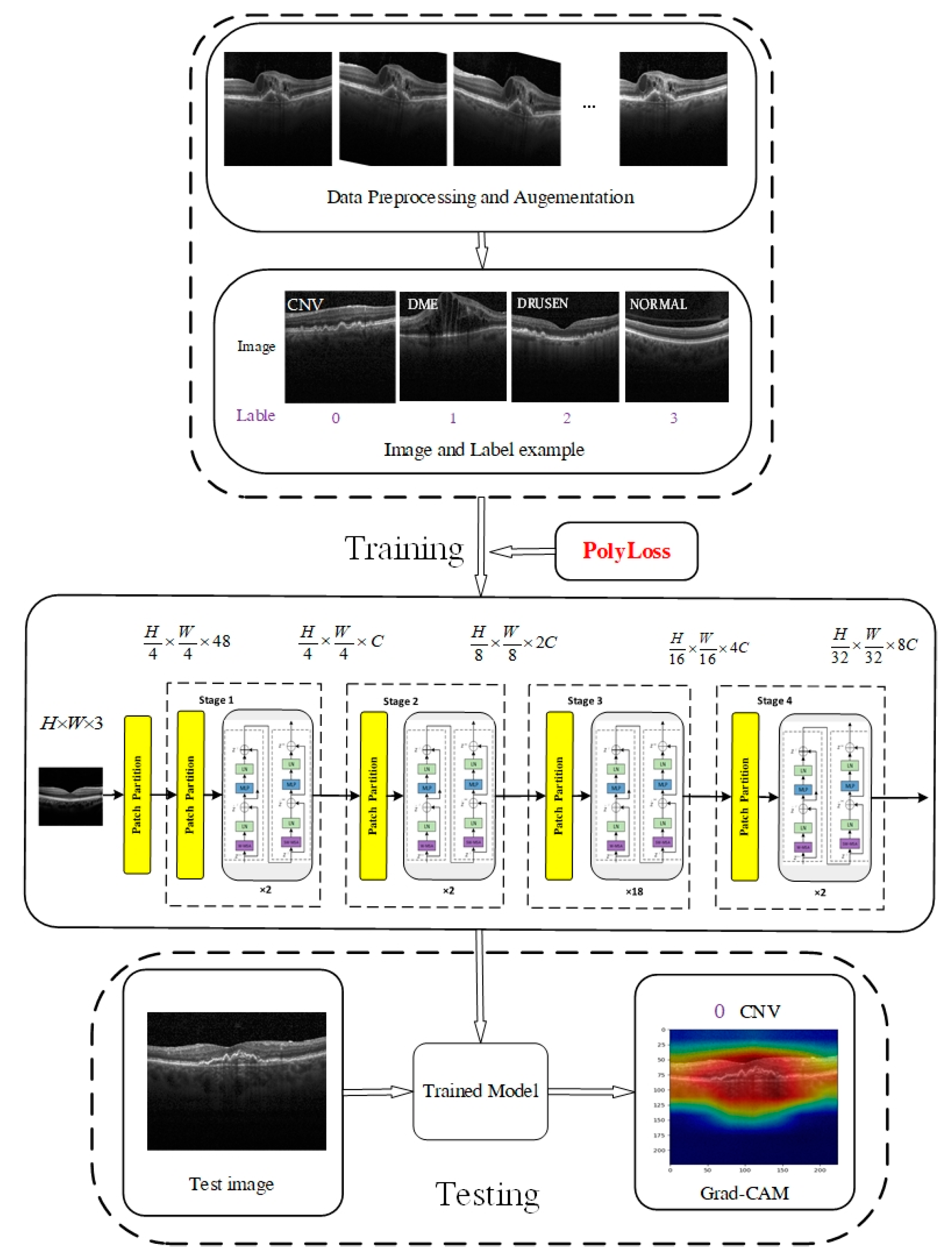
Figure 1. The overall framework of the proposed method.
Jimaging 09 00203 g001
Figure 2. (a) he overall architecture of Swin Transformer V2. (b) Two successive Swin Transformer V2 blocks.
Jimaging 09 00203 g002
Figure 3. (a) The hierarchical structure of Swin Transformer V2 for extracting multi-scale feature representation. (b) An illustration of the shifted window strategy for computing self-attention in the Swin Transformer V2 architecture.
Jimaging 09 00203 g003
Figure 4. Illustration of an efficient batch computation approach for self-attention in shifted window partitioning.
Jimaging 09 00203 g004
Figure 5. Optical coherence tomography images from the OCT2017 dataset. The panels display images of choroidal neovascularization (CNV) on the far left, diabetic macular edema (DME) on the middle left, drusen on the middle right, and a normal image on the far right.
Jimaging 09 00203 g005
Figure 6. Displays examples of the eight classes in the OCT-C8 dataset, including AMD, CNV, CSR, DME, DR, DRUSEN, MH, and NORMAL.
Jimaging 09 00203 g006
Figure 7. The Confusion matrix of our model on (a) OCT2017 (CrossEntropyLoss), (b) OCT2017 (PolyLoss), (c) OCT-C8 (CrossEntropyLoss), and (d) OCT-C8 (PolyLoss).
Jimaging 09 00203 g007
Figure 8. Gradient-weight class activation mapping on OCT2017 of our proposed networks.
Jimaging 09 00203 g008
Figure 9. Gradient-weight class activation mapping on OCT-C8 of our proposed networks.
Jimaging 09 00203 g009
Table 1. Classification and dataset setup for datasets OCT2017 and OCT-C8.
DatasetClassNumberTrainValidationTest
OCT2017CNV37,44736,2051000242
DME11,59010,3481000242
DRUSEN885876161000242
NORMAL26,55725,3151000242
OCT-C8AMD30002300350350
CNV30002300350350
CSR30002300350350
DME30002300350350
DR30002300350350
DRUSEN30002300350350
MH30002300350350
NORMAL30002300350350
Table 2. Classification results using OCT2017 with a CrossEntropy loss function. Significant values are in [bold].
DatasetMethodClassAccuracyPrecisionRecallSpecificityF1-Score
OCT2017EfficientNetV2CNV0.9750.9130.9960.9680.953
DME0.9860.9960.9460.9680.970
DRUSEN0.9771.00.9090.9990.952
NORMAL0.9880.9531.00.9830.976
VITCNV0.9500.8390.9920.9370.909
DME0.9750.9870.9130.9960.949
DRUSEN0.9510.9900.8140.9970.893
NORMAL0.9820.9341.00.9770.966
Swin TransformerCNV0.9950.9801.00.9930.990
DME0.9991.00.9961.00.998
DRUSEN0.9961.00.9831.00.991
NORMAL1.01.01.01.01.0
Swin Transformer V2CNV0.9960.9841.00.9940.992
DME0.9971.00.9881.00.994
DRUSEN0.9991.00.9961.00.998
NORMAL1.01.01.01.01.0
Table 3. Classification results using OCT2017 with a PolyLoss function. Significant values are in [bold].
DatasetMethodClassAccuracyPrecisionRecallSpecificityF1-Score
OCT2017EfficientNetV2CNV0.9710.8961.00.9610.945
DME0.9871.00.9461.00.972
DRUSEN0.9761.00.9051.00.950
NORMAL0.9920.9681.00.9800.984
VITCNV0.9520.8450.9920.9390.913
DME0.9780.9870.9260.9960.956
DRUSEN0.9500.9850.8140.9960.891
NORMAL0.9850.9421.00.9790.970
Swin TransformerCNV0.9970.9881.00.9960.994
DME0.9991.00.9961.00.998
DRUSEN0.9981.00.9921.00.996
NORMAL1.01.01.01.01.0
OursCNV0.9990.9961.00.9960.994
DME0.9991.01.01.00.998
DRUSEN1.01.01.01.00.996
NORMAL1.01.01.01.01.0
Table 4. Classification results using OCT-C8 with a CrossEntropy loss function. Significant values are in [bold].
DatasetMethodClassAccuracyPrecisionRecallSpecificityF1-Score
OCT-C8VITAMD1.01.01.01.01.0
CNV0.9650.8730.8460.9820.859
CSR0.9930.9580.9860.9940.972
DME0.9620.9010.7830.9880.838
DR0.9890.9540.9540.9930.954
DRUSEN0.9430.7750.7690.9680.772
MH0.9910.9770.9510.9970.964
NORMAL0.9590.7870.9200.9640.848
Swin TransformerAMD1.01.01.01.01.0
CNV0.9880.9540.9510.9930.952
CSR1.01.01.01.01.0
DME0.9900.9680.9570.9960.962
DR1.01.01.01.01.0
DRUSEN0.9850.9560.9370.9920.946
MH1.01.01.01.01.0
NORMAL0.9870.9450.9770.9920.961
Swin Transformer V2AMD1.01.01.01.01.0
CNV0.9880.9590.9400.9940.949
CSR1.01.01.01.01.0
DME0.9920.9740.9630.9960.968
DR1.01.01.01.01.0
DRUSEN0.9850.9380.9460.9910.942
MH1.01.01.01.01.0
NORMAL0.9910.9550.9770.9930.966
Table 5. Classification results using OCT-C8 with a PolyLoss loss function. Significant values are in [bold].
DatasetMethodClassAccuracyPrecisionRecallSpecificityF1-Score
OCT-C8VITAMD1.01.01.01.01.0
CNV0.9670.8930.8340.9860.862
CSR0.9940.9610.9910.9940.976
DME0.9620.8940.7940.9870.841
DR0.9890.9570.9570.9940.957
DRUSEN0.9430.7720.7740.9670.773
MH0.9920.9850.9540.9980.969
NORMAL0.9580.7810.9170.9630.844
Swin TransformerAMD1.01.01.01.01.0
CNV0.9880.9590.9430.9950.952
CSR1.01.01.01.01.0
DME0.9910.9740.9570.9960.965
DR1.01.01.01.01.0
DRUSEN0.9880.9540.9400.9930.947
MH1.01.01.01.01.0
NORMAL0.9900.9380.9860.9930.961
OursAMD1.01.01.01.01.0
CNV0.9890.9650.9490.9950.957
CSR1.01.01.01.01.0
DME0.9920.9630.9770.9950.970
DR1.01.01.01.01.0
DRUSEN0.9880.9650.9340.9950.949
MH1.01.01.01.01.0
NORMAL0.9910.9480.9800.9920.964
Table 6. Average of experimental results using CrossEntropy and PolyLoss functions on datasets OCT2017 and OCT-C8, respectively. Significant values are in bold.
DatasetMethodLossAccuracyPrecisionRecallSpecificityF1-Score
OCT2017EfficientNetV2CrossEntropy0.9820.9660.9630.9800.963
PolyLoss0.9810.9660.9630.9850.963
VITCrossEntropy0.9650.9380.9300.9770.917
PolyLoss0.9660.9400.9330.9780.933
Swin TransformerCrossEntropy0.9980.9950.9950.9980.995
Paper [30]PolyLoss0.9980.9970.9970.9990.997
Swin Transformer V2CrossEntropy0.9980.9960.9960.9990.996
OursPolyLoss0.9990.9991.00.9990.997
OCT-C8VITCrossEntropy0.9750.9030.9010.9860.901
PolyLoss0.9760.9050.9030.9860.903
Swin TransformerCrossEntropy0.9940.9780.9780.9970.978
Paper [30]PolyLoss0.9940.9780.9780.9970.978
Swin Transformer V2CrossEntropy0.9950.9780.9780.9970.978
OursPolyLoss0.9950.9800.9800.9970.980
Table 7. Experimental results using different models on the OCT2017 and OCT-C8 datasets, respectively. Significant values are indicated in bold.
DatasetModelAccuracySensitivity
OCT2017InceptionV3 [39]0.9340.978
MobileNet-v2 [40]0.9850.994
ResNet50-v1 [9]0.9930.993
Joint-Attention-Network ResNet-v1 [41]0.924
Xception [42]0.9970.997
OpticNet-71 [43]0.9980.998
Swin Transformer V1 [30]0.9980.998
Ours0.9990.999
OCT-C8VIT0.9750.986
GAN [44]0.939
Swin Transformer0.9940.997
Deep CNN [45]0.938
CenterNet [46]0.981
Ours0.9950.997
Disclaimer/Publisher’s Note: The statements, opinions and data contained in all publications are solely those of the individual author(s) and contributor(s) and not of MDPI and/or the editor(s). MDPI and/or the editor(s) disclaim responsibility for any injury to people or property resulting from any ideas, methods, instructions or products referred to in the content.