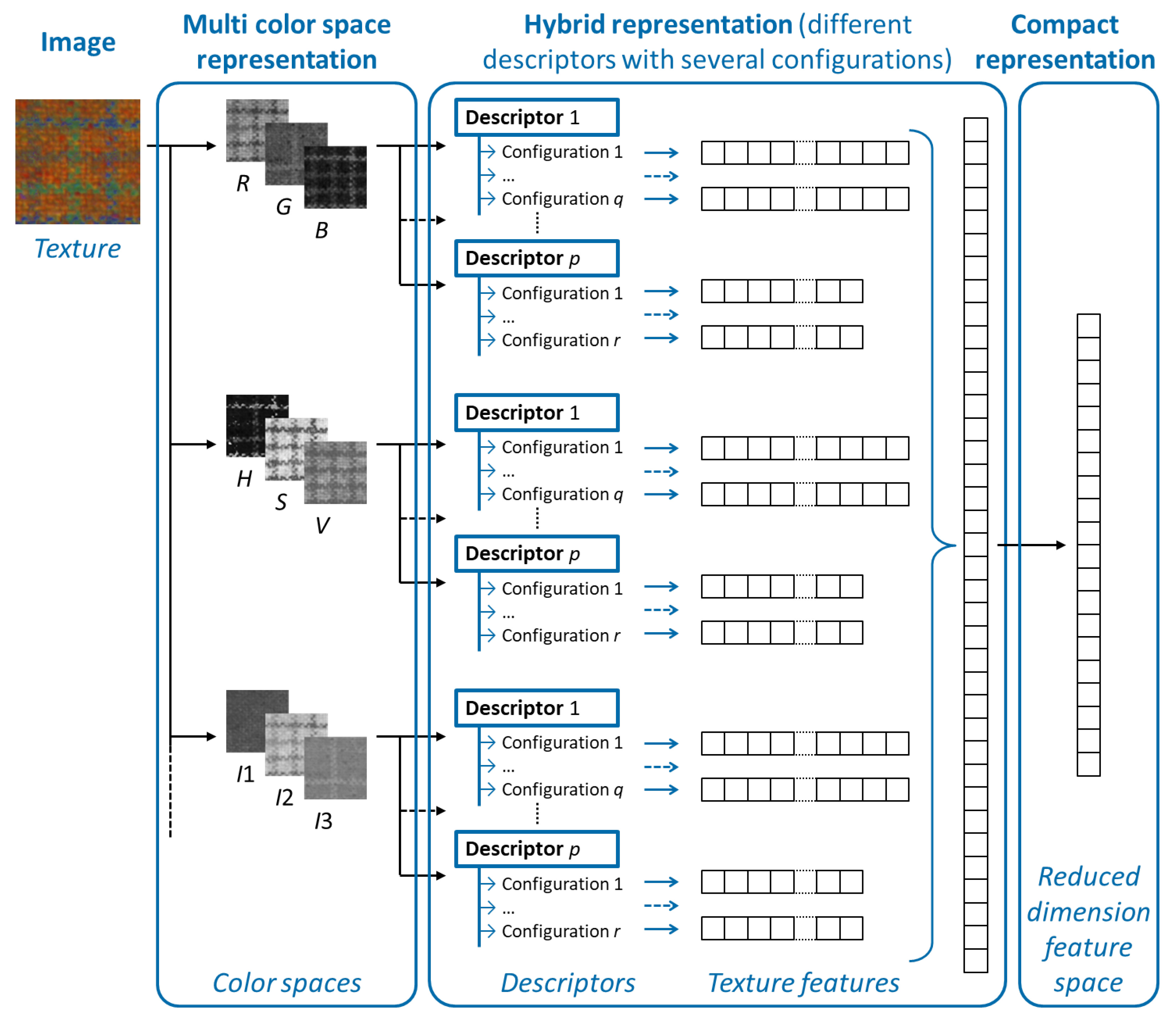
Figure 1.
The representation of a texture by the proposed compact hybrid multi-color space descriptor: the image of a color texture is firstly coded in multiple color spaces. Then, several configurations of p descriptors are used to generate a large set of color textures features. Finally, a dimensionality reduction scheme is applied to represent the color texture.
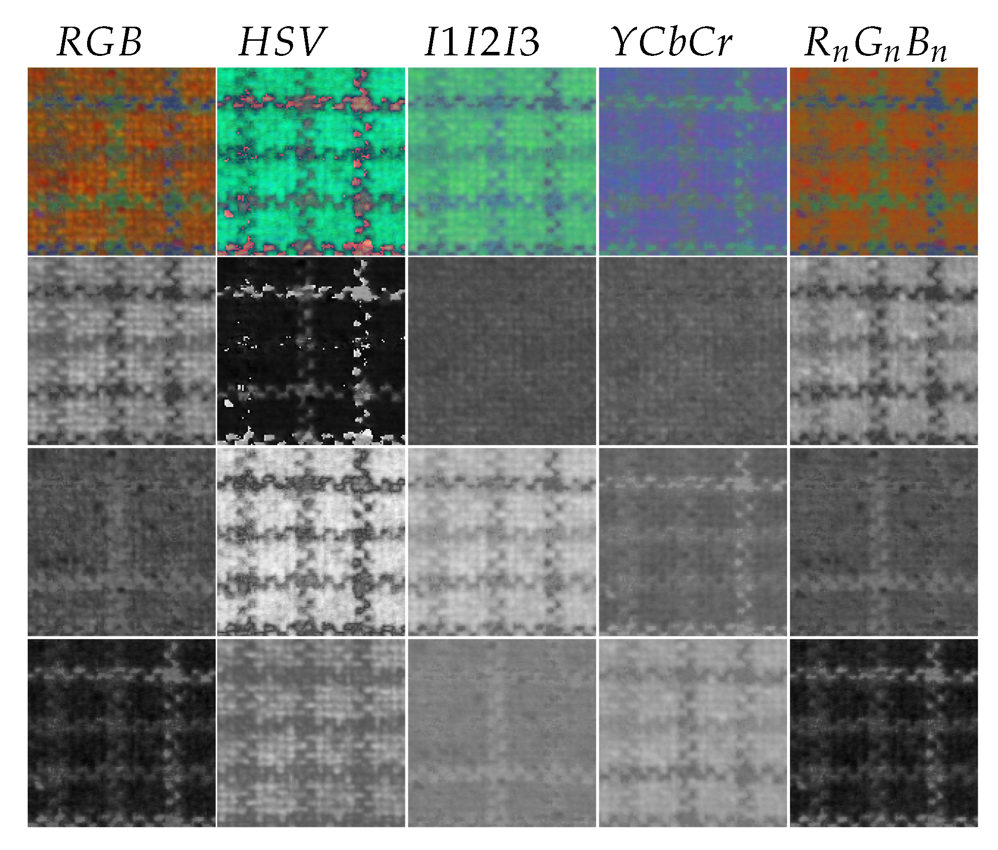
Figure 2.
Image of a texture acquired in the color space and converted into the , , and device-dependent color spaces.
Figure 2.
Image of a texture acquired in the color space and converted into the , , and device-dependent color spaces.
Figure 3.
Possible parameter settings of the RSCCM descriptor in the RGB color space: (a) 2-neighborhood and 0° direction with the component pair; (b) 2-neighborhood and direction with the component pair; (c) 2-neighborhood and direction with the component pair; (d) 2-neighborhood and direction with the component pair; and (e) 8-neighborhood with the component pair.
Figure 4.
Possible parameter settings of the EOCLBP descriptor in the color space: (a) and with the component pair; (b) and with the component pair; (c) and with the component pair; (d) and with the component pair; and (e) and with the component pair.
Figure 4.
Possible parameter settings of the EOCLBP descriptor in the color space: (a) and with the component pair; (b) and with the component pair; (c) and with the component pair; (d) and with the component pair; and (e) and with the component pair.
Figure 5.
Samples from the Outex dataset among the 68 color texture classes. Each of the 12 surface categories (from top-left to bottom-right: canvas, cardboard, carpet, foam, paper, rubber, tile, granite, sandpaper, wool, wood, and barley-rice) included in this dataset is represented herein by one image.
Figure 6.
Samples illustrating the six tree bark color textures of the NewBarkTex2 dataset (from left to right: Betula pendula, Fagus silvatica, Picea abies, Pinus silvestris, Quercus robus, and Robinia pseudacacia).
Figure 6.
Samples illustrating the six tree bark color textures of the NewBarkTex2 dataset (from left to right: Betula pendula, Fagus silvatica, Picea abies, Pinus silvestris, Quercus robus, and Robinia pseudacacia).
Figure 7.
Samples of different categories from the USPtex dataset among the 191 color texture classes.
Figure 7.
Samples of different categories from the USPtex dataset among the 191 color texture classes.
Figure 8.
Samples of different categories from the Stex dataset among the 476 color texture classes.
Figure 8.
Samples of different categories from the Stex dataset among the 476 color texture classes.
Figure 9.
Samples of the OAK wood category from the Parquet dataset among the 38 color texture classes.
Figure 9.
Samples of the OAK wood category from the Parquet dataset among the 38 color texture classes.
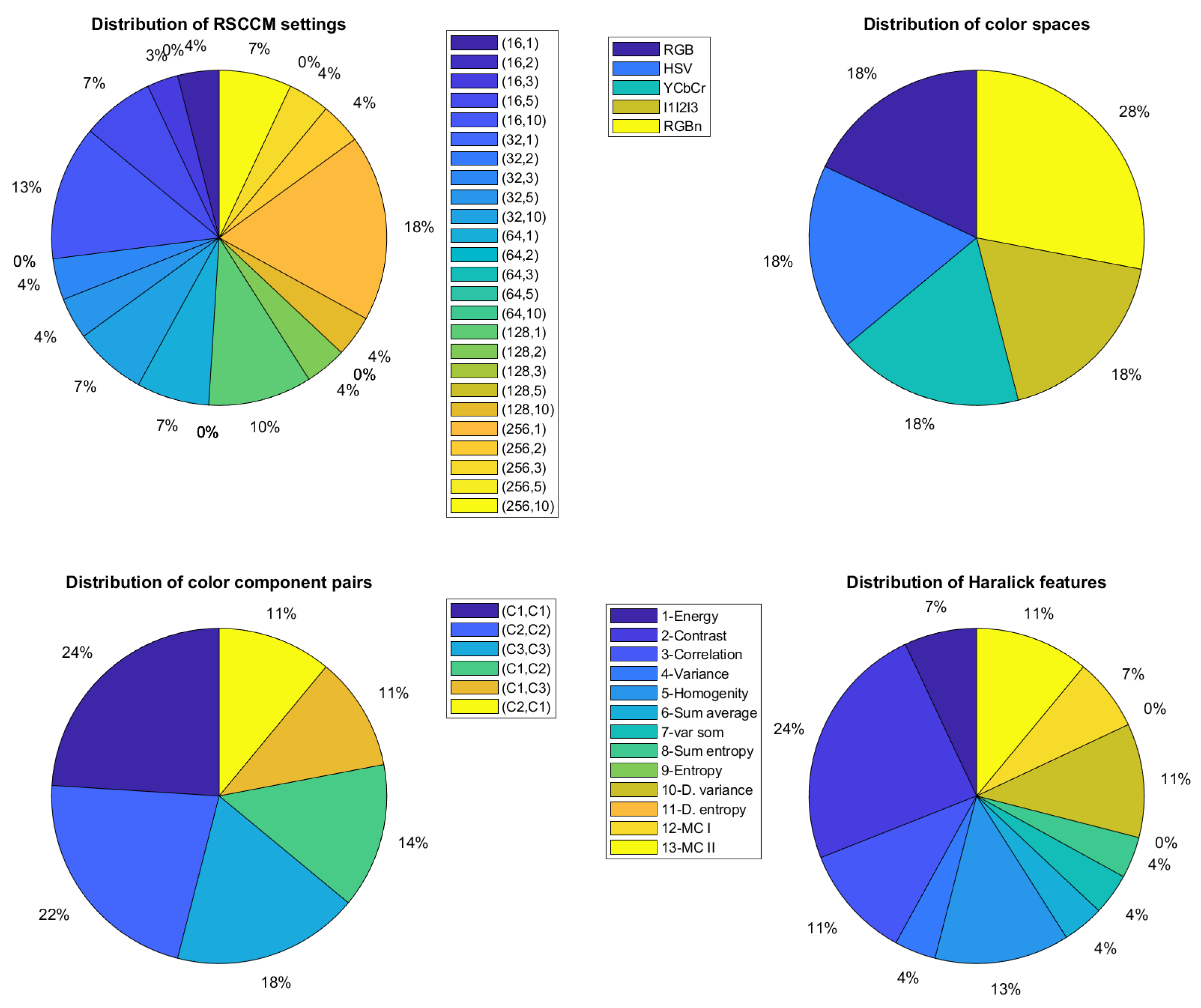
Figure 10.
Distribution of the selected features for the RSCCM descriptor with the MPMC representation for the USPtex dataset. This distribution is shown for the descriptor settings, color spaces, color component pairs and Haralick features.
Figure 10.
Distribution of the selected features for the RSCCM descriptor with the MPMC representation for the USPtex dataset. This distribution is shown for the descriptor settings, color spaces, color component pairs and Haralick features.
Figure 11.
Distribution of the selected features for the EOCLBP descriptor with the MPMC representation for the USPtex dataset. This distribution is shown for the descriptor settings, color spaces, color component pairs and statistical features.
Figure 11.
Distribution of the selected features for the EOCLBP descriptor with the MPMC representation for the USPtex dataset. This distribution is shown for the descriptor settings, color spaces, color component pairs and statistical features.
Figure 12.
Distribution of the two descriptors and the five color spaces with the CHMCS representation for the USPtex dataset.
Figure 12.
Distribution of the two descriptors and the five color spaces with the CHMCS representation for the USPtex dataset.
Table 1.
Dimensionality of color texture feature spaces.
Table 1.
Dimensionality of color texture feature spaces.
| Descriptor | | | | | Dimensionality |
|---|
| | | | | | |
| RSCCM | 1 | 1 | | 13 | 78 |
| EOCLBP | 2 | 1 | | 17 | 153 |
| RSCCM | 1 | 5 | | 13 | 390 |
| EOCLBP | 2 | 5 | | 17 | 765 |
| RSCCM | 1 | 1 | | 13 | 1950 |
| EOCLBP | 2 | 1 | | 17 | 1989 |
| RSCCM | 1 | 5 | | 13 | 9750 |
| EOCLBP | 2 | 5 | | 17 | 9945 |
Table 2.
Experimented color texture datasets.
Table 2.
Experimented color texture datasets.
| Dataset | Image | Number of | Number of | Number of |
|---|
| | Size | Classes | Images | Images/Class |
|---|
| Outex | | 68 | 1360 | 20 |
| NewBarkTex2 | | 6 | 408 | 68 |
| USPtex | | 191 | 2292 | 12 |
| Stex | | 476 | 7616 | 16 |
| Parquet | to | 38 | 228 | 6 |
| | | | | |
Table 3.
Color texture representations where is the number of considered color spaces, is the number of color component pairs considered in each color space, is the number of parameter combinations, is the number of color texture features extracted from each configuration of the descriptor, and D is the total number of color texture features.
| Representation | Descriptor | p | | | | | D |
|---|
| SPSC | RSCCM | 1 | 1 | 6 | 1 | 13 | 78 |
| SPSC | EOCLBP | 2 | 1 | 9 | 1 | 17 | 153 |
| SPMC | RSCCM | 1 | 5 | 6 | 1 | 13 | 390 |
| SPMC | EOCLBP | 2 | 5 | 9 | 1 | 17 | 765 |
| MPSC | RSCCM | 1 | 1 | 6 | 25 | 13 | 1950 |
| MPSC | EOCLBP | 2 | 1 | 9 | 13 | 17 | 1989 |
| MPMC | RSCCM | 1 | 5 | 6 | 25 | 13 | 9750 |
| MPMC | EOCLBP | 2 | 5 | 9 | 13 | 17 | 9945 |
| CHMCS | RSCCM + EOCLBP | – | 5 | – | – | – | |
Table 4.
Classification accuracy (in % of well-classified test images) for the USPtex dataset. For each descriptor, the best result reached by an SPSC representation is written in bold and underlined. The results obtained with MPMC and CHMCS representations are boxed (and bold written for CHMCS). Other italic and/or underlined annotations refer to other discussed results.
| Descriptor | Setting | | | | | | Min–Max | Mean | SPMC |
|---|
| RSCCM | (16,1) | | | | | | [68.76–91.27] | | |
| (16,2) | | | | | | [69.46–88.39] | | |
| (16,3) | | | | | | [66.41–89.44] | | |
| (16,5) | | | | | | [61.52–87.44] | | |
| (16,10) | | | | | | [58.55–82.98] | | |
| (32,1) | | | | | | [78.45–91.89] | | |
| (32,2) | | | | | | [75.65–90.40] | | |
| (32,3) | | | | | | [73.56–89.44] | | |
| (32,5) | | | | | | [71.38–87.87] | | |
| (32,10) | | | | | | [67.19–84.64] | | |
| (64,1) | | | | | | [82.37–93.11] | | |
| (64,2) | | | | | | [80.72–92.67] | | |
| (64,3) | | | | | | [77.92–91.27] | | |
| (64,5) | | | | | | [77.05–87.78] | | |
| (64,10) | | | | | | [72.51–84.56] | | |
| (128,1) | | | | | | [82.81–93.63] | | |
| (128,2) | | | | | | [80.98–92.76] | | |
| (128,3) | | | | | | [78.36–91.54] | | |
| (128,5) | | | | | | [74.87–88.83] | | |
| (128,10) | | | | | | [70.33–86.48] | | |
| (256,1) | | | | | | [83.33–94.24] | | |
| (256,2) | | | | | | [82.81–93.28] | | |
| (256,3) | | | | | | [82.46–92.41] | | |
| (256,5) | | | | | | [79.06–89.79] | | |
| (256,10) | | | | | | [74.08–86.39] | | |
| Min–Max | [71.99–83.51] | [82.98–91.89] | [76.00–94.24] | [77.75–93.37] | [58.55–85.17] | [58.55–94.24 ] | [73.46–89.60] | [88.22–95.29] |
| Mean | | | | | | [75.12–88.60] | | |
| MPSC | | | | | | [84.21–93.54] | | 95.63(84) |
| EOCLBP | (8,1) | | | | | | [80.19–89.79] | | |
| (8,2) | | | | | | [82.37–90.05] | | |
| (8,3) | | | | | | [83.71–91.10] | | |
| (8,5) | | | | | | [77.57–84.53] | | |
| (8,10) | | | | | | [60.30–73.56] | | |
| (12,2) | | | | | | | | |
| (12,3) | | | | | | [84.73–90.84] | | |
| (12,5) | | | | | | [82.72–88.37] | | |
| (12,10) | | | | | | [65.10–76.06] | | |
| (16,2) | | | | | | [83.45–91.80] | | |
| (16,3) | | | | | | [84.50–92.06] | | |
| (16,5) | | | | | | [82.37–89.79] | | |
| (16,10) | | | | | | [68.76–79.67] | | |
| Min–Max | [60.30–87.00] | [71.64–89.35] | [72.51–92.06] | [73.33–92.32] | [70.94–84.99] | [60.30–92.32] | [69.95–88.82] | [86.13–96.86] |
| Mean | | | | | | [79.18–86.44] | | |
| MPSC | | | | | | [87.00–94.59] | | 95.64(89) |
| Hybrid | Min–Max | [60.30–87.00] | [71.64–91.89] | [72.51–94.24] | [73.33–93.37] | [58.55–85.17] | [58.55–94.24] | [69.95–89.60] | [86.13–96.86] |
| Mean | | | | | | [77.90–87.50] | | |
| Hybrid | | | | | | [87.69–96.68] | | 97.70(51) |
Table 5.
Accuracy (in % of well-classified test images) obtained by the best configuration of each descriptor.
Table 5.
Accuracy (in % of well-classified test images) obtained by the best configuration of each descriptor.
| Dataset | RSCCM | EOCLBP |
|---|
| | Best Result | Setting | Color Space | Best Result | Setting | Color Space |
|---|
| Outex | | | | | | |
| NewBarkTex2 | | | | | | |
| USPtex | | | | | | |
| Stex | | | | | | |
| Parquet | | | | | | |
Table 6.
Distribution of the selected features.
Table 6.
Distribution of the selected features.
| Dataset | | Descriptor | Color Spaces |
|---|
| | | RSCCM (25, 6) | EOCLBP (13, 9) | | | | | |
|---|
| Outex | 36 | 17 | (9, 6) | 19 | (9, 8) | 12 | 8 | 6 | 5 | 5 |
| NewBarkTex2 | 20 | 7 | (6, 5) | 13 | (8, 7) | 3 | 3 | 2 | 6 | 6 |
| USPtex | 51 | 28 | (15, 6) | 23 | (11, 9) | 19 | 5 | 5 | 13 | 9 |
| Stex | 75 | 37 | (18, 6) | 38 | (10, 6) | 19 | 20 | 16 | 9 | 11 |
| Parquet | 41 | 29 | (12, 6) | 12 | (8, 9) | 12 | 5 | 10 | 5 | 9 |
Table 7.
Accuracy obtained (in % of well-classified test images) with the CHMCS descriptor compared to other approaches. For each dataset, the highest accuracy is written in bold. The highest accuracy reached by the other approaches is underlined. “With” and “Without” refer to the selection procedure.
| Dataset | RSCCM | EOCLBP | CHMCS |
|---|
| | SPSC | SPMC | MPSC | MPMC | SPSC | SPMC | MPSC | MPMC | Without | With |
|---|
| Outex | | | | | | | | | | |
| NewBarkTex2 | | | | | | | | | | |
| USPtex | | | | | | | | | | |
| Stex | | | | | | | | | | |
| Parquet | | | | | | | | | | |
Table 8.
Dimensionality of the feature space obtained with the CHMCS descriptor compared to other approaches for each dataset.
Table 8.
Dimensionality of the feature space obtained with the CHMCS descriptor compared to other approaches for each dataset.
| Dataset | RSCCM | EOCLBP | CHMCS |
|---|
| | SPSC | SPMC | MPSC | MPMC | SPSC | SPMC | MPSC | MPMC | |
|---|
| Outex | | | | 27 | | | | 59 | 36 |
| NewBarkTex2 | | | | 24 | | | | 27 | 20 |
| USPtex | | | | 84 | | | | 89 | 51 |
| Stex | | | | 83 | | | | 67 | 75 |
| Parquet | | | | 15 | | | | 8 | 41 |
Table 9.
Comparison with handcrafted descriptors and deep learning approaches. Mean classification rates are provided (written in italic) for each approach across the five datasets. For each dataset, the best results are written in bold.
Table 9.
Comparison with handcrafted descriptors and deep learning approaches. Mean classification rates are provided (written in italic) for each approach across the five datasets. For each dataset, the best results are written in bold.
| Descriptor | Dataset | Average |
|---|
| Outex | NewBarkTex2 | USPtex | Stex | Parquet |
|---|
| Our approach |
| CHMCS | | | | | | |
| Fine-tuned CNN models |
| ResNet50 | | | | | | |
| Resnet18 | | | | | | |
| GoogleNet | | | | | | |
| AlexNet | | | | | | |
| Pretrained generic CNN models |
| ResNet-50 | | | | | | |
| ResNet-101 | | | | | | |
| ResNet-152 | | | | | | |
| VGG-VD-16 | | | | | | |
| VGG-VD-19 | | | | | | |
| Traditional handcrafted color texture descriptors |
| IOCLBP | | | | | | |
| OCLBP | | | | | | |
| LCVBP | | | | | | |
| SWOBP | | | | | | |
| Best RSCCM | | | | | | |
| Best EOCLBP | | | | | | |


 ,
, 


