
Time Is Money: Considerations for Measuring the Radiological Reading Time


Abstract
:1. Introduction
2. Materials and Methods
2.1. Data
2.2. Definitions
2.3. Simulation for Outlier Detection
2.4. Real Reporting Time
2.5. Statistics
3. Results
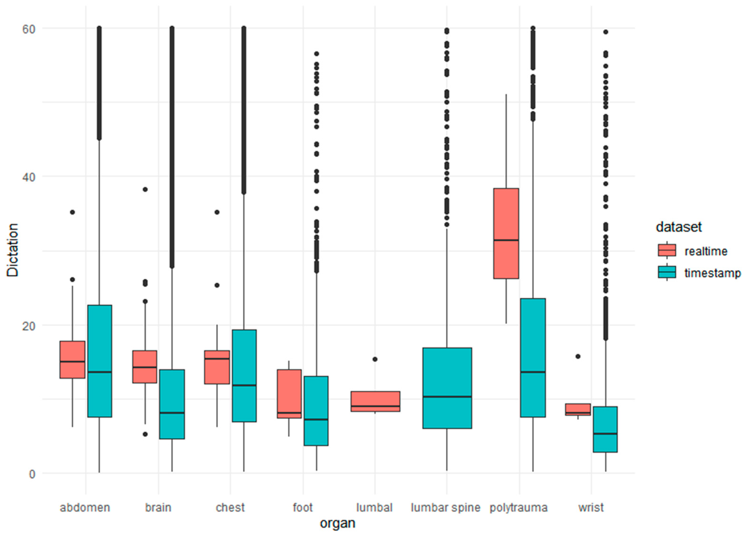
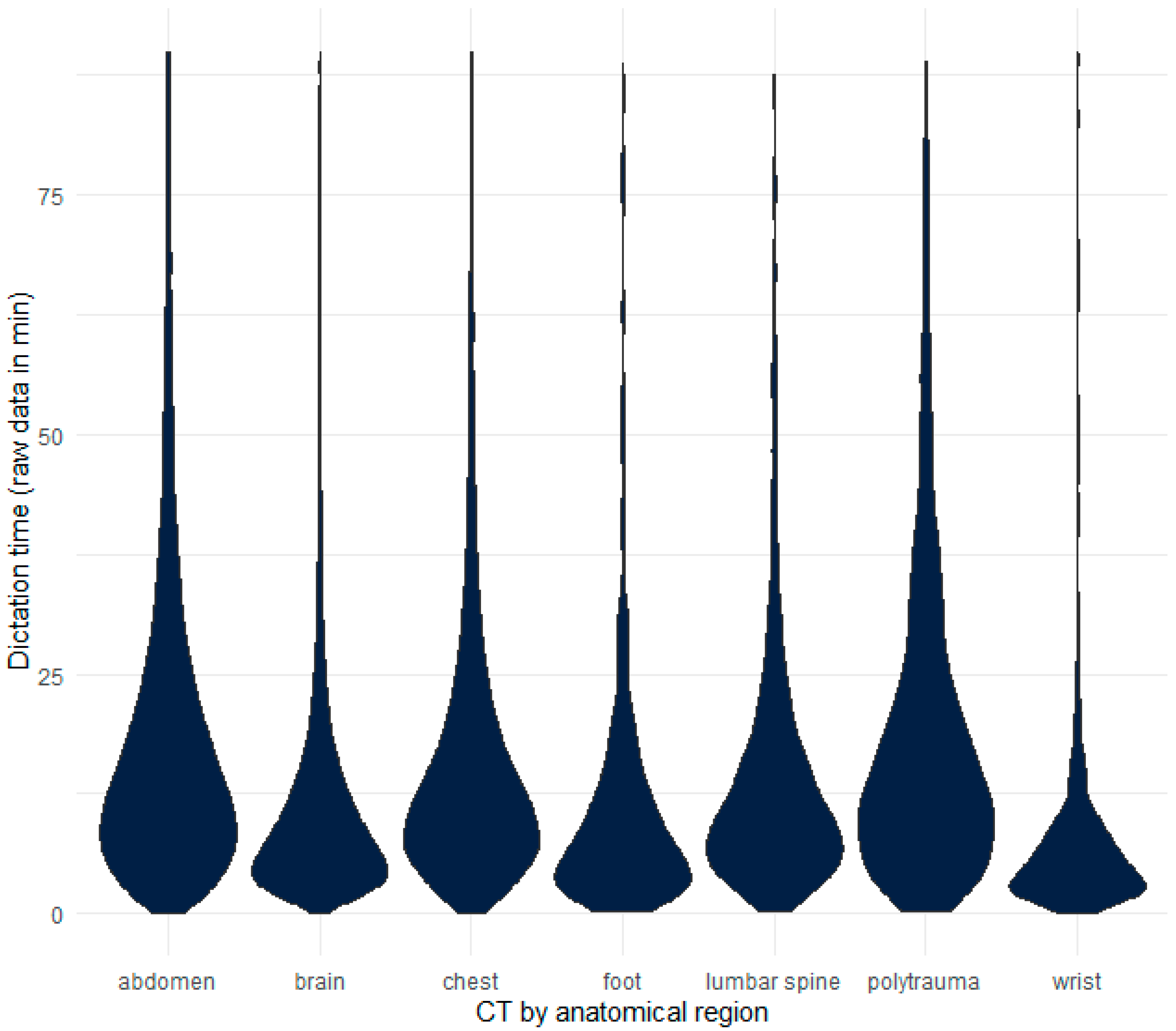
3.1. Reporting Time
Real Reporting Time
4. Discussion
5. Conclusions
Author Contributions
Funding
Institutional Review Board Statement
Informed Consent Statement
Data Availability Statement
Acknowledgments
Conflicts of Interest
Appendix A
		 #data= your timestamps
		 N<-length(data)
		 t_max<-max(data)
		 ## function,to optimize:
		 optL <- function(l.vec, m, s)
		  {
		   error <- rep(NA, length(l.vec))
		   for(i in c(1:length(l.vec)))
		     {
		     sim.df <- data.frame(x1 = rnorm(N,mean=m, sd=s), x2 = rexp(N, l.vec[i]))
		     sim <- apply(sim.df, 1, min)
		     # plot(density(sim))
		     error[i] <- sum((sort(data) - sort(sim))^2)
		     }
		   return(l.vec[which.min(error)])
		   print(l.vec)
		  }

		 ## function to optimize m
		 optM <- function(m.vec,l,s)
		  {
		   error <- rep(NA,length(m.vec))
		   for(i in c(1:length(m.vec)))
		     {
		     sim.df <- data.frame(x1=rnorm(N,m.vec[i]),sd=s, x2 = rexp(N, l))
		     sim <- apply(sim.df,1,min)
		     error[i] <- sum((sort(data)- sort(sim))^2)
		     }
		   return(m.vec[which.min(error)])
		   print(m.vec)
		  }
		 ## function to optimize SD
		 optS <- function(m,l,s.vec)
		  {
		   error <- rep(NA,length(s.vec))
		   for(i in c(1:length(s.vec)))
		     {
		     sim.df <- data.frame(x1=rnorm(N,m,sd=s.vec[i]), x2= rexp(N,l))
		     sim <- apply(sim.df,1,min)
		     error [i] <- sum((sort(data)-sort(sim))^2)
		     }
		   return(s.vec[which.min(error)])
		   print(s.vec)
		  }

		 ## Define range for search vector for l,m,s:
		 my.vec <- function(x,i){
		  x.min <- x-(x/(i^2))
		  x.max <- x+(x/(i^2))
		  my.vec <-seq(from = x.min, to = x.max, length.out = 100)
		  return(my.vec)
		 }
		 ### prepare iteration
		 ## set variables: m,s,l, i=iteration step
		 m<-30
		 s<-10
		 l<-0.03
		 #set.seed= reproducibility
		 set.seed(50)
		 ###iteration start:
		 for(i in c(1:1500)){
		  ## optimize l with m, s
		 my.l <- my.vec(l, i)
		 my.l <- my.l[my.l >0 and my.l < 1]
		 l <- optL(my.l,m, s)
		 ## optimize m with l, s
		 my.m <- my.vec(m, i)
		 my.m <- my.m[my.m >0 and my.m < 120]
		 m <- optM(my.m,l = l, s = s)
		 ## optimize s with l,m
		 my.s <- my.vec(s, i)
		 my.s <- my.s[my.s >0 and my.s < 120]
		 s <- optS(my.s,l = l, m = m)
		 ## plot each 100 iteration
		 if(i %% 100 == 0){
		  sim.df <- data.frame(x1=rnorm(N,m,sd=s), x2= rexp(N,l))
		  sim <- apply(sim.df,1,min)
		  norm <- sum(sim.df[, 1] == sim)
		  error <- sum((sort(sim) - sort(data))^2)
		  mypath<-file.path("D:/expo/PETCT/",paste("histogram_iteration_",i,".jpg",sep=""))
		  jpeg(file=mypath)
		  hist(sim,
		     main = paste("Iteration", i,"von N(my,s):", norm,", m =", sprintf("%.2f", m), ", s =", sprintf("%.2f", s), ", l =", sprintf("%.2f",l), "error = ", error),
		     xlim = c(0,t_max/3), ylim = c(0,t_max/3),
		     col = "blue",
		     breaks=300,xlab="time(min)",ylab="frequency")
		  par(new = TRUE)
		  hist(data,
		     main = "",
		     xlim = c(0,t_max/3), ylim = c(0, t_max/3),
		     breaks = 300,xlab="",ylab="")
		  dev.off()
		  }
		 }
		 write.table(
		  paste("medium:",m,
		    "n(total):",N,
		    "n(norm):",norm,
		    "standard deviation:",s,
		    "lambda exponential:",l,
		    "iteration:",i),"D:/expo/PETCT/results/information.txt",sep="\t")
		 library(truncnorm)
		 x <- rtruncnorm(n = 118, a = 0, b = Inf, mean = m, sd = s)
		 y<-summary(sim.df)
References
- Brook, R.H.; McGlynn, E.A.; Cleary, P.D. Measuring Quality of Care. N. Engl. J. Med. 1996, 335, 966–970. [Google Scholar] [CrossRef] [PubMed]
- Porter, M.E. What Is Value in Health Care? N. Engl. J. Med. 2010, 363, 2477–2481. [Google Scholar] [CrossRef] [PubMed]
- Varoquaux, G.; Cheplygina, V. Machine Learning for Medical Imaging: Methodological Failures and Recommendations for the Future. NPJ Digit. Med. 2022, 5, 1–8. [Google Scholar] [CrossRef]
- Sabol, P.; Sinčák, P.; Hartono, P.; Kočan, P.; Benetinová, Z.; Blichárová, A.; Verbóová, Ľ.; Štammová, E.; Sabolová-Fabianová, A.; Jašková, A. Explainable Classifier for Improving the Accountability in Decision-Making for Colorectal Cancer Diagnosis from Histopathological Images. J. Biomed. Inform. 2020, 109, 103523. [Google Scholar] [CrossRef] [PubMed]
- Rundo, L.; Pirrone, R.; Vitabile, S.; Sala, E.; Gambino, O. Recent Advances of HCI in Decision-Making Tasks for Optimized Clinical Workflows and Precision Medicine. J. Biomed. Inform. 2020, 108, 103479. [Google Scholar] [CrossRef] [PubMed]
- Becker, C.D.; Kotter, E.; Fournier, L.; Martí-Bonmatí, L. European Society of Radiology (ESR) Current Practical Experience with Artificial Intelligence in Clinical Radiology: A Survey of the European Society of Radiology. Insights Imaging 2022, 13, 107. [Google Scholar] [CrossRef]
- Donabedian, A. The Quality of Care: How Can It Be Assessed? JAMA 1988, 260, 1743–1748. [Google Scholar] [CrossRef] [PubMed]
- VanLare, J.M.; Conway, P.H. Value-Based Purchasing—National Programs to Move from Volume to Value. N. Engl. J. Med. 2012, 367, 292–295. [Google Scholar] [CrossRef] [PubMed] [Green Version]
- Cowan, I.A.; MacDonald, S.L.; Floyd, R.A. Measuring and Managing Radiologist Workload: Measuring Radiologist Reporting Times Using Data from a Radiology Information System: Measuring Radiologist Reporting Times. J. Med. Imaging Radiat. Oncol. 2013, 57, 558–566. [Google Scholar] [CrossRef] [PubMed]
- Eng, J. Sample Size Estimation: How Many Individuals Should Be Studied? Radiology 2003, 227, 309–313. [Google Scholar] [CrossRef] [PubMed] [Green Version]
- Zabel, A.O.J.; Leschka, S.; Wildermuth, S.; Hodler, J.; Dietrich, T.J. Subspecialized Radiological Reporting Reduces Radiology Report Turnaround Time. Insights Imaging 2020, 11, 114. [Google Scholar] [CrossRef] [PubMed]
- MacDonald, S.L.; Cowan, I.A.; Floyd, R.A.; Graham, R. Measuring and Managing Radiologist Workload: A Method for Quantifying Radiologist Activities and Calculating the Full-Time Equivalents Required to Operate a Service. J. Med. Imaging Radiat. Oncol. 2013, 57, 551–557. [Google Scholar] [CrossRef] [PubMed]
- Krupinski, E.A.; Hall, E.T.; Jaw, S.; Reiner, B.; Siegel, E. Influence of Radiology Report Format on Reading Time and Comprehension. J. Digit. Imaging 2012, 25, 63–69. [Google Scholar] [CrossRef] [PubMed] [Green Version]
- van Assen, M.; Muscogiuri, G.; Caruso, D.; Lee, S.J.; Laghi, A.; De Cecco, C.N. Artificial Intelligence in Cardiac Radiology. Radiol. Med. 2020, 125, 1186–1199. [Google Scholar] [CrossRef] [PubMed]
- Stec, N.; Arje, D.; Moody, A.R.; Krupinski, E.A.; Tyrrell, P.N. A Systematic Review of Fatigue in Radiology: Is It a Problem? Am. J. Roentgenol. 2018, 210, 799–806. [Google Scholar] [CrossRef] [PubMed]
- Sexauer, R.; Stieltjes, B.; Bremerich, J.; D’Antonoli, T.A.; Schmidt, N. Considerations on Baseline Generation for Imaging AI Studies Illustrated on the CT-Based Prediction of Empyema and Outcome Assessment. J. Imaging 2022, 8, 50. [Google Scholar] [CrossRef] [PubMed]
- Wilder-Smith, A.J.; Yang, S.; Weikert, T.; Bremerich, J.; Haaf, P.; Segeroth, M.; Ebert, L.C.; Sauter, A.; Sexauer, R. Automated Detection, Segmentation, and Classification of Pericardial Effusions on Chest CT Using a Deep Convolutional Neural Network. Diagnostics 2022, 12, 1045. [Google Scholar] [CrossRef] [PubMed]


| n (Total) | n (Norm) | Mean | Standard Deviation | Median | |
|---|---|---|---|---|---|
| Head | 45,596 | 44,743 | 16.05 | 31.27 | 16.37 |
| Chest | 33,381 | 32,797 | 15.84 | 30.21 | 16.16 |
| Abdomen | 23,483 | 22,805 | 17.92 | 31.95 | 17.75 |
| Foot | 958 | 937 | 10.96 | 20.16 | 10.80 |
| Lumbar spine | 892 | 881 | 9.14 | 13.27 | 8.91 |
| Wrist | 1322 | 1201 | 8.83 | 12.83 | 8.44 |
| Polytrauma | 2242 | 2127 | 39.2 | 52.41 | 39.36 |
| All | 107,874 | 105,491 | 16.62 | 33.11 | 16.58 |
Publisher’s Note: MDPI stays neutral with regard to jurisdictional claims in published maps and institutional affiliations. |
© 2022 by the authors. Licensee MDPI, Basel, Switzerland. This article is an open access article distributed under the terms and conditions of the Creative Commons Attribution (CC BY) license (https://creativecommons.org/licenses/by/4.0/).
Share and Cite
Sexauer, R.; Bestler, C. Time Is Money: Considerations for Measuring the Radiological Reading Time. J. Imaging 2022, 8, 208. https://doi.org/10.3390/jimaging8080208
Sexauer R, Bestler C. Time Is Money: Considerations for Measuring the Radiological Reading Time. Journal of Imaging. 2022; 8(8):208. https://doi.org/10.3390/jimaging8080208
Chicago/Turabian StyleSexauer, Raphael, and Caroline Bestler. 2022. "Time Is Money: Considerations for Measuring the Radiological Reading Time" Journal of Imaging 8, no. 8: 208. https://doi.org/10.3390/jimaging8080208
APA StyleSexauer, R., & Bestler, C. (2022). Time Is Money: Considerations for Measuring the Radiological Reading Time. Journal of Imaging, 8(8), 208. https://doi.org/10.3390/jimaging8080208