
Detecting Cocircular Subsets of a Spherical Set of Points


Abstract
:1. Introduction
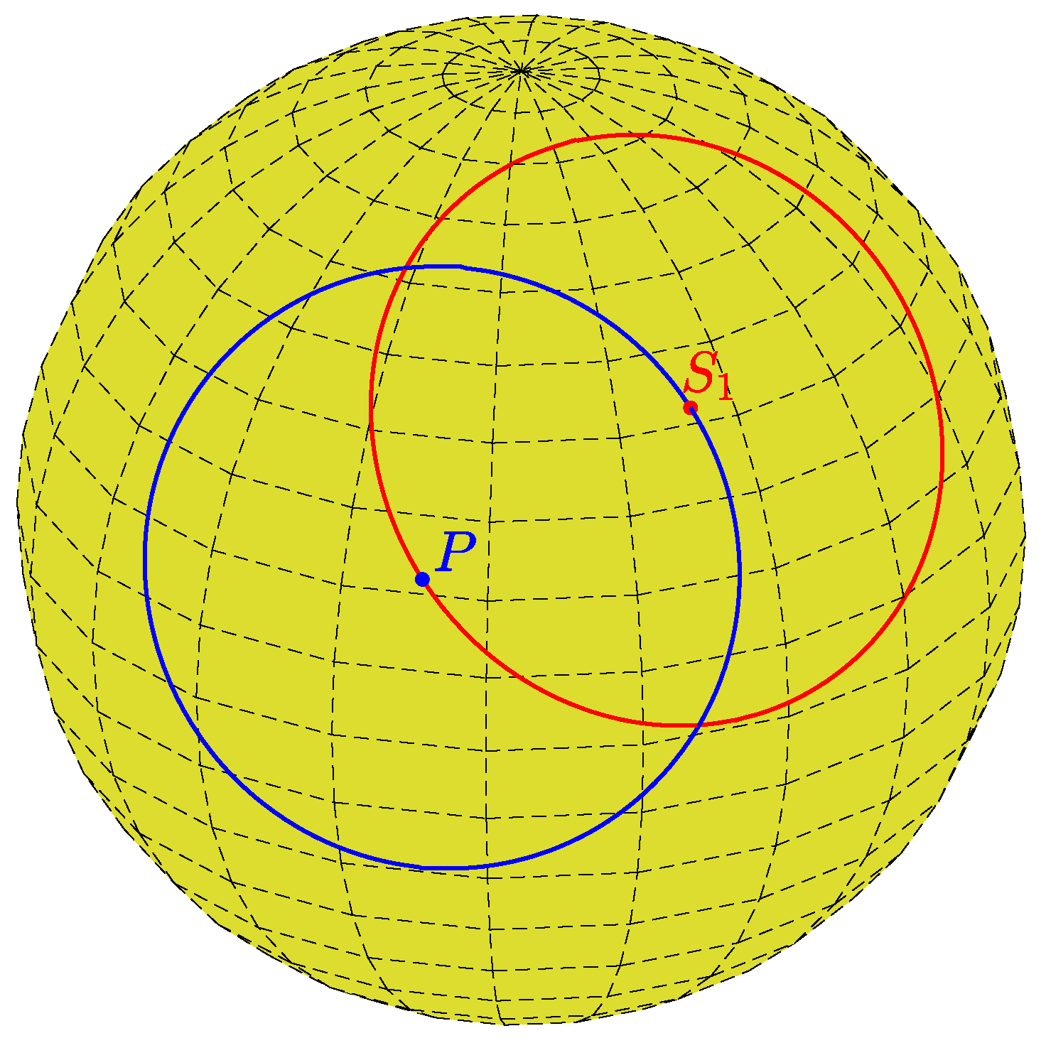
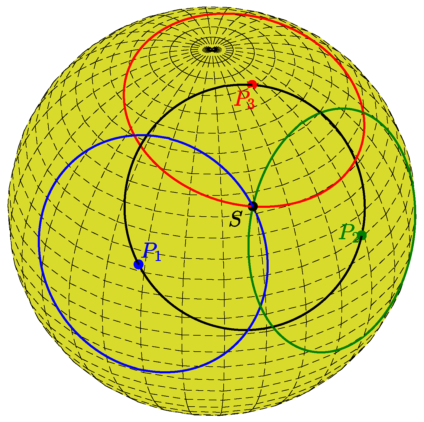
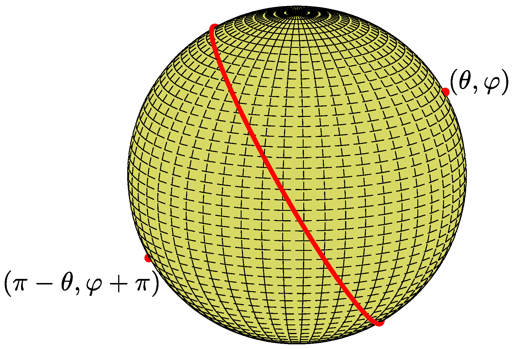
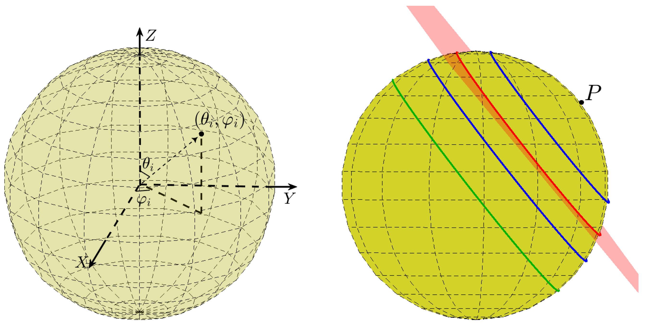
2. Fundamentals
3. The Voting Pattern
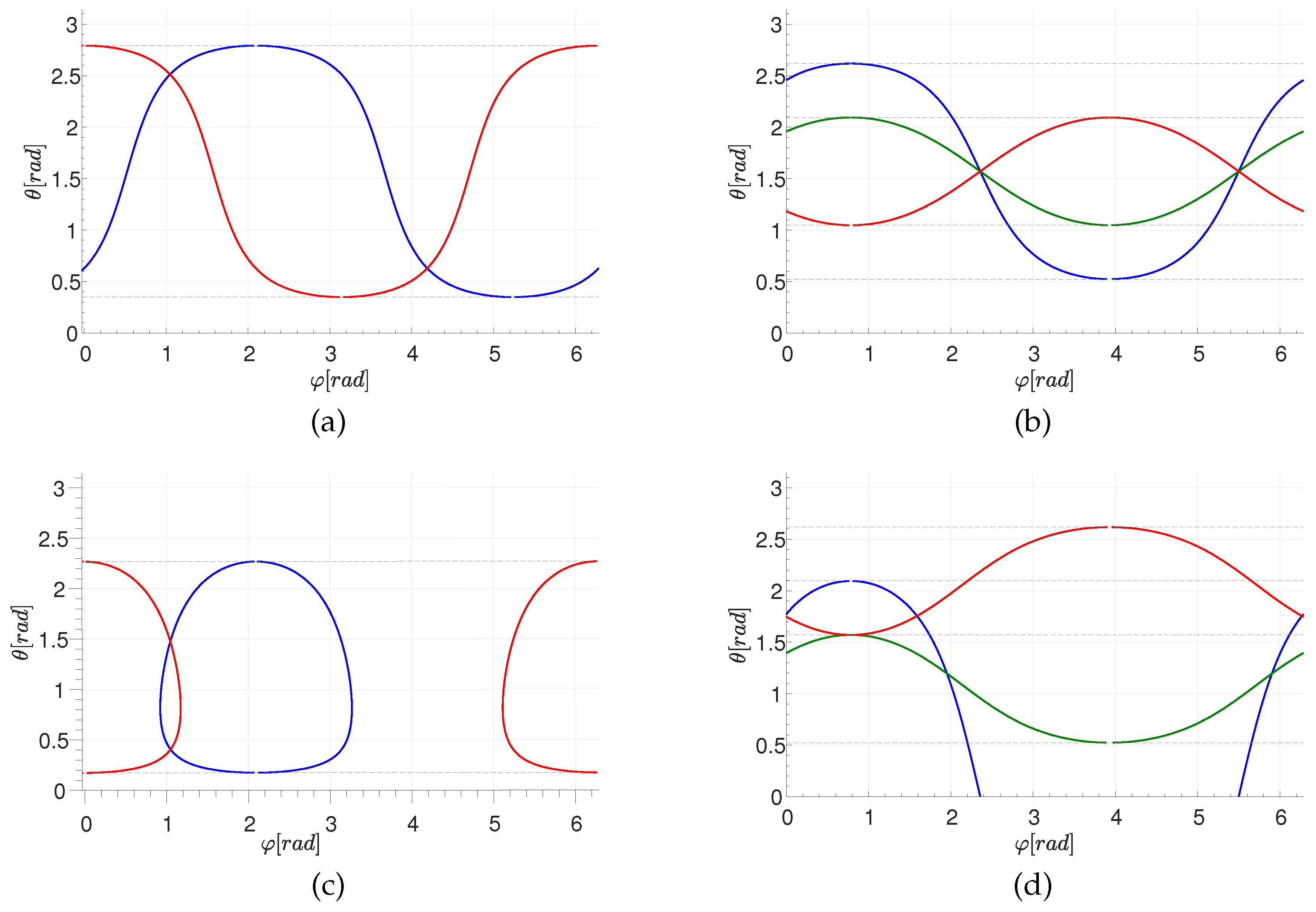
3.1. Derivation of the Voting Pattern
3.2. Domain and Range of the Voting Pattern
3.3. Sphere of Radius R
4. Algorithm for Great-Circle Detection
| Algorithm 1: great-circle detection |
| Initialize the matrix (accumulator array) M with zeros. For each primary point 1 to N For each step Calculate by Equation (10). Round each to the nearest integer multiple of . Increment the accumulator of M corresponding to . Find and corresponding to the entry with the largest accumulation in M. |
5. Algorithm for General (Radius r) Circle Detection on a Sphere
| Algorithm 2: General (any given radius r) circle detection on a sphere |
Initialize the matrix (accumulator array) M with zeros. Normalize the radius r by the sphere radius R. Calculate d by Equation (2). For each primary point 1 to N For each step If satisfies Equation (11) then Calculate and by Equation (8). Round to the nearest integer multiples of . Increment the accumulators of M corresponding to . Find and corresponding to the entry with the largest accumulation in M. |
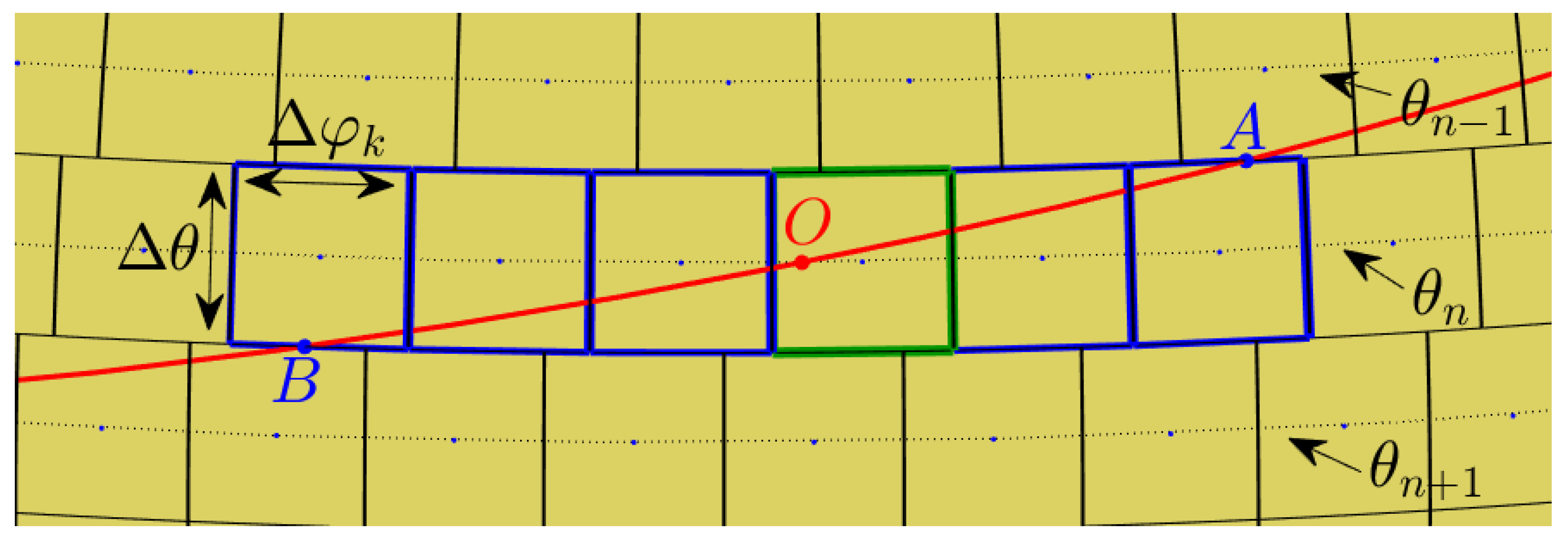
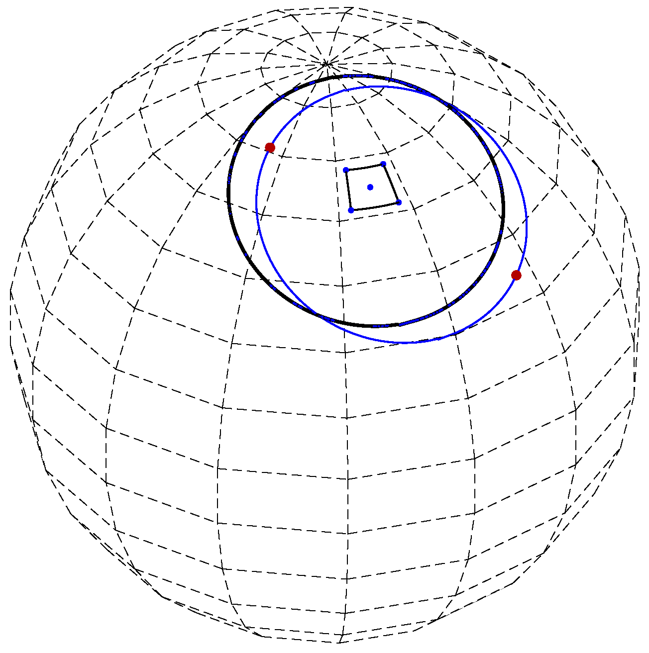
6. Parameter-Space Quantization and Error Analysis
6.1. Preliminaries and Motivation
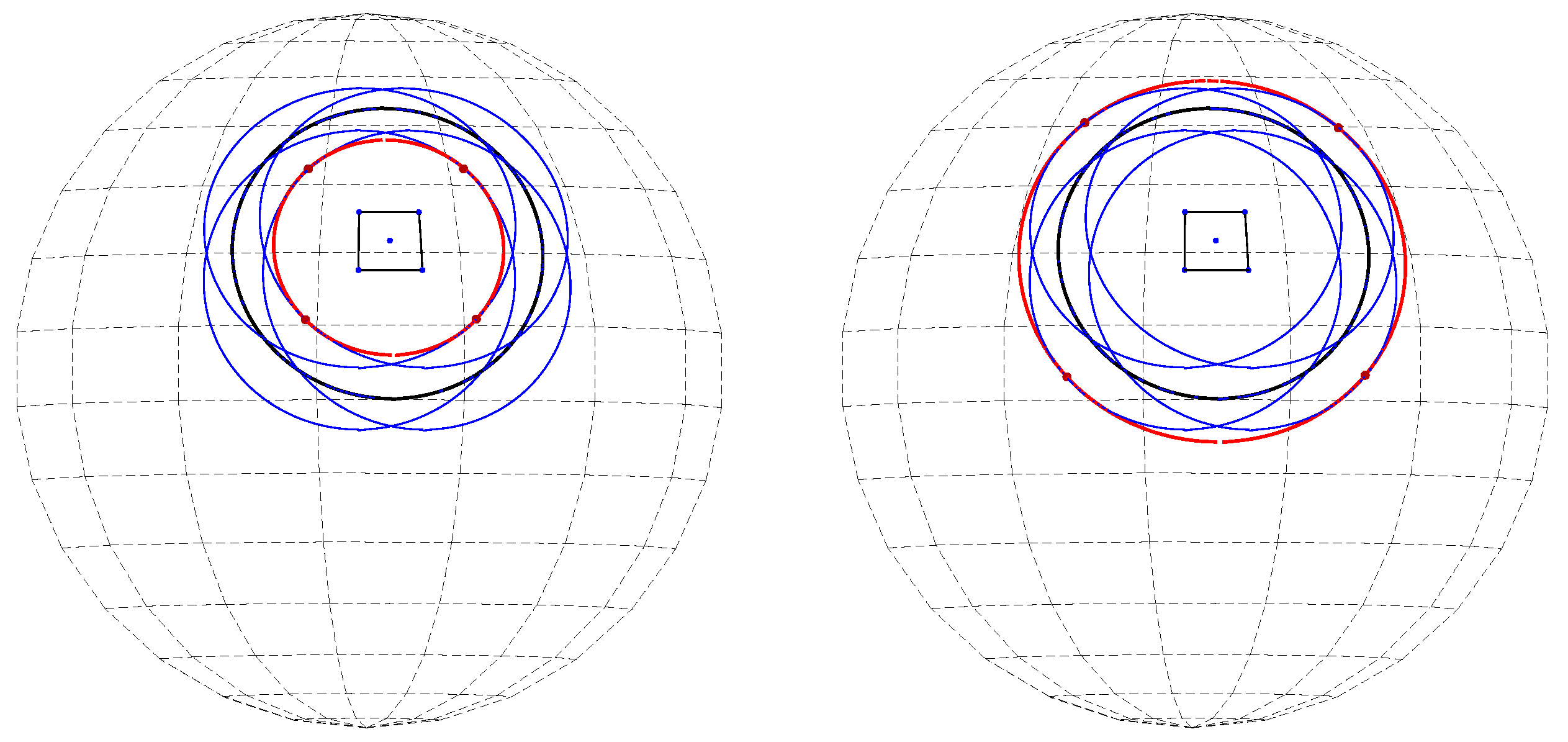
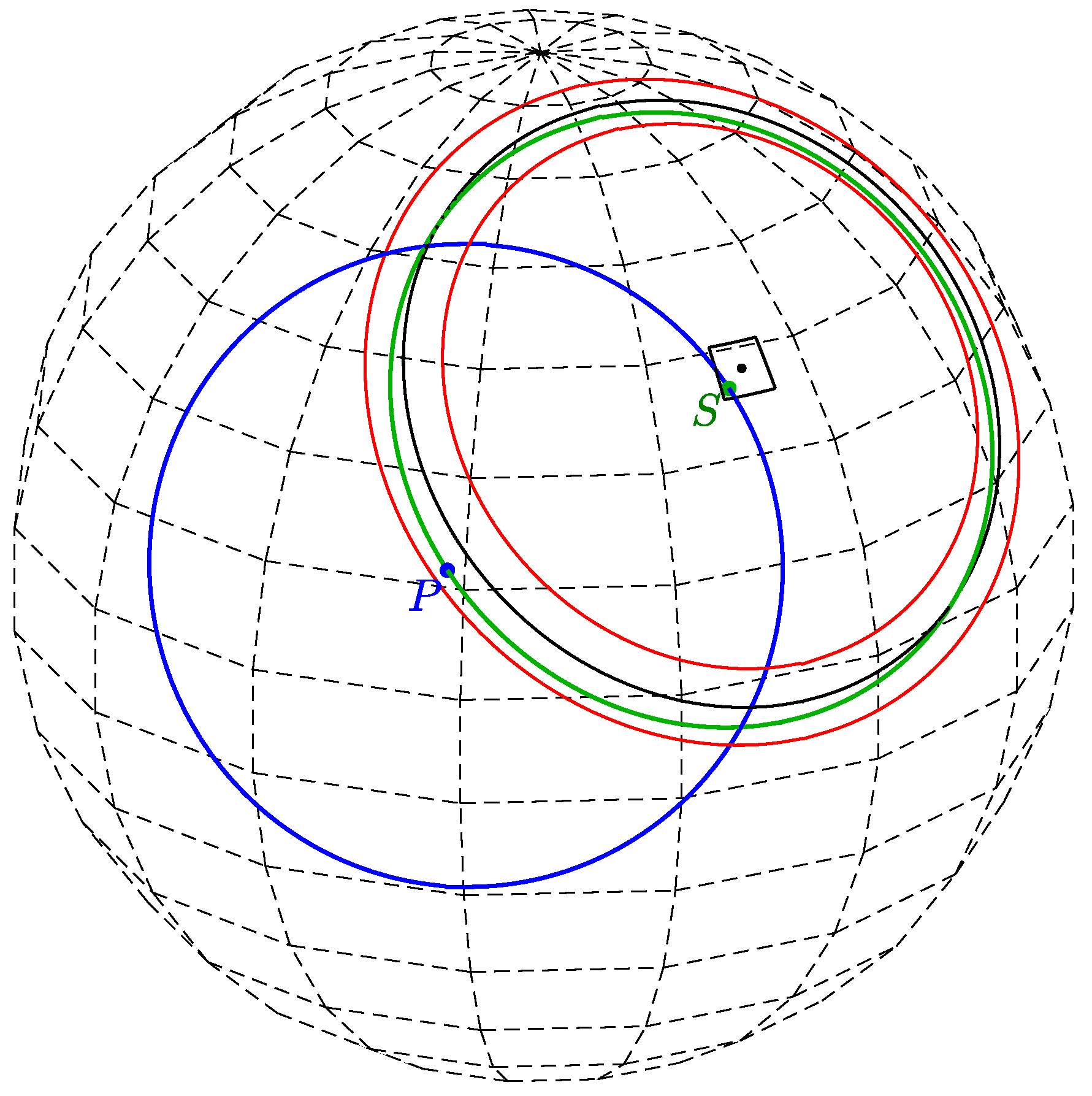
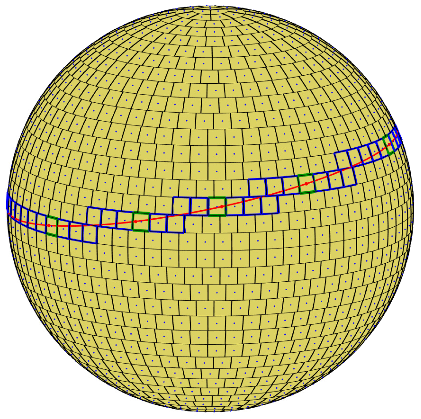
6.2. Towards Uniform Spherical Quantization
6.3. The Distance of Primary Points from the Common Secondary Circle
6.4. Improved Algorithm for General (Radius r) Circle Detection on a Sphere
| Algorithm 3: Improved general circle detection on a sphere |
Initialize the accumulator array M with zeros. Normalize the radius r by the sphere radius R. Calculate d by Equation (2). For each primary point 1 to N Calculate by Equation (12). For each from until : For both and in Equation (8): 1. Calculate by Equation (14). 2. Calculate and by substituting in Equation (8). 3. Choose n such that and 4. Round and to the nearest integer multiples of . 5. Increment the accumulators from to to Find and corresponding to the entry with the largest accumulation in M. |
7. Great Circle Examples
7.1. Uniform Quantization in the Plane (Algorithm 1) Examples
- (1)
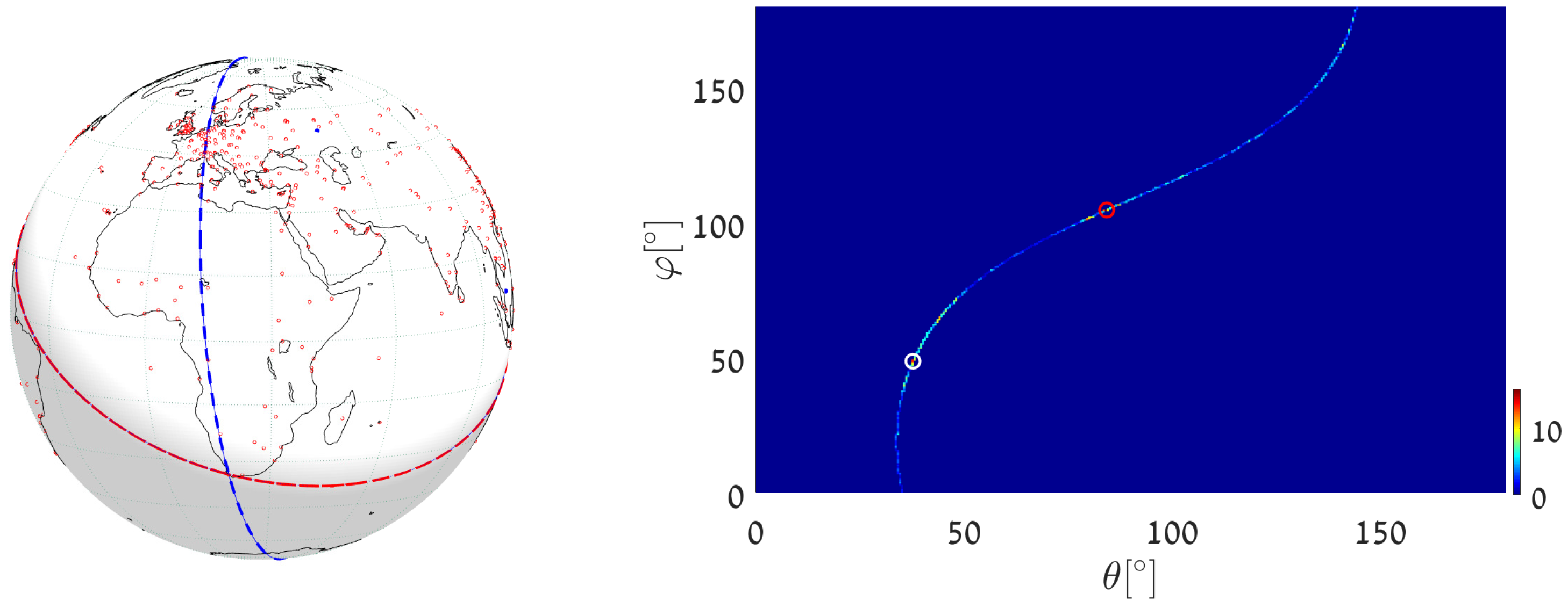
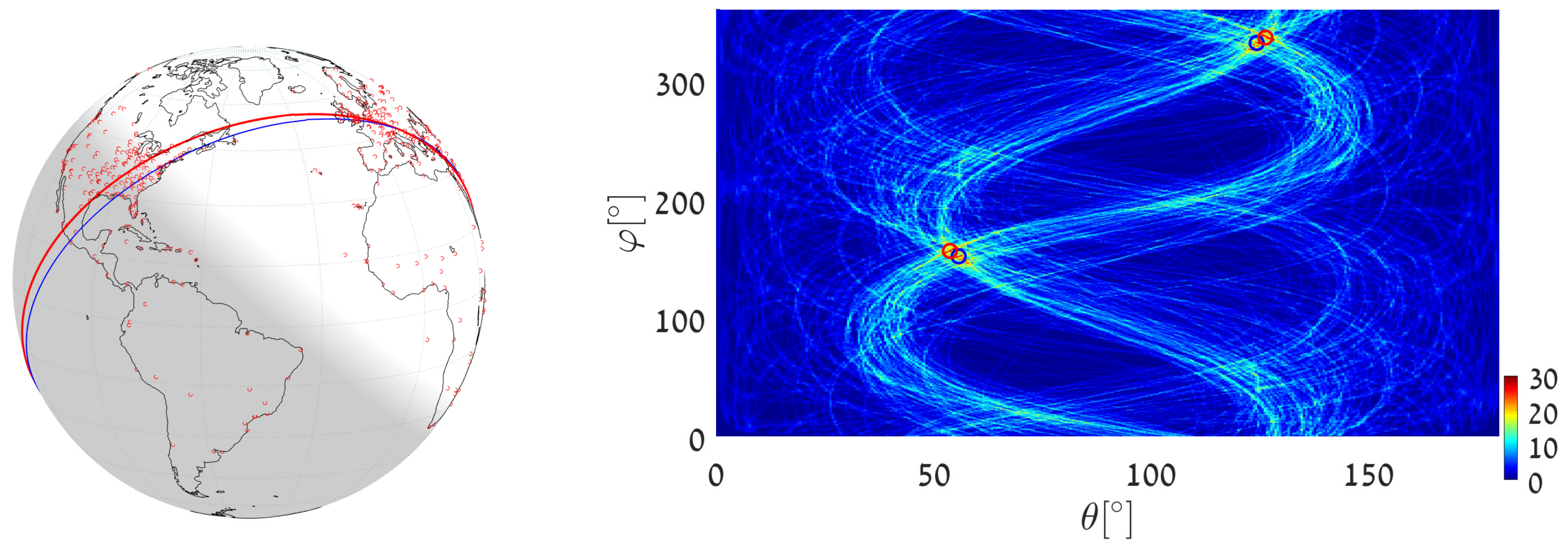
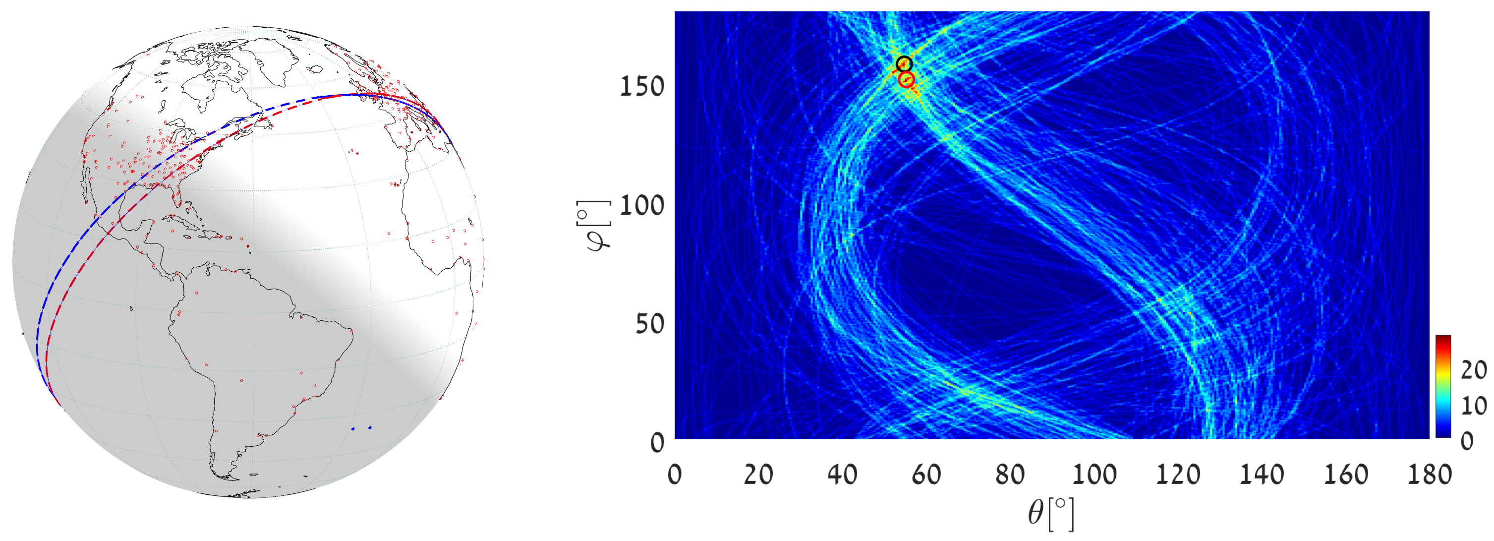
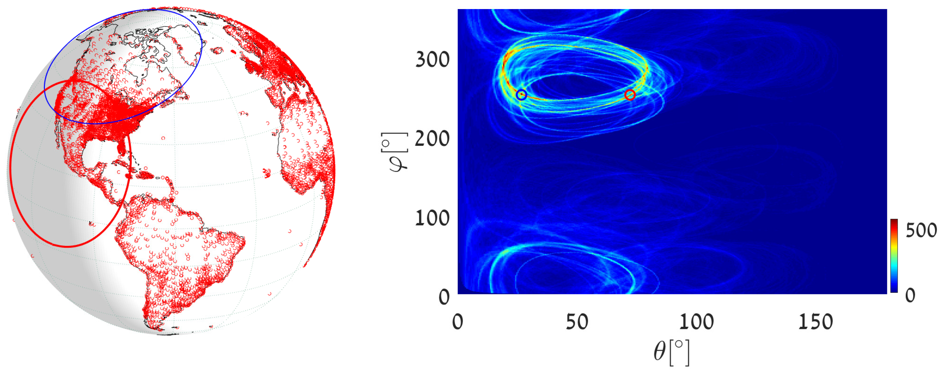
- We execute Algorithm 1, taking the world’s major airports (red dots in Figure 17) as input primary points (a total of 617 points). The parameter space is discretized with . The great circle that passes through the maximum number of airports (blue circle in Figure 17) is on the great circle plane with normal and visits 29 airports, listed in Appendix B. Note that here and in the following, the number of digits after the decimal point in and relates to the location of the cell center. Obviously, the accuracy of the detected circle parameters follows from the cell size, i.e., from and . In order to find the circle passing through the largest number of remaining airports (excluding the 29 airports associated with the first maximum), we identify all primary points of which the voting contributed to the first maximum and remove their votes (unvote [5,6,7]). The new maximum represents the great circle passing through the largest subset of remaining (primary) points in the data-set. It lies on the great circle plane with normal and visits 28 different airports.
- (2)
- We again execute Algorithm 1, this time taking 12,960 world cities (red dots in Figure 18) as input primary points. The parameter space is discretized with . The great circle (blue circle in Figure 18) that passes through the maximum number of cities is on the great circle plane with normal and visits 397 different cities. The great circle that passes through the maximum number of remaining cities (i.e., the maximum after unvoting) is on the great circle plane with normal and visits 321 cities.
- (3)
- We execute the algorithm in order to find the great circle that passes through a specific airport and the maximum number of other airports. Instead of searching for the maximum value in all the accumulators, we search only in accumulators along the curve corresponding to the specific airport. This reduces the computation time, since we search in instead of accumulators.Taking Cape Town International Airport as the specific airport, the great circle that passes through Cape Town International Airport and through the maximum number of other airports is defined by the normal direction (blue circle in Figure 19) and visits 16 different airports, listed in Appendix C. In this case, the discretization of the parameter space is . The great circle that passes through Cape Town International Airport and through the maximum number of remaining airports (the maximum after unvoting, i.e., excluding the airports associated with the first maximum) is on the great circle plane with normal and visits 13 different airports.
7.2. Almost-Equal-Sized Cell Quantization Examples
- (1)
- We execute Algorithm 3 with , taking the world’s major airports as primary input points. We set and , which yields accuracy similar to the worst-case accuracy (at in the above uniform quantization example. The great circle (the blue circle in Figure 20) that passes through the maximum number of airports is on the great circle plane with normal , . It visits 30 different airports, listed in Appendix D. The great circle that passes through the largest number of remaining airports (the maximum after unvoting) is on the great circle plane with and visits 27 airports.
- (2)
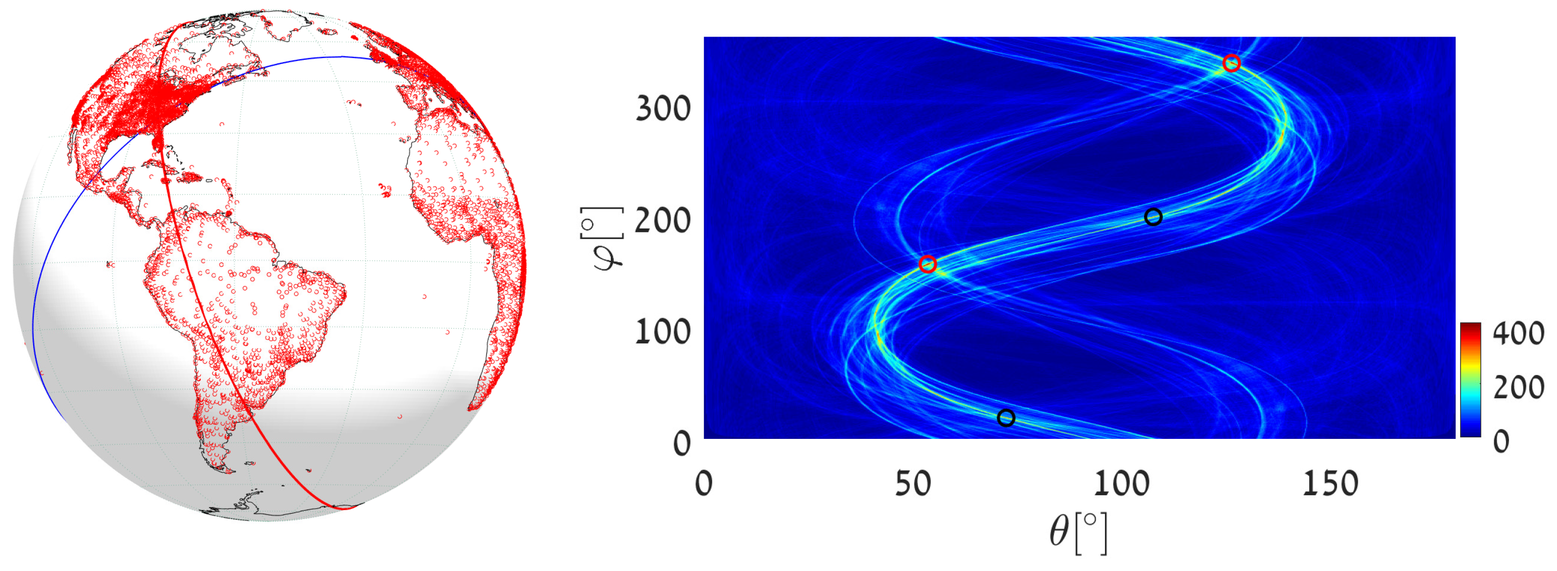
- We execute Algorithm 3 with , taking 12,960 world cities (red dots in Figure 18) as input primary points. We set and . The great circle (the blue circle in Figure 21) that passes through the maximum number of cities is on the great circle plane with normal and visits 425 cities. The great circle that passes through the maximum number of remaining cities (the maximum after unvoting) is on the great circle plane with normal and visits 335 cities.
- (3)
- We execute Algorithm 3 with in order to find the great circle that passes through a specific airport and through the maximum number of other airports. Instead of searching for the maximum value in all the accumulators, we search only in accumulators along the curve corresponding to the specific airport. We again take Cape Town International Airport as the specific airport, now with and . The great circle (the blue circle in Figure 22) that passes through Cape Town International Airport and through the maximum number of other airports is defined by the normal direction , and visits 15 different airports listed in Appendix E. The great circle that passes through the Cape Town International Airport and through the maximum number of remaining airports (the maximum after unvoting, i.e., excluding the airports associated with the first maximum) is on the great circle plane with normal and visits 14 different airports.
8. General (Small) Circle Examples
- (1)
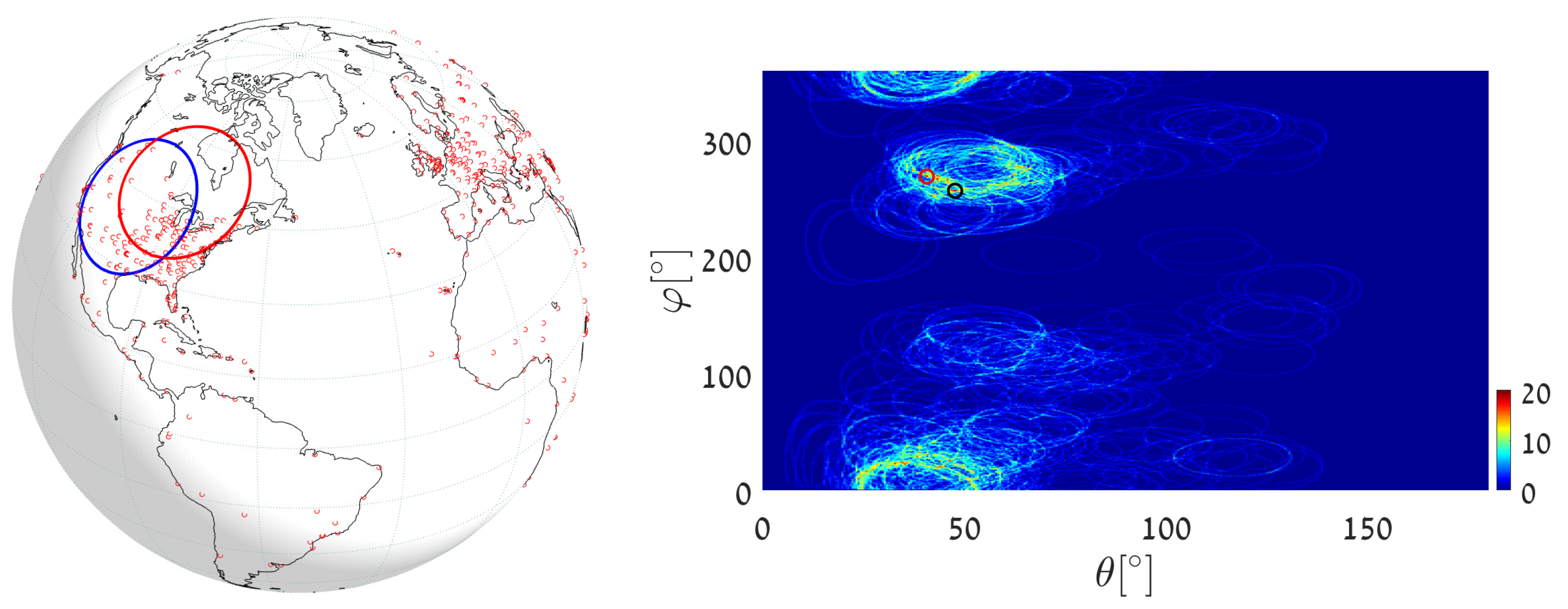
- We execute algorithm 3 with , taking the world’s largest airports as input primary points. We set and . The circle of radius that passes through the maximum number of airports (the blue circle in Figure 24) is on the circle plane with normal and visits 20 large airports. The circle of radius that passes through the largest number of remaining airports (red circle in Figure 24, corresponding to the maximum after unvoting) is on the circle plane with normal , and visits 19 different airports.
- (2)
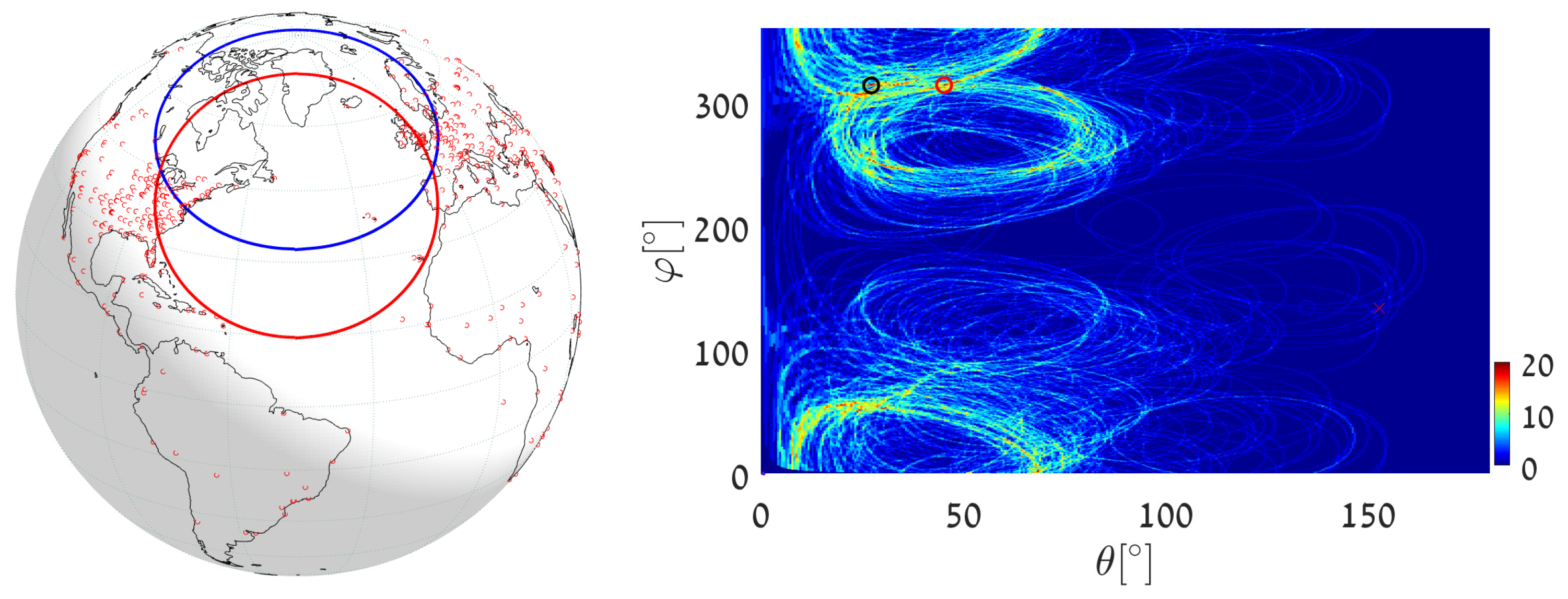
- We now execute algorithm 3 with , again taking the world’s largest airports as input primary points. We set and . The circle of radius that passes through the maximum number of airports (the blue circle in Figure 25) is on the circle plane with normal , and visits 20 large airports. The circle of radius that passes through the largest number of remaining airports (red circle in Figure 25, corresponding to the maximum after unvoting) is on the circle plane with normal and visits 19 different airports.
- (3)
- We execute algorithm 3 with , this time taking the input primary points from the city database. We set and . The circle of radius that passes through the maximum number of cities (the blue circle in Figure 26) is on the circle plane with normal , and visits 616 cities. The circle of radius that passes through the largest number of remaining cities (the black circle in Figure 26, corresponding to the maximum after unvoting) is on the circle plane with normal and visits 386 cities.
- (4)
- We execute algorithm 3, now with , taking the input primary points from the city database. We set and . The circle of radius that passes through the maximum number of cities (the blue circle in Figure 27) is on the circle plane with normal , and visits 568 cities. The circle of radius that passes through the largest number of remaining cities (the black circle in Figure 26, corresponding to the maximum after unvoting) is on the circle plane with normal and visits 523 cities.
9. Conclusions
Author Contributions
Funding
Institutional Review Board Statement
Informed Consent Statement
Data Availability Statement
Conflicts of Interest
Appendix A. Expressing the Angle γ in Terms of ΔS and Δθ
Appendix B. The 29 Airports Located on the Great Circle That Passes through the Maximum Number of Airports—Uniform Quantization
| Airport Name | Latitude | Longitude | ||
| 1 | Prishtina International Airport | 42.572800 | 21.035801 | 0.289202 |
| 2 | Pierre Elliott Trudeau Airport (Montreal) | 45.470600 | −73.740799 | 0.066198 |
| 3 | Brussels South Charleroi Airport | 50.459202 | 4.453820 | 0.108124 |
| 4 | Stuttgart Airport | 48.689899 | 9.221960 | 0.032867 |
| 5 | Karlsruhe Baden-Baden Airport | 48.779400 | 8.080500 | 0.265290 |
| 6 | Luton Airport (London) | 51.874699 | −0.368333 | 0.120182 |
| 7 | Heathrow Airport (London) | 51.470600 | −0.461941 | 0.274561 |
| 8 | Stansted Airport (London) | 51.884998 | 0.235000 | 0.276526 |
| 9 | RAF (Brize Norton) | 51.750000 | −1.583620 | 0.282675 |
| 10 | Findel International Airport (Luxembourg) | 49.623333 | 6.204444 | 0.116230 |
| 11 | Ramstein Air Base | 49.436901 | 7.600280 | 0.153979 |
| 12 | Buffalo Niagara International Airport | 42.940498 | −78.732201 | 0.087453 |
| 13 | John Glenn Columbus International Airport | 39.998001 | −82.891899 | 0.134049 |
| 14 | Corpus Christi International Airport | 27.770399 | −97.501198 | 0.120094 |
| 15 | Cincinnati Northern Kentucky Airport | 39.048801 | −84.667801 | 0.086447 |
| 16 | Erie International Tom Ridge Field | 42.083127 | −80.173867 | 0.101441 |
| 17 | William P Hobby Airport (Houston) | 29.645399 | −95.278900 | 0.141916 |
| 18 | George Bush Intercontinental Airport (Houston) | 29.984400 | −95.341400 | 0.121704 |
| 19 | Rickenbacker International Airport (Columbus) | 39.813801 | −82.927803 | 0.253096 |
| 20 | Memphis International Airport | 35.042400 | −89.976700 | 0.199325 |
| 21 | Monroe Regional Airport | 32.510899 | −92.037697 | 0.292742 |
| 22 | Greater Rochester International Airport | 43.118900 | −77.672401 | 0.256870 |
| 23 | Louisville International Standiford Field | 38.174400 | −85.736000 | 0.020793 |
| 24 | Paphos International Airport | 34.717999 | 32.485699 | 0.020407 |
| 25 | RAF (Akrotiri) | 34.590401 | 32.987900 | 0.189568 |
| 26 | Zagreb Airport | 45.742901 | 16.068800 | 0.085825 |
| 27 | Joe Punik Airport (Ljubljana) | 46.223701 | 14.457600 | 0.158587 |
| 28 | Don Miguel International Airport (Guadalajara) | 20.521799 | −103.310997 | 0.288277 |
| 29 | Queen Alia International Airport (Amman) | 31.722601 | 35.993198 | 0.086299 |
Appendix C. The 16 Airports Located on the Great Circle That Passes through Cape Town and the Maximum Number of Other Airports—Uniform Quantization
| Airport Name | Latitude | Longitude | ||
| 1 | Cape Town International Airport | −33.964802 | 18.601700 | 0.030981 |
| 2 | Tunis Carthage International Airport | 36.851002 | 10.227200 | 0.154490 |
| 3 | Munster Osnabrck Airport | 52.134602 | 7.684830 | 0.227835 |
| 4 | Cologne Bonn Airport | 50.865898 | 7.142740 | 0.310424 |
| 5 | Dortmund Airport | 51.518299 | 7.612240 | 0.085782 |
| 6 | Karlsruhe Baden-Baden Airport | 48.779400 | 8.080500 | 0.045184 |
| 7 | Bergen Airport Flesland | 60.293400 | 5.218140 | 0.307745 |
| 8 | Stavanger Airport Sola | 58.876701 | 5.637780 | 0.247560 |
| 9 | Ramstein Air Base | 49.436901 | 7.600280 | 0.253077 |
| 10 | Hosea Kutako Airport (Windhoek) | −22.479900 | 17.470900 | 0.305683 |
| 11 | Ndjili International Airport (Kinshasa) | −4.385750 | 15.444600 | 0.250095 |
| 12 | Malpensa International Airport (Milan) | 45.630600 | 8.728110 | 0.078630 |
| 13 | Genoa Cristoforo Colombo Airport (Genova) | 44.413300 | 8.837500 | 0.177389 |
| 14 | Milano Linate Airport (Milan) | 45.445099 | 9.276740 | 0.275585 |
| 15 | Zurich Airport (Zurich) | 47.464699 | 8.549170 | 0.067036 |
| 16 | Hammamet International Airport (Enfidha) | 36.075833 | 10.438611 | 0.083588 |
Appendix D. The 30 Airports Located on the Great Circle That Passes through the Maximum Number of Airports—Almost-Equal-Sized Cell Quantization
| Airport Name | Latitude | Longitude | ||
| 1 | South Charleroi Airport (Brussels) | 50.459202 | 4.453820 | 0.154079 |
| 2 | Munich Airport | 48.353802 | 11.786100 | 0.267122 |
| 3 | Stuttgart Airport | 48.689899 | 9.221960 | 0.199825 |
| 4 | Gatwick Airport (London) | 51.148102 | −0.190278 | 0.226057 |
| 5 | Heathrow Airport (London) | 51.470600 | −0.461941 | 0.025712 |
| 6 | RAF (Fairford) | 51.682201 | −1.790030 | 0.026802 |
| 7 | RAF (Brize Norton) | 51.750000 | −1.583620 | 0.076266 |
| 8 | Shannon Airport | 52.702000 | −8.924820 | 0.141270 |
| 9 | Findel International Airport (Luxembourg) | 49.623333 | 6.204444 | 0.177932 |
| 10 | Ramstein Air Base | 49.436901 | 7.600280 | 0.022154 |
| 11 | Joint Base Andrews (Camp Springs) | 38.810799 | −76.866997 | 0.272409 |
| 12 | Hartsfield Jackson Airport (Atlanta) | 33.636700 | −84.428101 | 0.047392 |
| 13 | Asheville Regional Airport | 35.436199 | −82.541801 | 0.251562 |
| 14 | Bradley International Airport (Hartford) | 41.938900 | −72.683197 | 0.156189 |
| 15 | General Edward Logan Airport (Boston) | 42.364300 | −71.005203 | 0.253187 |
| 16 | Thurgood Marshall Airport (Baltimore) | 39.175400 | −76.668297 | 0.093830 |
| 17 | Ronald Reagan Airport (Washington) | 38.852100 | −77.037697 | 0.154835 |
| 18 | Newark Liberty International Airport | 40.692501 | −74.168701 | 0.136928 |
| 19 | Spartanburg International Airport (Greenville) | 34.895699 | −82.218903 | 0.321778 |
| 20 | Washington Dulles International Airport | 38.944500 | −77.455803 | 0.126876 |
| 21 | La Guardia Airport (New York) | 40.777199 | −73.872597 | 0.210181 |
| 22 | Dobbins Air Reserve Base (Marietta) | 33.915401 | −84.516296 | 0.296766 |
| 23 | Montgomery Regional Airport | 32.300598 | −86.393997 | 0.280931 |
| 24 | Mobile Regional Airport | 30.691200 | −88.242798 | 0.310154 |
| 25 | Philadelphia International Airport | 39.871899 | −75.241096 | 0.261567 |
| 26 | Blacksburg Regional Airport (Roanoke) | 37.325500 | −79.975403 | 0.225211 |
| 27 | Sofia Airport | 42.696693 | 23.411436 | 0.204411 |
| 28 | Nikola Tesla Airport (Belgrade) | 44.818401 | 20.309099 | 0.245757 |
| 29 | King Khaled International Airport (Riyadh) | 24.957600 | 46.698799 | 0.135812 |
| 30 | atl | 33.137551 | −84.375000 | 0.338159 |
Appendix E. The 15 Airports Located on the Same Great Circle That Passes through Cape Town and the Maximum Number of Other Airports—Almost-Equal-Sized Cell Quantization
| Airport Name | Latitude | Longitude | ||
| 1 | Cape Town International Airport | −33.964802 | 18.601700 | 0.317152 |
| 2 | Albuquerque International Sunport | 35.040199 | −106.609001 | 0.225185 |
| 3 | Fort Worth Alliance Airport | 32.987598 | −97.318802 | 0.072202 |
| 4 | Cannon Air Force Base (Clovis) | 34.382801 | −103.321999 | 0.143119 |
| 5 | Dallas Love Field (Dallas) | 32.847099 | −96.851799 | 0.072541 |
| 6 | Dallas Fort Worth International Airport | 32.896801 | −97.038002 | 0.066215 |
| 7 | Hollywood Airport (Fort Lauderdale) | 26.072599 | −80.152702 | 0.147474 |
| 8 | Meacham International Airport (Fort Worth) | 32.819801 | −97.362396 | 0.098141 |
| 9 | Biloxi International Airport (Gulfport) | 30.407301 | −89.070099 | 0.286861 |
| 10 | Metropolitan Oakland International Airport | 37.721298 | −122.221001 | 0.268331 |
| 11 | San Francisco International Airport | 37.618999 | −122.375000 | 0.155643 |
| 12 | Norman Y. Mineta Airport (San Jose) | 37.362598 | −121.929001 | 0.067841 |
| 13 | Sarasota Bradenton International Airport | 27.395399 | −82.554398 | 0.029516 |
| 14 | Lynden Pindling Airport (Nassau) | 25.039000 | −77.466202 | 0.112437 |
| 15 | Luis Munoz Marin Airport (San Juan) | 18.439400 | −66.001801 | 0.061461 |
Appendix F. The Dependence of the Number of Points Associated with the Great Circle Detected on the Parameter Space Quantization Level
| Dataset | Quantization | Number of Points | Parameters of the | ||
| Level | Associated with the | Great Circle Detected | |||
| (Degrees) | Great Circle Detected | (Degrees) | |||
| Cities | 2 | 1703 | 156.2500 | 53 | |
| 1 | 1177 | 155.7093 | 53.5000 | ||
| 0.5 | 729 | 156.4544 | 53.7500 | ||
| 0.25 | 425 | 156.3934 | 53.625 | ||
| 0.2 | 359 | 156.4300 | 53.7000 | ||
| 0.1 | 198 | 155.7920 | 53.2500 | ||
| 0.05 | 120 | 145.0215 | 48.0750 | ||
| Airports | 2 | 78 | 156.2500 | 53 | |
| 1 | 50 | 157.8840 | 54.5000 | ||
| 0.5 | 30 | 156.4544 | 53.7500 | ||
| 0.25 | 19 | 150.7367 | 55.1250 | ||
| 0.166 | 15 | 154.3911 | 52.2500 | ||
| 0.125 | 13 | 155.7198 | 53.4375 | ||
| 0.1 | 12 | 151.2559 | 55.3500 | ||
| 0.05 | 10 | 154.8403 | 56.1750 | ||
| Airports through Cape Town | 2 | 39 | 49.3805 | 39 | |
| 1 | 24 | 49.3151 | 37.5000 | ||
| 0.5 | 15 | 49.3878 | 37.7500 | ||
| 0.25 | 10 | 49.0724 | 37.8750 | ||
References
- Fischler, M.A.; Bolles, R.C. Random Sample Consensus: A paradigm for model fitting with applications to image analysis and Automated Cartography. Commun. Assoc. Comput. Mach. ACM 1981, 24, 381–396. [Google Scholar] [CrossRef]
- Duda, R.O.; Hart, P.E. Use of the Hough transformation to detect lines and curves in pictures. Commun. Assoc. Comput. Mach. ACM 1972, 15, 11–15. [Google Scholar] [CrossRef]
- Kiryati, N.; Bruckstein, A.M. Heteroscedastic Hough Transform (HtHT): An efficient Method for Robust Line Fittingin the ‘Errors in the Variables’ Problem. Comput. Vis. Image Underst. 2000, 78, 69–83. [Google Scholar] [CrossRef]
- López-González, G.; Arana-Daniel, N.; Bayro-Corrochano, E. Conformal Hough Transform for 2D and 3D Cloud Points. In Progress in Pattern Recognition, Image Analysis, Computer Vision, and Applications (CIARP 2013), Lecture Notes in Computer Science; Ruiz-Shulcloper, J., di Baja, G.S., Eds.; Springer: Berlin/Heidelberg, Germany, 2013; Volume 8258. [Google Scholar]
- Gerig, G.; Klein, F. Fast contour identification through efficient Hough Transform and simplified interpretation strategy. In Proceedings of the International Conference on Pattern Recognition (ICPR), Paris, France, 27–31 October 1986; pp. 498–500. [Google Scholar]
- Gerig, G. Linking image-space and accumulator-space: A new approach for object recognition. In Proceedings of the 1st International Conference on Computer Vision (ICCV), London, UK, 8–14 June 1987; pp. 112–117. [Google Scholar]
- Matas, J.; Galambos, C.; Kittler, J. Progressive Probabilistic Hough Transform. In Proceedings of the British Machine Vision Conference (BMVC), Southampton, UK, 14–17 September 1998; pp. 26.1–26.10. [Google Scholar]
- Vasseur, P.; Moaddib, E.-M. Central Catadioptric Line Detection. In Proceedings of the British Machine Vision Conference (BMVC), London, UK, 7–9 September 2004. [Google Scholar]
- Torii, A.; Imiya, A. The randomized-Hough-transform-based method for great-circle detection on sphere. Pattern Recognit. Lett. 2007, 28, 1186–1192. [Google Scholar] [CrossRef]
- Boutteau, R.; Savatier, X.; Bonardi, F.; Ertaud, J.-Y. Road-line detection and 3D reconstruction using fisheye cameras. In Proceedings of the IEEE 16th International Conference on Intelligent Transportation Systems (ITSC), The Hague, The Netherlands, 6–9 October 2013. [Google Scholar]
- Barnard, S.T. Interpreting perspective images. Artif. Intell. 1983, 21, 435–462. [Google Scholar] [CrossRef]
- Quan, L.; Mohr, R. Determining persepctive structures using hierarchical Hough transform. Pattern Recognit. Lett. 1989, 9, 279–286. [Google Scholar] [CrossRef]
- Lutton, E.; Maitre, H.; Lopez-Krahe, J. Contribution to the determination of vanishing points using Hough transform. IEEE Trans. Pattern Anal. Mach. Intell. 1994, 16, 430–438. [Google Scholar] [CrossRef]
- Ying, X.; Hu, Z. Catadioptric line features detection using Hough transform. In Proceedings of the 17th International Conference on Pattern Recognition (ICPR), Cambridge, UK, 26 August 2004; Volume 4, pp. 839–842. [Google Scholar]
- Ericson, S.; Astrand, B. Row-detection on an agricultural field using omnidirectional camera. In Proceedings of the IEEE/RSJ International Conference on Intelligent Robots and Systems, Taipei, Taiwan, 18–22 October 2010. [Google Scholar]
- Pacey, A.; Macpherson, C.G.; McCaffrey, K.J.W. Linear volcanic segments in the central Sunda Arc, Indonesia, identified using Hough Transform analysis: Implications for arc lithosphere control upon volcano distribution. Earth Planet. Sci. Lett. 2013, 369–370, 24–33. [Google Scholar] [CrossRef] [Green Version]
- Andikagumi, H.; Macpherson, C.G.; McCaffrey, K.J.W. Upper plate stress controls the distribution of Mariana arc volcanoes. J. Geophys. Res. Solid Earth 2020, 125, e2019JB017391. [Google Scholar] [CrossRef]
- Wessel, P. Hotspotting: Principles and properties of a plate tectonic Hough transform. Geochem. Geophys. Geosyst. 2008, 9, Q08004. [Google Scholar] [CrossRef]
- Snyder, J.P. Flattening the Earth: Two Thousand Years of Map Projections; The University of Chicago Press: Chicago, IL, USA, 1993. [Google Scholar]
- Klette, R.; Rosenfeld, A. Digital Geometry: Geometric Methods for Digital Picture Analysis; (Section 1.1.4); Elsevier: Amsterdam, The Netherlands, 2004. [Google Scholar]
- Koplowitz, J. On the performance of chain codes for quantization of line drawings. IEEE Trans. Pattern Anal. Mach. Intell. PAMI 1981, 3, 181–185. [Google Scholar] [CrossRef] [PubMed]
- Kiryati, N.; Lindenbaum, M.; Bruckstein, A.M. Digital or analog Hough transform? Pattern Recognit. Lett. 1991, 12, 291–297. [Google Scholar] [CrossRef] [Green Version]
- Santalo, L. Integral Geometry and Geometric Probability. In Encyclopedia of Mathematics and Its Applications; Addison-Wesley: Boston, MA, USA, 1976; Volume 1. [Google Scholar]
- World Cities Coordinates Data Set. Available online: https://simplemaps.com/data/world-cities (accessed on 14 October 2019).
- Airports Coordinates Data Set. Available online: https://www.partow.net/miscellaneous/airportdatabase/ (accessed on 14 October 2019).


| Dataset | Algorithm 1 | Algorithm 3 | ||||||
|---|---|---|---|---|---|---|---|---|
| Δθ | Δφ | Computing Time (ms) | Δθ | ΔS | Computing Time (ms) | |||
| Total Time | Avg. per Point | Total Time | Avg. per Point | |||||
| Airports | 2 | 2 | 366 | 0.43 | 2 | 595 | 0.93 | |
| 1 | 1 | 531 | 0.71 | 1 | 791 | 1.33 | ||
| 0.5 | 0.5 | 1298 | 1.98 | 0.5 | 1777 | 3.02 | ||
| (616 pts.) | 0.25 | 0.25 | 3321 | 5.16 | 0.25 | 3668 | 5.96 | |
| Cities | 2 | 2 | 3644 | 0.29 | 2 | 6755 | 0.53 | |
| 1 | 1 | 6174 | 0.47 | 1 | 10,225 | 0.75 | ||
| 0.5 | 0.5 | 22,779 | 1.64 | 0.5 | 26,231 | 2.07 | ||
| (12,959 pts.) | 0.25 | 0.25 | 64,385 | 5.02 | 0.25 | 72,061 | 5.56 | |
| Cities | - | - | - | - | 2 | 5972 | 0.48 | |
| - | - | - | - | 1 | 8343 | 0.70 | ||
| - | - | - | - | 0.5 | 23,403 | 1.98 | ||
| (12,959 pts.) | - | - | - | - | 0.25 | 64,078 | 4.97 | |
| Cities | - | - | - | - | 2 | 5562 | 0.43 | |
| - | - | - | - | 1 | 7630 | 0.57 | ||
| - | - | - | - | 0.5 | 22,423 | 1.71 | ||
| (12,959 pts.) | - | - | - | - | 0.25 | 58,805 | 4.53 | |
Publisher’s Note: MDPI stays neutral with regard to jurisdictional claims in published maps and institutional affiliations. |
© 2022 by the authors. Licensee MDPI, Basel, Switzerland. This article is an open access article distributed under the terms and conditions of the Creative Commons Attribution (CC BY) license (https://creativecommons.org/licenses/by/4.0/).
Share and Cite
Ibrahim, B.; Kiryati, N. Detecting Cocircular Subsets of a Spherical Set of Points. J. Imaging 2022, 8, 184. https://doi.org/10.3390/jimaging8070184
Ibrahim B, Kiryati N. Detecting Cocircular Subsets of a Spherical Set of Points. Journal of Imaging. 2022; 8(7):184. https://doi.org/10.3390/jimaging8070184
Chicago/Turabian StyleIbrahim, Basel, and Nahum Kiryati. 2022. "Detecting Cocircular Subsets of a Spherical Set of Points" Journal of Imaging 8, no. 7: 184. https://doi.org/10.3390/jimaging8070184
APA StyleIbrahim, B., & Kiryati, N. (2022). Detecting Cocircular Subsets of a Spherical Set of Points. Journal of Imaging, 8(7), 184. https://doi.org/10.3390/jimaging8070184