
Object Categorization Capability of Psychological Potential Field in Perceptual Assessment Using Line-Drawing Images


Abstract
1. Introduction
2. Fixation Maps
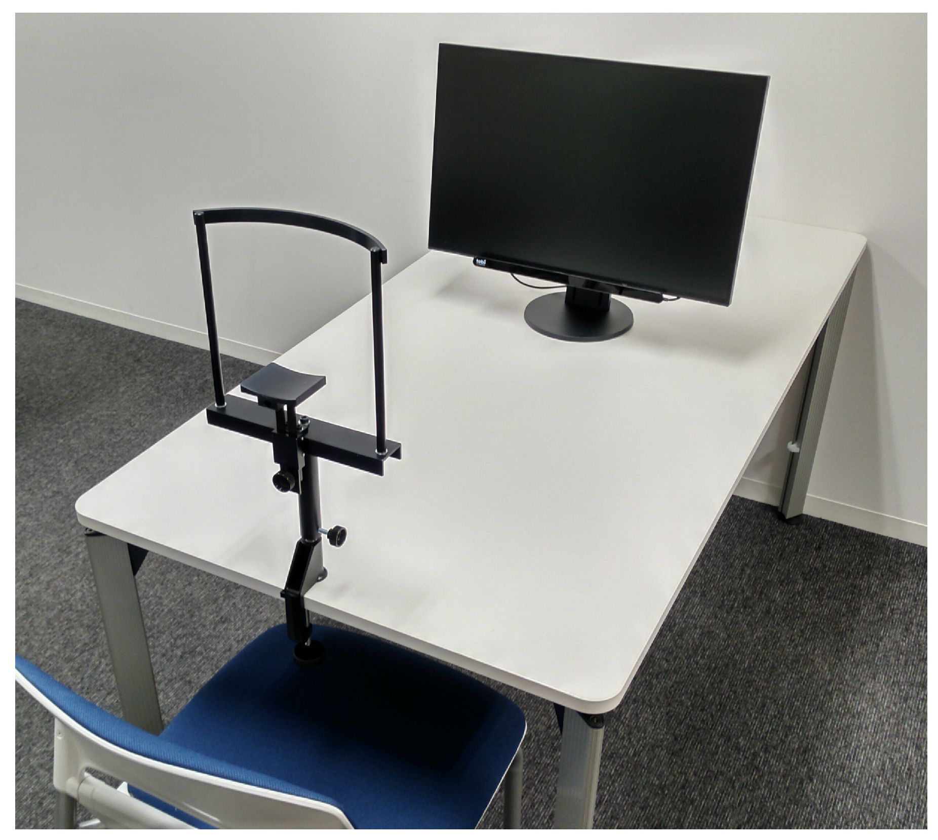
2.1. Eye Tracking
2.2. Fixation Map Generation
3. Image Features and Similarity Metric
3.1. Stimulus Images and Experimental Setups
3.2. Image Features and Similarity Metric
3.2.1. Fundamental Similarity Metric
3.2.2. Binary Feature
3.2.3. Reciprocal Distance Field
3.2.4. BIN + RDF
3.2.5. Psychological Potential Field
4. Results
5. Discussion
6. Conclusions
Author Contributions
Funding
Institutional Review Board Statement
Informed Consent Statement
Data Availability Statement
Conflicts of Interest
References
- Lahmiri, S. An Accurate System to Distinguish Between Normal and Abnormal Electroencephalogram Records with Epileptic Seizure Free Intervals. Biomed. Signal Process. Control 2018, 40, 312–317. [Google Scholar] [CrossRef]
- Burch, M. Visual Analysis of Eye Movement Data with Fixation Distance Plots. Intell. Decis. Technol. 2017, 73, 227–236. [Google Scholar]
- Walther, D.B.; Chai, B.; Caddigan, E.; Beck, D.M.; Fei-Fei, L. Simple Line Drawings Suffice for Functional MRI Decoding of Natural Scene Categories. Proc. Natl. Acad. Sci. USA 2011, 108, 9661–9666. [Google Scholar] [CrossRef] [PubMed]
- Fu, Q.; Liu, Y.J.; Dienes, Z.; Wu, J.; Chen, W.; Fu, X. Neural Correlates of Subjective Awareness for Natural Scene Categorization of Color Photographs and Line-drawings. Front. Psychol. 2017, 8, 210. [Google Scholar] [CrossRef] [PubMed]
- Awano, N.; Hayashi, Y. Psychological Potential Field and Human Eye Fixation on Binary Line-drawing Images: A Comparative Experimental Study. Comput. Vis. Media 2020, 6, 205–214. [Google Scholar] [CrossRef]
- Yokose, Z. A Study on Character-Patterns Based Upon the Theory of Psychological Potential Field. Jpn. Psychol. Res. 1970, 12, 18–25. [Google Scholar] [CrossRef]
- Ichikawa, N. The measurement of the figure-effect in the third dimension by the light threshold method. Jpn. J. Psychol. 1967, 38, 274–283. [Google Scholar] [CrossRef]
- Kaji, S.; Yamane, S.; Yoshimura, M.; Sugie, N. Contour enhancement of two-dimensional figures observed in the lateral geniculate cells of cats. Vis. Res. 1974, 14, 113–117. [Google Scholar] [CrossRef]
- Fukouzu, Y.; Itoh, A.; Yoshida, T.; Shiraishi, T. An analysis of the figure by the visual space transfer model: A study on elucidation and estimation of a scene on figure recognition (6). Bull. Jpn. Soc. Sci. Des. 1998, 45, 75–82. [Google Scholar]
- Motokawa, K. Psychology and Physiology of Vision. J. Inst. Telev. Eng. Jpn. 1962, 16, 425–431. [Google Scholar]
- Kimch, R.; Hadad, B.S. Influence of Past Experience on Perceptual Grouping. Psychol. Sci. 2002, 13, 41–47. [Google Scholar] [CrossRef] [PubMed]
- Schwabe, K.; Menzel, C.; Mullin, C.; Wagemans, J.; Redies, C. Gist Perception of Image Composition in Abstract Artworks. i-Perception 2018, 9, 1–25. [Google Scholar] [CrossRef] [PubMed]
- Miyoshi, M.; Shimoshio, Y.; Koga, H. Automatic lettering design based on human kansei. In Proceedings of the International Conference on Human—Computer Interaction, Las Vegas, NV, USA, 22–27 July 2005. [Google Scholar]
- Onaga, H.; Fukouzu, Y.; Yoshida, T.; Shiraishi, T. Relation between potential and curvature optical illusion: A study on elucidation and estimation of a scene on figure recognition (report 5). Bull. Jpn. Soc. Sci. Des. 1996, 43, 77–84. [Google Scholar]
- Awano, N.; Morohoshi, K. Objective evaluation of impression of faces with various female hairstyles using field of visual perception. IEICE Trans. Inf. Syst. 2018, 101, 1648–1656. [Google Scholar] [CrossRef]
- Borji, A.; Itti, L. CAT2000: A Large Scale Fixation Dataset for Boosting Saliency Research. arXiv 2015, arXiv:1505.03581. [Google Scholar]
- Awano, N. Acceleration of Calculation for Field of Visual Perception on Digital Image and Verification of the Application to Halftone Image. Trans. Jpn. Soc. Kansei Eng. 2017, 16, 209–218. [Google Scholar] [CrossRef]
- Awano, N.; Akiyama, M.; Muraki, Y.; Kobori, K. Complexity Analysis of Psychological Potential Field for Quantification of Hairstyle for Facial Impression. Trans. Jpn. Soc. Kansei Eng. 2020, 19, 335–342. [Google Scholar] [CrossRef]
- Felzenszwalb, P.F.; Huttenlocher, D.P. Distance Transforms of Sampled Functions. Theory Comput. 2012, 8, 415–428. [Google Scholar] [CrossRef]
- Eckstein, M.K.; Guerra-Carrillo, B.; Singley, A.T.M.; Bunge, S.A. Beyond Eye Gaze: What Else Can Eyetracking Reveal about Cognition and Cognitive Development? Dev. Cogn. Neurosci. 2017, 25, 69–91. [Google Scholar] [CrossRef]
- Harezlak, K.; Kasprowski, P. Application of Eye Tracking in Medicine: A survey, Research Issues and Challenges. Comput. Med. Imaging Graph. 2018, 65, 176–190. [Google Scholar] [CrossRef]
- Alghowinem, S.; Goecke, R.; Wagner, M.; Parker, G.; Breakspear, M. Eye Movement Analysis for Depression Detection. In Proceedings of the IEEE International Conference on Image Processing, Melbourne, Australia, 15–18 September 2013; pp. 4220–4224. [Google Scholar]
- Majaranta, P.; Bulling, A. Eye Tracking and Eye-Based Human–Computer Interaction, Chapter 3, Advances in Physiological Computing; Fairclough, S., Gilleade, K., Eds.; Springer: London, UK, 2014; pp. 39–65. [Google Scholar]
- Ogino, R.; Hayashi, Y.; Seta, K. A Sustainable Training Method of Metacognitive Skills in Daily Lab Activities Using Gaze-aware Reflective Meeting Reports. J. Inf. Syst. Educ. 2019, 18, 16–26. [Google Scholar] [CrossRef]
- Learn about the Different Types of Eye Movement. Available online: https://www.tobiipro.com/learn-and-support/learn/eye-tracking-essentials/types-of-eye-movements/ (accessed on 12 February 2022).
- Courtemanche, F.; Léger, P.M.; Dufresne, A.; Fredette, M.; Labonté-Lemoyne, É.; Sénécal, S. Physiological Heatmaps: A Tool for Visualizing Users’ Emotional Reactions. Multimed. Tools Appl. 2018, 77, 11547–11574. [Google Scholar] [CrossRef]
- Holmqvist, K.; Nystrom, M.; Andersson, R.; Dewhurst, R.; Jarodzka, H.; Weijer, J.V.D. Eye Tracking: A Comprehensive Guide to Methods and Measures; Oxford University Press: New York, NY, USA, 2011. [Google Scholar]
- Kroner, A.; Senden, M.; Driessens, K.; Goebel, R. Contextual Encoder-Decoder Network for Visual Saliency Prediction. Neural Netw. 2020, 129, 261–270. [Google Scholar] [CrossRef] [PubMed]
- Kümmerer, M.; Wallis, T.S.A.; Gatys, L.A.; Bethge, M. Understanding Low- and High-Level Contributions to Fixation Prediction. In Proceedings of the IEEE International Conference on Computer Vision, Venice, Italy, 22–29 October 2017; pp. 4789–4798. [Google Scholar]
- Papoutsaki, A.; James, L.; Huang, J. SearchGazer: Webcam Eye Tracking for Remote Studies of Web Search. In Proceedings of the Conference on Human Information Interaction and Retrieval, Oslo, Norway, 7–11 March 2017; pp. 17–26. [Google Scholar]
- Tavakoli, H.R.; Ahmed, F.; Borji, A.; Laaksonen, J. Saliency Revisited: Analysis of Mouse Movements Versus Fixations. In Proceedings of the IEEE Conference on Computer Vision and Pattern Recognition, Honolulu, HI, USA, 21–26 July 2017; pp. 6354–6362. [Google Scholar]
- Kim, N.W.; Bylinskii, Z.; Borkin, M.A.; Gajos, K.Z.; Oliva, A.; Durand, F.; Pfister, H. BubbleView: An Interface for Crowdsourcing Image Importance Maps and Tracking Visual Attention. ACM Trans. Comput.-Hum. Interact. 2017, 24, 1–40. [Google Scholar] [CrossRef]
- MIT/Tübingen Saliency Benchmark Datasets. Available online: https://saliency.tuebingen.ai/datasets.html (accessed on 31 January 2022).
- Aramaki, E.; Nakamura, T.; Usuda, Y.; Kubo, K.; Miyabe, M. Naming of Meaningless Sketch Image. SIG-AM 2013, 5, 47–51. [Google Scholar]
- Borji, A.; Sihite, D.N.; Itti, L. Quantitative Analysis of Human-model Arrangement in Visual Saliency Modeling: A Comparative Study. IEEE Trans. Image Process. 2013, 22, 55–69. [Google Scholar] [CrossRef]
- Peters, R.J.; Iyer, A.; Itti, L.; Koch, C. Components of Bottom-up Gaze Allocation in Natural Images. Vis. Res. 2005, 45, 2397–2416. [Google Scholar] [CrossRef]
- Kümmerer, M.; Wallis, T.S.A.; Bethge, M. Information-theoretic Model Comparison Unifies Saliency Metrics. Proc. Natl. Acad. Sci. USA 2015, 112, 16054–16059. [Google Scholar] [CrossRef]
- Riche, N.; Duvinage, M.; Mancas, M.; Gosselin, B.; Dutoit, T. Saliency and Human Fixations: State-of-theart and Study of Comparison Metrics. In Proceedings of the IEEE International Conference on Computer Vision, Sydney, NSW, Australia, 1–8 December 2013; pp. 1153–1160. [Google Scholar]
- Bylinskii, Z.; Judd, T.; Oliva, A.; Torralba, A.; Durand, F. What Do Different Evaluation Metrics Tell Us About Saliency Models? IEEE Trans. Pattern Anal. Mach. Intell. 2019, 41, 740–757. [Google Scholar] [CrossRef]
- Zhu, W.N.; Drewes, J.; Peatfield, N.A.; Melcher, D. Differential Visual Processing of Animal Images, with and without Conscious Awareness. Front. Hum. Neurosci. 2016, 10, 513. [Google Scholar] [CrossRef]
- MedCalc: Comparison of Correlation Coefficients. Available online: https://www.medcalc.org/manual/comparison-of-correlation-coefficients.php (accessed on 14 February 2022).
- Zhu, W.N.; Drewes, J.; Gegenfurtner, K.R. Animal Detection in Natural Images: Effects of Color and Image Database. PLoS ONE 2013, 8, e75816. [Google Scholar] [CrossRef] [PubMed]
- Thorpe, S.; Fize, D.; Marlot, C. Speed of processing in the human visual system. Nature 1996, 381, 520–522. [Google Scholar] [CrossRef] [PubMed]
- Johnson, J.S.; Olshausen, B.A. Timecourse of neural signatures of object recognition. J. Vis. 2003, 3, 499–512. [Google Scholar] [CrossRef] [PubMed]
- Fixation Duration. Available online: https://www.sciencedirect.com/topics/computer-science/fixation-duration (accessed on 11 February 2022).


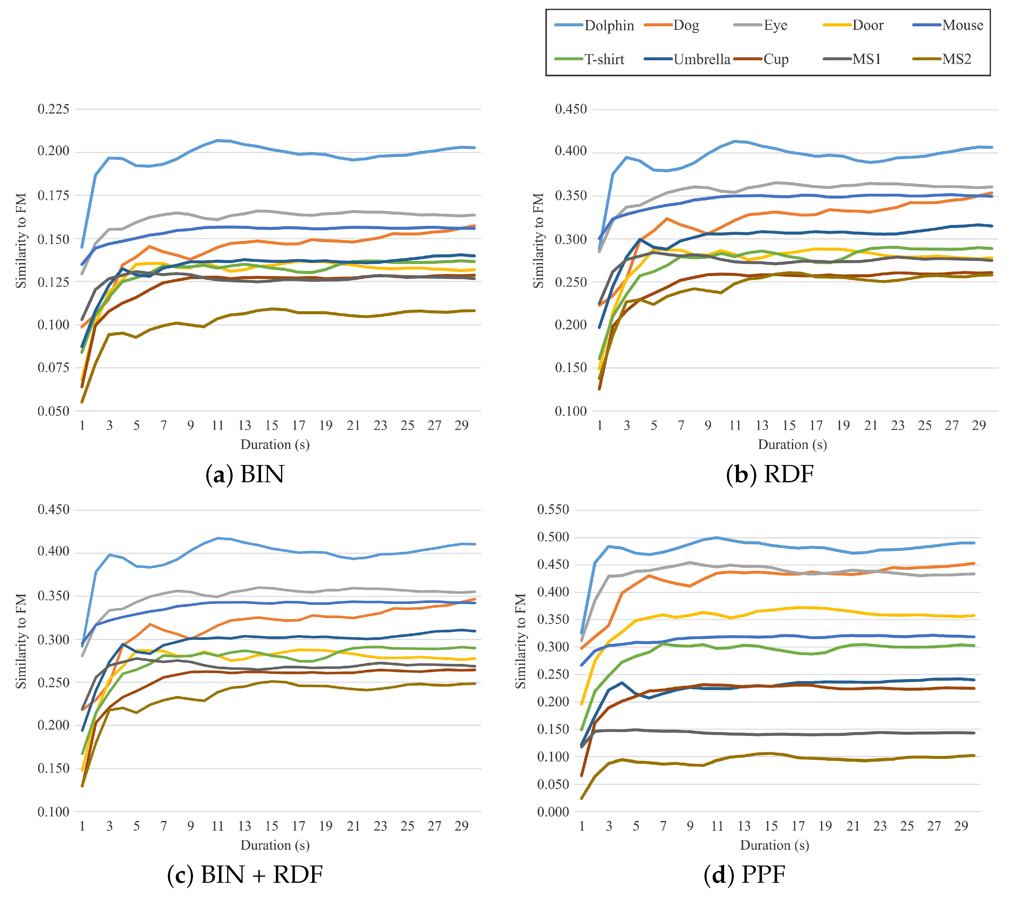
| Dolphin | Dog | Eye | Door | Mouse | T-Shirt | Umbrella | Cup | MS1 | MS2 | |
|---|---|---|---|---|---|---|---|---|---|---|
| BIN | 0.203 | 0.157 | 0.164 | 0.132 | 0.156 | 0.137 | 0.140 | 0.129 | 0.127 | 0.108 |
| RDF | 0.407 | 0.354 | 0.361 | 0.278 | 0.350 | 0.289 | 0.315 | 0.261 | 0.275 | 0.258 |
| BIN + RDF | 0.411 | 0.347 | 0.356 | 0.278 | 0.343 | 0.290 | 0.310 | 0.265 | 0.269 | 0.249 |
| PPF | 0.490 | 0.453 | 0.434 | 0.358 | 0.319 | 0.303 | 0.240 | 0.225 | 0.143 | 0.102 |
Publisher’s Note: MDPI stays neutral with regard to jurisdictional claims in published maps and institutional affiliations. |
© 2022 by the authors. Licensee MDPI, Basel, Switzerland. This article is an open access article distributed under the terms and conditions of the Creative Commons Attribution (CC BY) license (https://creativecommons.org/licenses/by/4.0/).
Share and Cite
Awano, N.; Hayashi, Y. Object Categorization Capability of Psychological Potential Field in Perceptual Assessment Using Line-Drawing Images. J. Imaging 2022, 8, 90. https://doi.org/10.3390/jimaging8040090
Awano N, Hayashi Y. Object Categorization Capability of Psychological Potential Field in Perceptual Assessment Using Line-Drawing Images. Journal of Imaging. 2022; 8(4):90. https://doi.org/10.3390/jimaging8040090
Chicago/Turabian StyleAwano, Naoyuki, and Yuki Hayashi. 2022. "Object Categorization Capability of Psychological Potential Field in Perceptual Assessment Using Line-Drawing Images" Journal of Imaging 8, no. 4: 90. https://doi.org/10.3390/jimaging8040090
APA StyleAwano, N., & Hayashi, Y. (2022). Object Categorization Capability of Psychological Potential Field in Perceptual Assessment Using Line-Drawing Images. Journal of Imaging, 8(4), 90. https://doi.org/10.3390/jimaging8040090