
Kidney Tumor Semantic Segmentation Using Deep Learning: A Survey of State-of-the-Art


Abstract
1. Introduction
2. Related Work
2.1. One-Stage Methods
2.2. Two-Stage Methods
2.3. Hybrid Models
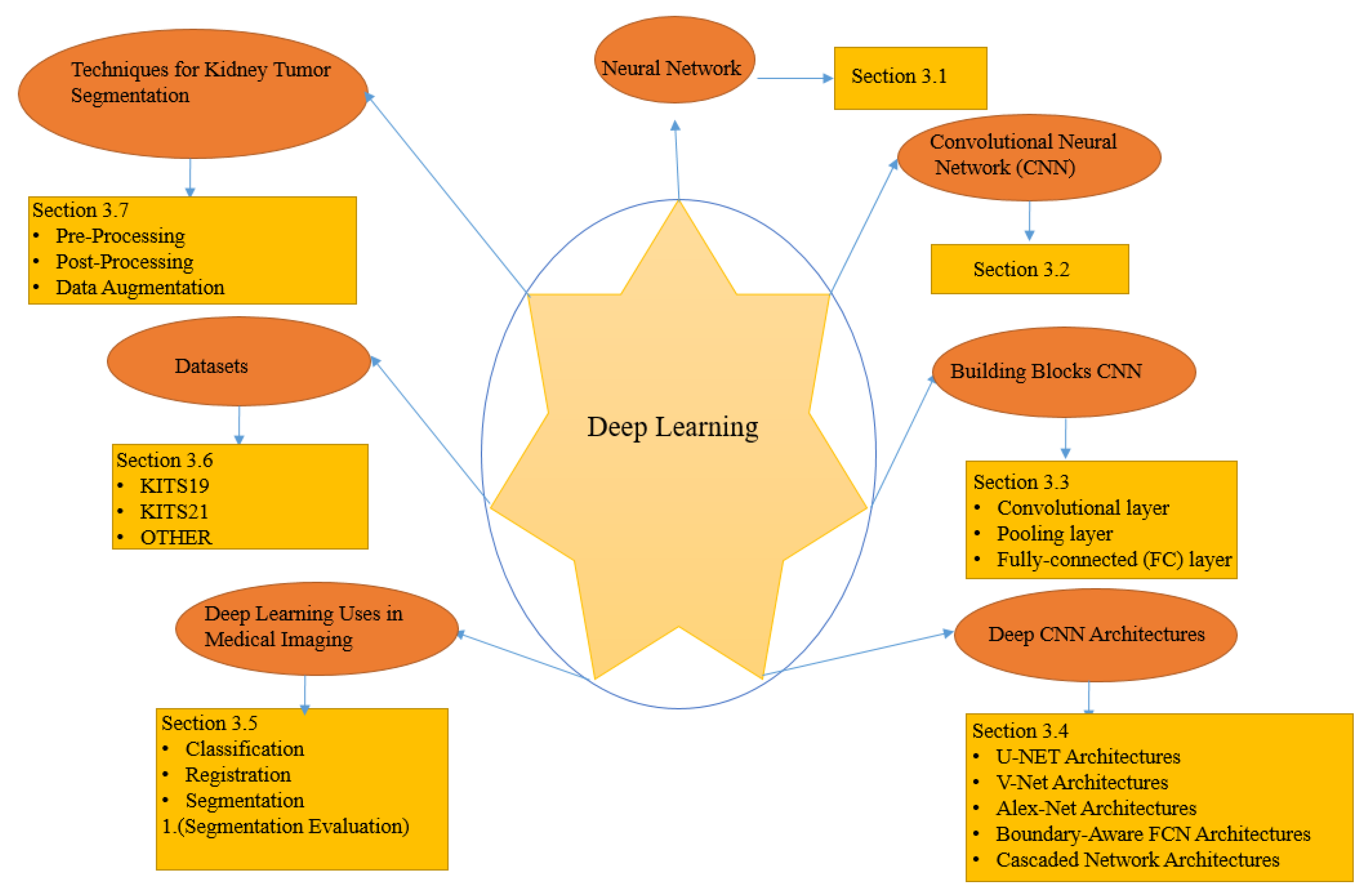
3. Overview of Deep Learning (DL) Models
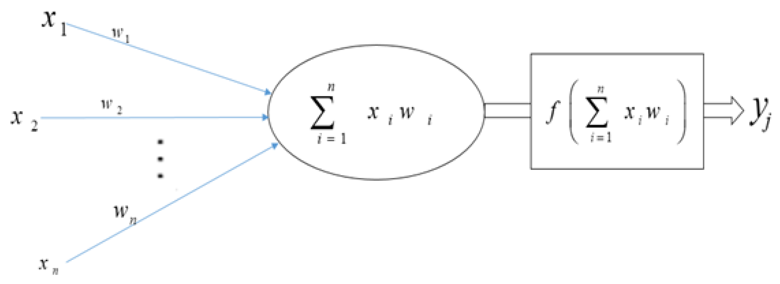
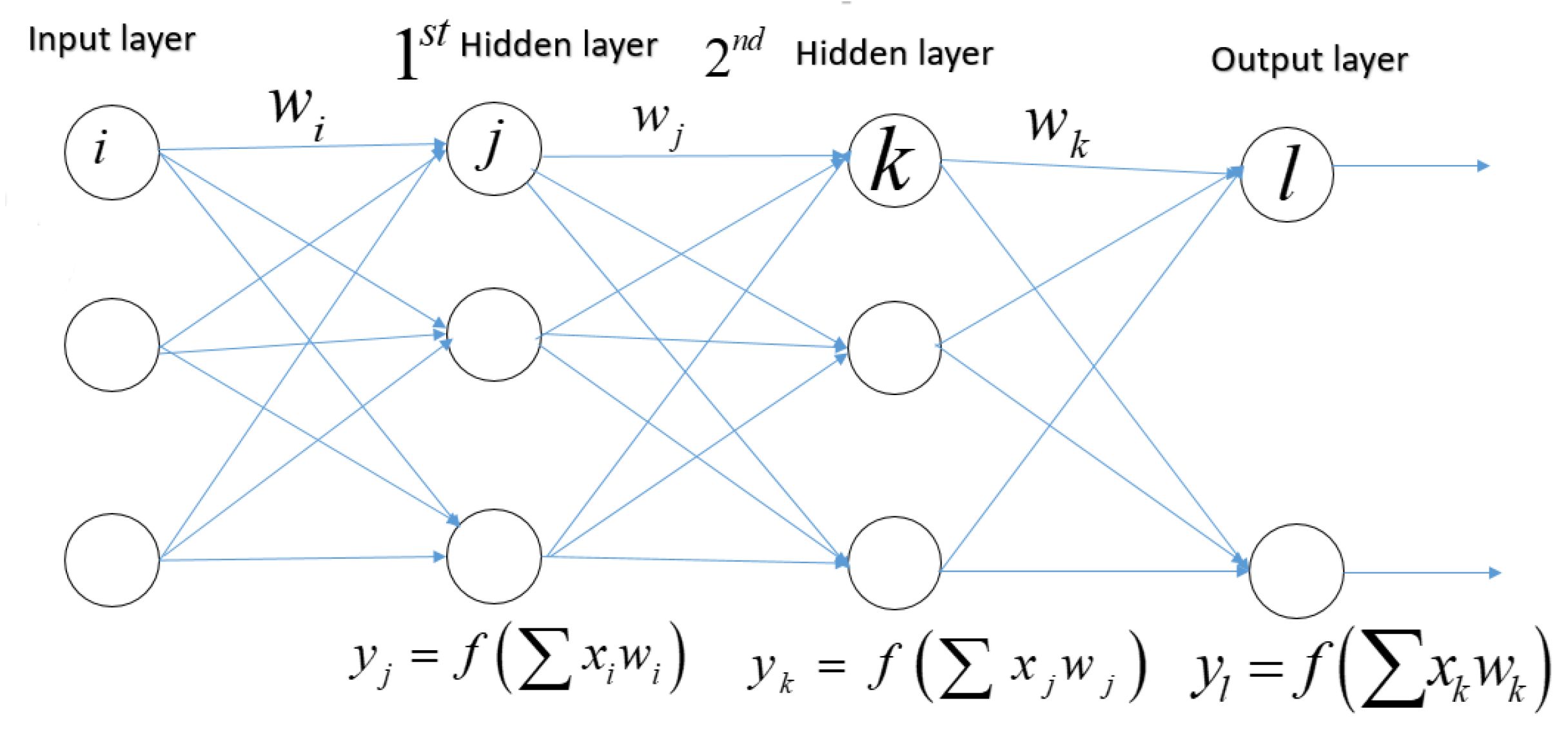
3.1. Neural Networks
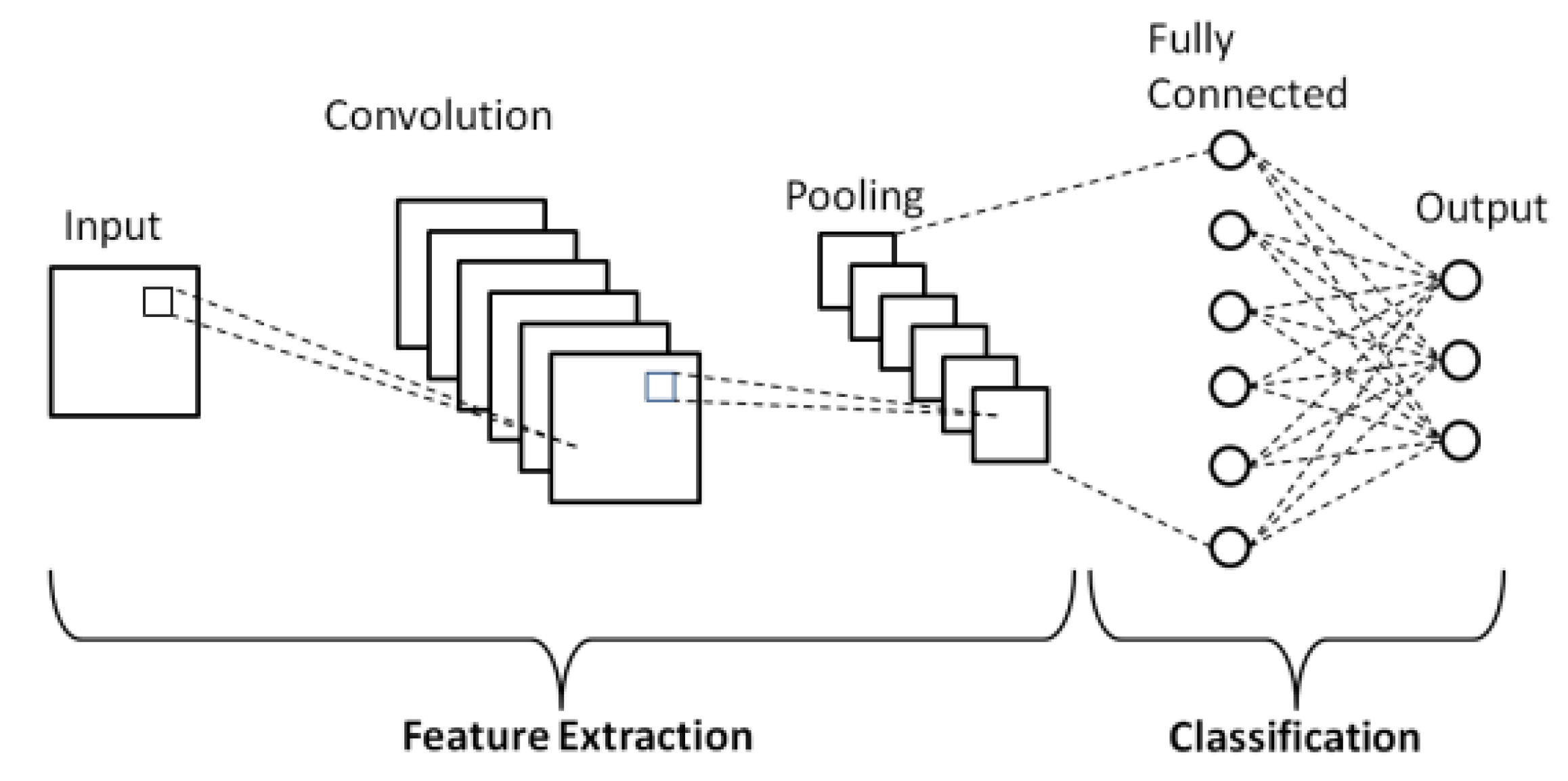
3.2. Convolutional Neural Network (CNN)
3.3. Building Blocks CNN
- Convolutional layer.
- Pooling layer.
- Fully-connected (FC) layer.
3.3.1. Convolutional Layer
3.3.2. Pooling Layer
3.3.3. Fully Connected (FC) Layer
3.4. Deep CNN Architectures
3.4.1. U-NET Architectures
3.4.2. V-Net Architectures
3.4.3. Alex-Net Architectures
3.4.4. Boundary-Aware FCN Architectures
3.4.5. Cascaded Network Architectures
3.5. Deep Learning Uses in Medical Imaging
3.5.1. Classification
3.5.2. Registration
3.5.3. Segmentation
3.5.4. Segmentation Evaluation
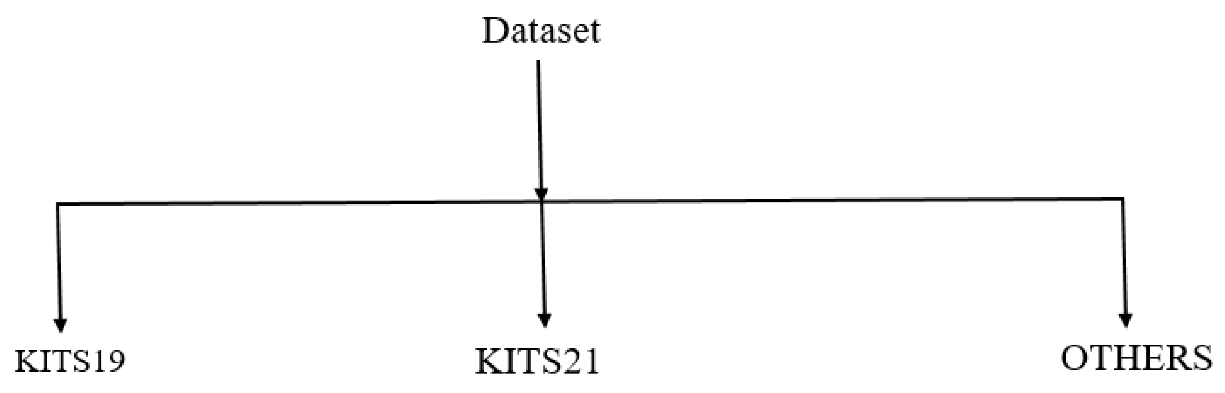
3.6. Datasets
3.7. Techniques for Kidney Tumor Segmentation
3.7.1. Pre-Processing
3.7.2. Post-Processing
3.7.3. Data Augmentation
4. Overview of Kidney Tumor Semantic Segmentation
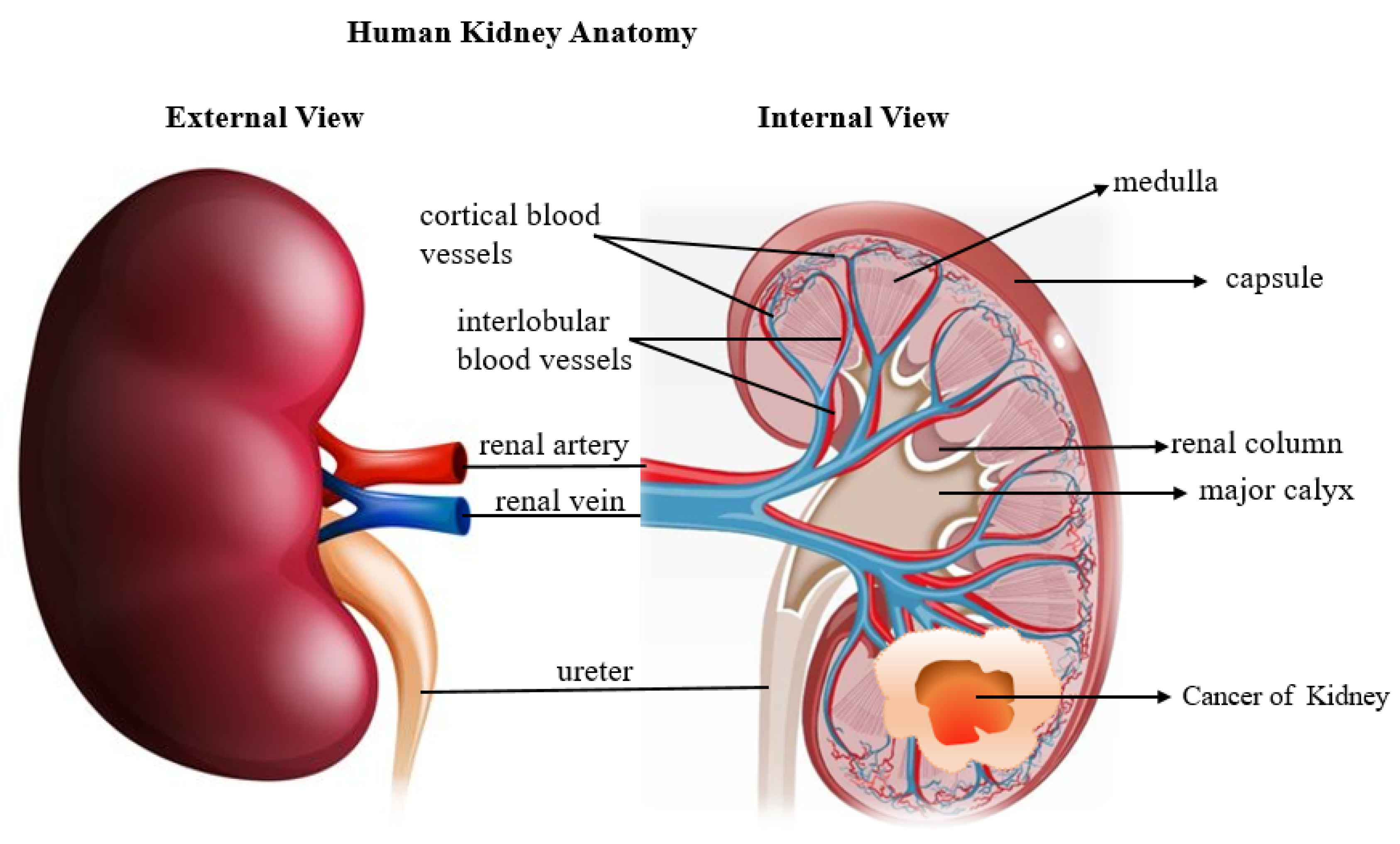
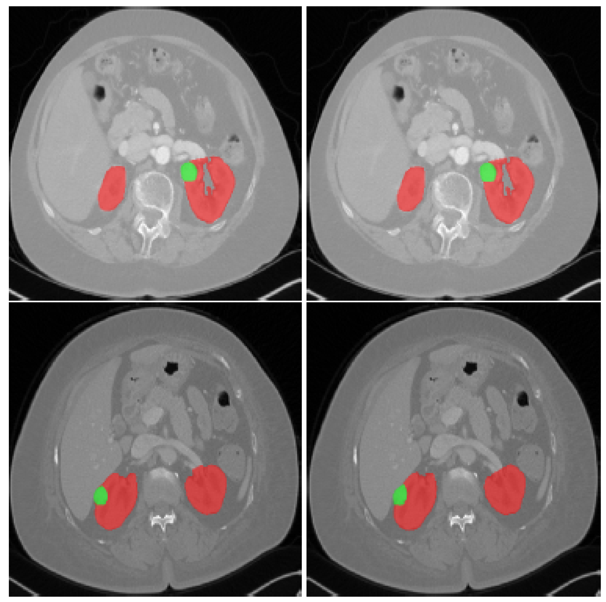
4.1. Renal Imaging
4.2. Image Segmentation
- The size of the image array where
- S and M represent the number of rows and columns.
4.3. Types of Segmentation
4.3.1. Manual Segmentation
4.3.2. Semi-Automatic Segmentation/Interactive Segmentation
4.3.3. Fully Automatic Segmentation
4.3.4. Semantic Segmentation
4.3.5. Semantic Segmentation Metrics
- Pixel accuracy can be computed as:
- Mean intersection over union can be computed as:
- Mean per class accuracy can be computed as:
5. Discussion
5.1. Kidney Tumor
5.2. Deep Learning
6. Conclusions and Future Work
Author Contributions
Funding
Institutional Review Board Statement
Informed Consent Statement
Data Availability Statement
Conflicts of Interest
References
- Kaur, R.; Juneja, M. A Survey of Kidney Segmentation Techniques in CT Images. Curr. Med. Imaging Rev. 2017, 14, 238–250. [Google Scholar] [CrossRef]
- Chen, X.; Summers, R.M.; Yao, J. Kidney Tumor Growth Prediction by Coupling Reaction-Diffusion and Biomechanical Model. IEEE Trans. Biomed. Eng. 2013, 60, 169–173. [Google Scholar] [CrossRef] [PubMed]
- Du, Z.; Chen, W.; Xia, Q.; Shi, O.; Chen, Q. Trends and Projections of Kidney Cancer Incidence at the Global and National Levels, 1990-2030: A Bayesian Age-Period-Cohort Modeling Study. Biomark. Res. 2020, 8, 1–10. [Google Scholar] [CrossRef] [PubMed]
- Smith, C.F.; Harvey, L.; Mills, K.; Harrison, H.; Rossi, S.H.; Griffin, S.J.; Stewart, G.D.; Usher, J.A. Reasons for Intending to Accept or Decline Kidney Cancer Screening: Thematic Analysis of Free Text from an Online Survey. BMJ Open 2021, 1–12. [Google Scholar] [CrossRef]
- Myronenko, A.; Hatamizadeh, A. 3D Kidneys and Kidney Tumor Semantic Segmentation Using Boundary-Aware Networks. arXiv 2019, arXiv:1909.06684. [Google Scholar]
- Heller, N.; Sathianathen, N.; Kalapara, A.; Walczak, E.; Moore, K.; Kaluzniak, H.; Rosenberg, J.; Blake, P.; Rengel, Z.; Oestreich, M.; et al. The KiTS19 Challenge Data: 300 Kidney Tumor Cases with Clinical Context, CT Semantic Segmentations, and Surgical Outcomes. arXiv 2019, arXiv:1904.00445. [Google Scholar]
- Greef, B.; Eisen, T. Medical Treatment of Renal Cancer: New Horizons. Br. J. Cancer 2016, 115, 505–516. [Google Scholar] [CrossRef]
- Hua, X.; Shi, H.; Zhang, L.; Xiao, H.; Liang, C. Systematic Analyses of The Role of Prognostic And Immunological of EIF3A, A Reader Protein, in Clear Cell Renal Cell Carcinoma. Cancer Cell Int. 2021, 21, 118. [Google Scholar]
- Millet, I.; Doyon, F.C.; Hoa, D.; Thuret, R.; Merigeaud, S.; Serre, I.; Taourel, P. Characterization of Small Solid Renal Lesions: Can Benign and Malignant Tumors Be Differentiated with CT? Am. J. Roentgenol. 2011, 197, 887–896. [Google Scholar] [CrossRef]
- Chawla, S.N.; Crispen, P.L.; Hanlon, A.L.; Greenberg, R.E.; Chen, D.Y.T.; Uzzo, R.G. The Natural History of Observed Enhancing Renal Masses: Meta-Analysis and Review of the World Literature. J. Urol. 2006, 175, 425–431. [Google Scholar] [CrossRef]
- Xie, Y.; Ma, X.; Li, H.; Gao, Y.; Gu, L.; Chen, L.; Zhang, X. Prognostic Value of Clinical and Pathological Features in Chinese Patients with Chromophobe Renal Cell Carcinoma: A 10-Year Single-Center Study. J. Cancer 2017, 8, 3474. [Google Scholar] [CrossRef] [PubMed]
- Zhao, W.; Jiang, D.; Peña Queralta, J.; Westerlund, T. MSS U-Net: 3D Segmentation of Kidneys and Tumors from CT Images with a Multi-Scale Supervised U-Net. Inform. Med. Unlocked 2020, 19, 100357. [Google Scholar] [CrossRef]
- Pan, X.; Quan, J.; Li, Z.; Zhao, L.; Zhou, L.; Jinling, X.; Weijie, X.; Guan, X.; Li, H.; Yang, S.; et al. MiR-566 Functions as an Oncogene and a Potential Biomarker for Prognosis in Renal Cell Carcinoma. Biomed. Pharmacother. 2018, 102, 718–727. [Google Scholar] [CrossRef]
- Hollingsworth, J.M.; Miller, D.C.; Daignault, S.; Hollenbeck, B.K. Rising Incidence of Small Renal Masses: A Need to Reassess Treatment Effect. J. Natl. Cancer Inst. 2006, 98, 1331–1334. [Google Scholar] [CrossRef] [PubMed]
- Cairns, P. Renal Cell Carcinoma. Cancer Biomark. 2011, 9, 461–473. [Google Scholar] [CrossRef] [PubMed]
- McLaughlin, J.K. Epidemiologic Characteristics and Risk Factors for Renal Cell Cancer. Clin. Epidemiol. 2009, 1, 33. [Google Scholar] [CrossRef] [PubMed]
- Sun, M.; Abdollah, F.; Bianchi, M.; Trinh, Q.D.; Jeldres, C.; Thuret, R.; Tian, Z.; Shariat, S.F.; Montorsi, F.; Perrotte, P.; et al. Treatment Management of Small Renal Masses in the 21st Century: A Paradigm Shift. Ann. Surg. Oncol. 2012, 19, 2380–2387. [Google Scholar] [CrossRef]
- Journal, P. Noise Issues Prevailing in Various Types of Medical Images. Biomed. Pharmacol. J. 2018, 11, 1227–1237. [Google Scholar]
- Mu, G.; Lin, Z.; Han, M.; Yao, G.; Gao, Y. Segmentation of Kidney Tumor by Multi-Resolution VB-Nets. Univ. Minn. Libr. 2019, 1–5. [Google Scholar] [CrossRef]
- Jung, I.K.; Jeong, Y.C.; Kyung, C.M.; Hak, J.L.; Seung, H.K. Segmental Enhancement Inversion at Biphasic Multidetector CT: Characteristic Finding of Small Renal Oncocytoma. Radiology 2009, 252, 441–448. [Google Scholar] [CrossRef]
- Magadza, T.; Viriri, S. Deep Learning for Brain Tumor Segmentation: A Survey of State-of-the-Art. J. Imaging 2021, 7, 19. [Google Scholar] [CrossRef] [PubMed]
- Dass, R.; Devi, S. Image Segmentation Techniques. Comput. Vis. Graph. Image Process. 2012, 7109, 66–70. [Google Scholar]
- Lateef, F.; Ruichek, Y. Survey on Semantic Segmentation Using Deep Learning Techniques. Neurocomputing 2019, 338, 321–348. [Google Scholar] [CrossRef]
- Xu, W.; Li, B.; Liu, S.; Qiu, W. Real-Time Object Detection and Semantic Segmentation for Autonomous Driving. MIPPR 2018, 2020, 44. [Google Scholar] [CrossRef]
- Tseng, Y.H.; Jan, S.S. Combination of Computer Vision Detection and Segmentation for Autonomous Driving. IEEE/ION Position Locat. Navig. Symp. Plans 2018, 1047–1052. [Google Scholar] [CrossRef]
- Jiang, F.; Grigorev, A.; Rho, S.; Tian, Z.; Fu, Y.S.; Jifara, W.; Adil, K.; Liu, S. Medical Image Semantic Segmentation Based on Deep Learning. Neural Comput. Appl. 2018, 29, 1257–1265. [Google Scholar] [CrossRef]
- Litjens, G.; Kooi, T.; Bejnordi, B.E.; Setio, A.A.A.; Ciompi, F.; Ghafoorian, M.; van der Laak, J.A.W.M.; van Ginneken, B.; Sánchez, C.I. A Survey on Deep Learning in Medical Image Analysis. Med. Image Anal. 2017, 42, 60–88. [Google Scholar] [CrossRef]
- Hesamian, M.H.; Jia, W.; He, X.; Kennedy, P. Deep Learning Techniques for Medical Image Segmentation: Achievements and Challenges. J. Digit. Imaging 2019, 32, 582–596. [Google Scholar] [CrossRef]
- Liu, H.; Lang, B. Machine Learning and Deep Learning Methods for Intrusion Detection Systems: A Survey. Appl. Sci. 2019, 9, 4396. [Google Scholar] [CrossRef]
- Hatamizadeh, A.; Hosseini, H.; Liu, Z.; Schwartz, S.D.; Terzopoulos, D. Deep Dilated Convolutional Nets for the Automatic Segmentation of Retinal Vessels. arXiv 2019, arXiv:1905.12120. [Google Scholar]
- Hatamizadeh, A.; Hoogi, A.; Sengupta, D.; Lu, W.; Wilcox, B.; Rubin, D.; Terzopoulos, D. Deep Active Lesion Segmentation. Lect. Notes Comput. Sci. 2019, 11861, 98–105. [Google Scholar] [CrossRef]
- Milletari, F.; Navab, N.; Ahmadi, S.A. V-Net: Fully Convolutional Neural Networks for Volumetric Medical Image Segmentation. Int. Conf. 3D Vision 2016, 2016, 565–571. [Google Scholar] [CrossRef]
- Lo, S.-C.B.; Lou, S.-L.A.; Lin, J.-S.; Freedman, M.T.; Chien, M.V.; Mun, S.K. And Applications for Lung Nodule Detection. IEEE Trans. Med. Imaging 1995, 14, 711–718. [Google Scholar] [CrossRef] [PubMed]
- Christ, P.F.; Ettlinger, F.; Grün, F.; Elshaera, M.E.A.; Lipkova, J.; Schlecht, S.; Ahmaddy, F.; Tatavarty, S.; Bickel, M.; Bilic, P.; et al. Automatic Liver and Tumor Segmentation of CT and MRI Volumes Using Cascaded Fully Convolutional Neural Networks. arXiv 2017, arXiv:1702.05970. [Google Scholar]
- Lin, T.Y.; Dollár, P.; Girshick, R.; He, K.; Hariharan, B.; Belongie, S. Feature Pyramid Networks for Object Detection. In Proceedings of the 2017 IEEE Conference on Computer Vision and Pattern Recognition (CVPR), Honolulu, HI, USA, 21–26 July 2017; pp. 936–944. [Google Scholar] [CrossRef]
- Zhao, H.; Shi, J.; Qi, X.; Wang, X.; Jia, J. Pyramid Scene Parsing Network. In Proceedings of the IEEE Conference on Computer Vision and Pattern Recognition (CVPR), Honolulu, HI, USA, 21–26 July 2017; pp. 6230–6239. [Google Scholar] [CrossRef]
- Doll, P.; Girshick, R.; Ai, F. Mask R-CNN. In Proceedings of the IEEE International Conference on Computer Vision (ICCV), Venice, Italy, 22–29 October 2017. [Google Scholar]
- Guo, Y.; Liu, Y.; Georgiou, T.; Lew, M.S. A Review of Semantic Segmentation Using Deep Neural Networks. Int. J. Multimed. Inf. Retr. 2018, 7, 87–93. [Google Scholar] [CrossRef]
- Isensee, F.; Maier-Hein, K.H. An Attempt at Beating the 3D U-Net. arXiv 2019, arXiv:1908.02182. [Google Scholar]
- Türk, F.; Lüy, M.; Barışçı, N. Kidney and Renal Tumor Segmentation Using a Hybrid V-Net-Based Model. Mathematics 2020, 8, 1772. [Google Scholar] [CrossRef]
- Xie, X.; Li, L.; Lian, S.; Chen, S.; Luo, Z. SERU: A Cascaded SE-ResNeXT U-Net for Kidney and Tumor Segmentation. Concurr. Comput. Pract. Exp. 2020, 32, 1–11. [Google Scholar] [CrossRef]
- Ali, A.M.; Farag, A.A.; El-Baz, A.S. Graph Cuts Framework for Kidney Segmentation with Prior Shape Constraints. Lect. Notes Comput. Sci. 2007, 4791, 384–392. [Google Scholar] [CrossRef]
- Thong, W.; Kadoury, S.; Piché, N.; Pal, C.J. Convolutional Networks for Kidney Segmentation in Contrast-Enhanced CT Scans. Comput. Methods Biomech. Biomed. Eng. Imaging Vis. 2018, 6, 277–282. [Google Scholar] [CrossRef]
- Myronenko, A.; Hatamizadeh, A. Edge-Aware Network for Kidneys and Kidney Tumor Semantic Segmentation; University of Minnesota Libraries Publishing: Mankato, MN, USA, 2019. [Google Scholar]
- Efremova, D.B.; Konovalov, D.A.; Siriapisith, T.; Kusakunniran, W.; Haddawy, P. Automatic Segmentation of Kidney and Liver Tumors in CT Images. arXiv 2019, arXiv:1908.01279. [Google Scholar] [CrossRef]
- Guo, J.; Zeng, W.; Yu, S.; Xiao, J. RAU-Net: U-Net Model Based on Residual and Attention for Kidney and Kidney Tumor Segmentation. In Proceedings of the 2021 IEEE International Conference on Consumer Electronics and Computer Engineering (ICCECE), Guangzhou, China, 15–17 January 2021; pp. 353–356. [Google Scholar] [CrossRef]
- Causey, J.; Stubblefield, J.; Qualls, J.; Fowler, J.; Cai, L.; Walker, K.; Guan, Y.; Huang, X. An Ensemble of U-Net Models for Kidney Tumor Segmentation with CT Images. IEEE/ACM Trans. Comput. Biol. Bioinforma. 2021, 5963, 1–5. [Google Scholar] [CrossRef]
- Nazari, M.; Jiménez-Franco, L.D.; Schroeder, M.; Kluge, A.; Bronzel, M.; Kimiaei, S. Automated and Robust Organ Segmentation for 3D-Based Internal Dose Calculation. EJNMMI Res. 2021, 11, 1–13. [Google Scholar] [CrossRef]
- George, Y. A Coarse-to-Fine 3D U-Net Network for Semantic Segmentation of Kidney CT Scans. Available online: https://openreview.net/forum?id=dvZiPuZk-Bc (accessed on 10 October 2021).
- Ruan, Y.; Li, D.; Marshall, H.; Miao, T.; Cossetto, T.; Chan, I.; Daher, O.; Accorsi, F.; Goela, A.; Li, S. MB-FSGAN: Joint Segmentation and Quantification of Kidney Tumor on CT by the Multi-Branch Feature Sharing Generative Adversarial Network. Med. Image Anal. 2020, 64, 101721. [Google Scholar] [CrossRef]
- Yu, Q.; Shi, Y.; Sun, J.; Gao, Y.; Zhu, J.; Dai, Y. Crossbar-Net: A Novel Convolutional Neural Network for Kidney Tumor Segmentation in CT Images. IEEE Trans. Image Process. 2019, 28, 4060–4074. [Google Scholar] [CrossRef] [PubMed]
- Pang, S.; Du, A.; Orgun, M.A.; Yu, Z.; Wang, Y.; Wang, Y.; Liu, G. CTumorGAN: A Unified Framework for Automatic Computed Tomography Tumor Segmentation. Eur. J. Nucl. Med. Mol. Imaging 2020, 47, 2248–2268. [Google Scholar] [CrossRef] [PubMed]
- Shen, Z.; Yang, H.; Zhang, Z.; Zheng, S. Automated Kidney Tumor Segmentation with Convolution and Transformer Network. Available online: https://openreview.net/forum?id=voteINyy36u (accessed on 10 October 2021).
- Yang, G.; Li, G.; Pan, T.; Kong, Y. Automatic Segmentation of Kidney and Renal Tumor in CT Images Based on 3D Fully Convolutional Neural Network with Pyramid Pooling Module. Int. Conf. Pattern Recognit. 2018, 31571001, 3790–3795. [Google Scholar] [CrossRef]
- Heo, J. Automatic Segmentation in Abdominal CT Imaging for the KiTS21 Challenge. Available online: https://openreview.net/forum?id=n6DR2TdGLa (accessed on 20 October 2021).
- Lund, C.B.; van der Velden, B.H.M. Leveraging Clinical Characteristics for Improved Deep Learning-Based Kidney Tumor Segmentation on CT. arXiv 2021, arXiv:2109.05816. [Google Scholar]
- Lin, C.; Fu, R.; Zheng, S. Kidney and Kidney Tumor Segmentation Using a Two-Stage Cascade Framework. Available online: https://openreview.net/forum?id=TDOSVEQ8mdO (accessed on 20 October 2021).
- da Cruz, L.B.; Araújo, J.D.L.; Ferreira, J.L.; Diniz, J.O.B.; Silva, A.C.; de Almeida, J.D.S.; de Paiva, A.C.; Gattass, M. Kidney Segmentation from Computed Tomography Images Using Deep Neural Network. Comput. Biol. Med. 2020, 123, 103906. [Google Scholar] [CrossRef]
- Zhang, Y.; Wang, Y.; Hou, F.; Yang, J.; Xiong, G.; Tian, J.; Zhong, C. Cascaded Volumetric Convolutional Network for Kidney Tumor Segmentation from CT Volumes. arXiv 2019, arXiv:1910.02235. [Google Scholar] [CrossRef]
- Hou, X.; Xie, C.; Li, F.; Wang, J.; Lv, C.; Xie, G.; Nan, Y. A Triple-Stage Self-Guided Network for Kidney Tumor Segmentation. In Proceedings of the 2020 IEEE 17th International Symposium on Biomedical Imaging (ISBI), Iowa City, IA, USA, 3–7 April 2020; pp. 341–344. [Google Scholar] [CrossRef]
- Hatamizadeh, A.; Terzopoulos, D.; Myronenko, A. Edge-Gated CNNs for Volumetric Semantic Segmentation of Medical Images. arXiv 2020, arXiv:2002.04207. [Google Scholar] [CrossRef]
- Santini, G.; Moreau, N.; Rubeaux, M. Kidney Tumor Segmentation Using an Ensembling Multi-Stage Deep Learning Approach. A Contribution to the KiTS19 Challenge. arXiv 2019, arXiv:1909.00735. [Google Scholar] [CrossRef]
- Chen, Z.; Liu, H. 2.5D Cascaded Semantic Segmentation for Kidney Tumor Cyst. Available online: https://openreview.net/forum?id=d5WM4_asJCl (accessed on 20 October 2021).
- Wei, H.; Wang, Q.; Zhao, W. Two-Phase Framework for Automatic Kidney and Kidney Tumor Segmentation. Available online: https://kits.lib.umn.edu/two-phase-framework-for-automatic-kidney-and-kidney-tumor-segmentation/ (accessed on 15 October 2021).
- He, T.; Zhang, Z.; Pei, C.; Huang, L. A Two-Stage Cascaded Deep Neural Network with Multi-Decoding Paths for Kidney Tumor Segmentation. Available online: https://openreview.net/forum?id=c7kCK-E-B1 (accessed on 10 October 2021).
- Lv, Y.; Wang, J. Three Uses of One Neural Network: Automatic Segmentation of Kidney Tumor and Cysts Based on 3D U-Net. Available online: https://openreview.net/forum?id=UzoGQ8fO_8f (accessed on 15 October 2021).
- Li, D.; Chen, Z.; Hassan, H.; Xie, W.; Huang, B. A Cascaded 3D Segmentation Model for Renal Enhanced CT Images. Available online: https://openreview.net/forum?id=dKvuhx2UPO3 (accessed on 10 October 2021).
- Xiao, C.; Hassan, H.; Huang, B. Contrast-Enhanced CT Renal Tumor Segmentation. Available online: https://openreview.net/forum?id=-QutS3TdRu- (accessed on 20 October 2021).
- Wen, J.; Li, Z.; Shen, Z.; Zheng, Y. Squeeze-and-Excitation Encoder-Decoder Network for Kidney and Kidney Tumor Segmentation in CT Images. Available online: https://openreview.net/forum?id=uC-Gl3IG8wn (accessed on 10 October 2021).
- Qayyum, A.; Lalande, A.; Meriaudeau, F. Automatic Segmentation of Tumors and Affected Organs in the Abdomen Using a 3D Hybrid Model for Computed Tomography Imaging. Comput. Biol. Med. 2020, 127, 104097. [Google Scholar] [CrossRef] [PubMed]
- Cheng, J.; Liu, J.; Liu, L.; Pan, Y.; Wang, J. A Double Cascaded Framework Based on 3D SEAU-Net for Kidney and Kidney Tumor Segmentation; University of Minnesota Libraries Publishing: Mankato, MN, USA, 2019; pp. 1–6. [Google Scholar]
- da Cruz, L.B.; Júnior, D.A.D.; Diniz, J.O.B.; Silva, A.C.; de Almeida, J.D.S.; de Paiva, A.C.; Gattass, M. Kidney Tumor Segmentation from Computed Tomography Images Using DeepLabv3+ 2.5D Model. Expert Syst. Appl. 2021, 192, 116270. [Google Scholar] [CrossRef]
- Zhao, W.; Zeng, Z. Multi Scale Supervised 3D U-Net for Kidney and Tumor Segmentation. arXiv 2019, arXiv:1908.03204. [Google Scholar] [CrossRef]
- Meyer, J.G. Deep Learning Neural Network Tools for Proteomics. Cell Rep. Methods 2021, 1, 100003. [Google Scholar] [CrossRef]
- Fukushima, K. Neocognitron: A Self-Organizing Neural Network Model for a Mechanism of Pattern Recognition Unaffected by Shift in Position. Biol. Cybern. 1980, 36, 193–202. [Google Scholar] [CrossRef]
- Baumgartl, H.; Tomas, J.; Buettner, R.; Merkel, M. A Deep Learning-Based Model for Defect Detection in Laser-Powder Bed Fusion Using in-Situ Thermographic Monitoring. Prog. Addit. Manuf. 2020, 5, 277–285. [Google Scholar] [CrossRef]
- Buettner, R.; Baumgartl, H. A Highly Effective Deep Learning Based Escape Route Recognition Module for Autonomous Robots in Crisis and Emergency Situations. Proc. Annu. Hawaii Int. Conf. Syst. Sci. 2019, 2019, 659–666. [Google Scholar] [CrossRef]
- Dalal, N.; Triggs, B. Histograms of Oriented Gradients for Human Detection. In Proceedings of the 2005 IEEE Computer Society Conference on Computer Vision and Pattern Recognition (CVPR’05), San Diego, CA, USA, 20–25 June 2005; pp. 886–893. [Google Scholar] [CrossRef]
- Bay, H.; Tuytelaars, T.; Van Gool, L. SURF: Speeded Up Robust Features. Comput. Vis. Image Underst. 2006, 110, 404–417. [Google Scholar]
- Fazl-Ersi, E.; Tsotsos, J.K. Histogram of Oriented Uniform Patterns for Robust Place Recognition and Categorization. Int. J. Rob. Res. 2012, 31, 468–483. [Google Scholar] [CrossRef]
- LeCun, Y.; Bottou, L.; Bengio, Y.; Haffner, P. Gradient-Based Learning Applied to Document Recognition. Proc. IEEE 1998, 86, 2278–2323. [Google Scholar] [CrossRef]
- Koushik, J. Understanding Convolutional Neural Networks. arXiv 2016, arXiv:1605.09081. [Google Scholar]
- Ronneberger, O.; Fischer, P.; Brox, T. U-Net: Convolutional Networks for Biomedical Image Segmentation BT-Medical Image Computing and Computer-Assisted Intervention–MICCAI 2015; Navab, N., Hornegger, J., Wells, W.M., Frangi, A.F., Eds.; Springer International Publishing: Berlin/Heidelberg, Germany, 2015; pp. 234–241. [Google Scholar]
- Štern, D.; Bischof, H.; Urschler, M. Regressing Heatmaps for Multiple Landmark Localization Using CNNs Automatic Age Estimation from Skeletal and Dental MRI Data Using Machine Learning View Project SEE PROFILE Regressing Heatmaps for Multiple Landmark Localization Using CNNs; Springer International Publishing: Berlin/Heidelberg, Germany, 2016. [Google Scholar]
- Mkrtchyan, K.; Singh, D.; Liu, M.; Reddy, V.; Roy-Chowdhury, A.; Gopi, M. Efficient Cell Segmentation and Tracking of Developing Plant Meristem. In Proceedings of the 2011 18th IEEE International Conference on Image Processing, Brussels, Belgium, 11–14 September 2011; pp. 2165–2168. [Google Scholar] [CrossRef]
- Chang, C.S.; Ding, J.J.; Chen, P.H.; Wu, Y.F.; Lin, S.J. 3-D Cell Segmentation by Improved V-Net Architecture Using Edge and Boundary Labels. In Proceedings of the 2019 IEEE 2nd International Conference on Information Communication and Signal Processing (ICICSP), Weihai, China, 28–30 September 2019; pp. 435–439. [Google Scholar] [CrossRef]
- Shanthi, T.; Sabeenian, R.S. Modified Alexnet Architecture for Classification of Diabetic Retinopathy Images. Comput. Electr. Eng. 2019, 76, 56–64. [Google Scholar] [CrossRef]
- Jiang, H.; Diao, Z.; Yao, Y.-D. Deep Learning Techniques for Tumor Segmentation: A Review. J. Supercomput. 2021. [Google Scholar] [CrossRef]
- Shen, H.; Wang, R.; Zhang, J.; McKenna, S.J. Boundary-Aware Fully Convolutional Network for Brain Tumor Segmentation. Lect. Notes Comput. Sci. 2017, 10434, 433–441. [Google Scholar] [CrossRef]
- Havaei, M.; Davy, A.; Warde-Farley, D.; Biard, A.; Courville, A.; Bengio, Y.; Pal, C.; Jodoin, P.M.; Larochelle, H. Brain Tumor Segmentation with Deep Neural Networks. Med. Image Anal. 2017, 35, 18–31. [Google Scholar] [CrossRef]
- Wang, G.; Li, W.; Ourselin, S.; Vercauteren, T. Automatic Brain Tumor Segmentation Based on Cascaded Convolutional Neural Networks with Uncertainty Estimation. Front. Comput. Neurosci. 2019, 13, 56. [Google Scholar] [CrossRef] [PubMed]
- Wang, Z.; Wang, E.; Zhu, Y. Image Segmentation Evaluation: A Survey of Methods; Springer: Berlin/Heidelberg, Germany, 2020; Volume 53. [Google Scholar] [CrossRef]
- Di Leo, G.; Di Terlizzi, F.; Flor, N.; Morganti, A.; Sardanelli, F. Measurement of Renal Volume Using Respiratory-Gated MRI in Subjects without Known Kidney Disease: Intraobserver, Interobserver, and Interstudy Reproducibility. Eur. J. Radiol. 2011, 80, e212–e216. [Google Scholar] [CrossRef] [PubMed]
- King, B.F.; Reed, J.E.; Bergstralh, E.J.; Sheedy, P.F.; Torres, V.E. Quantification and Longitudinal Trends of Kidney, Renal Cyst, and Renal Parenchyma Volumes in Autosomal Dominant Polycystic Kidney Disease. J. Am. Soc. Nephrol. 2000, 11, 1505–1511. [Google Scholar] [CrossRef] [PubMed]
- Taha, A.A.; Hanbury, A. Metrics for Evaluating 3D Medical Image Segmentation: Analysis, Selection, and Tool. BMC Med. Imaging 2015, 15, 1–28. [Google Scholar] [CrossRef] [PubMed]
- Dogra, D.P.; Majumdar, A.K.; Sural, S. Evaluation of Segmentation Techniques Using Region Area and Boundary Matching Information. J. Vis. Commun. Image Represent. 2012, 23, 150–160. [Google Scholar] [CrossRef]
- Karimi, D.; Salcudean, S.E. Reducing the Hausdorff Distance in Medical Image Segmentation with Convolutional Neural Networks. IEEE Trans. Med. Imaging 2020, 39, 499–513. [Google Scholar] [CrossRef] [PubMed]
- Kirasich, K.; Smith, T.; Sadler, B. Random Forest vs Logistic Regression: Binary Classification for Heterogeneous Datasets. Data Sci. Rev. 2018, 1, 9. [Google Scholar]
- Kaur, R.; Juneja, M.; Mandal, A.K. A Hybrid Edge-Based Technique for Segmentation of Renal Lesions in CT Images. Multimed. Tools Appl. 2019, 78, 12917–12937. [Google Scholar] [CrossRef]
- Dill, V.; Franco, A.R.; Pinho, M.S. Automated Methods for Hippocampus Segmentation: The Evolution and a Review of the State of the Art. Neuroinformatics 2015, 13, 133–150. [Google Scholar] [CrossRef]
- Yu, J.; Xu, J.; Chen, Y.; Li, W.; Wang, Q.; Yoo, B.; Han, J.-J. Learning Generalized Intersection Over Union for Dense Pixelwise Prediction. PMLR 2021, 139, 12198–12207. [Google Scholar]
- Wu, H.; Yang, S.; Huang, Z.; He, J.; Wang, X. Type 2 Diabetes Mellitus Prediction Model Based on Data Mining. Inform. Med. Unlocked 2018, 10, 100–107. [Google Scholar] [CrossRef]
- Saito, T.; Rehmsmeier, M. The Precision-Recall Plot Is More Informative than the ROC Plot When Evaluating Binary Classifiers on Imbalanced Datasets. PLoS ONE 2015, 10, e0118432. [Google Scholar] [CrossRef] [PubMed]
- Tahir, B.; Iqbal, S.; Usman Ghani Khan, M.; Saba, T.; Mehmood, Z.; Anjum, A.; Mahmood, T. Feature Enhancement Framework for Brain Tumor Segmentation and Classification. Microsc. Res. Tech. 2019, 82, 803–811. [Google Scholar] [CrossRef] [PubMed]
- Sled, J.G.; Zijdenbos, A.P.; Evans, A.C. A Nonparametric Method for Automatic Correction of Intensity Nonuniformity in Mri Data. IEEE Trans. Med. Imaging 1998, 17, 87–97. [Google Scholar] [CrossRef] [PubMed]
- Tustison, N.J.; Avants, B.B.; Cook, P.A.; Zheng, Y.; Egan, A.; Yushkevich, P.A.; Gee, J.C. N4ITK: Improved N3 Bias Correction. IEEE Trans. Med. Imaging 2010, 29, 1310–1320. [Google Scholar] [CrossRef]
- Nyúl, L.G.; Udupa, J.K.; Zhang, X. New Variants of a Method of MRI Scale Standardization. IEEE Trans. Med. Imaging 2000, 19, 143–150. [Google Scholar] [CrossRef] [PubMed]
- Kamnitsas, K.; Ledig, C.; Newcombe, V.F.J.; Simpson, J.P.; Kane, A.D.; Menon, D.K.; Rueckert, D.; Glocker, B. Efficient Multi-Scale 3D CNN with Fully Connected CRF for Accurate Brain Lesion Segmentation. Med. Image Anal. 2017, 36, 61–78. [Google Scholar] [CrossRef]
- Gordillo, N.; Montseny, E.; Sobrevilla, P. State of the Art Survey on MRI Brain Tumor Segmentation. Magn. Reson. Imaging 2013, 31, 1426–1438. [Google Scholar] [CrossRef]
- Dong, H.; Yang, G.; Liu, F.; Mo, Y.; Guo, Y. Automatic Brain Tumor Detection and Segmentation Using U-Net Based Fully Convolutional Networks. Commun. Comput. Inf. Sci. 2017, 723, 506–517. [Google Scholar] [CrossRef]
- Torres, H.R.; Queirós, S.; Morais, P.; Oliveira, B.; Fonseca, J.C.; Vilaça, J.L. Kidney Segmentation in Ultrasound, Magnetic Resonance and Computed Tomography Images: A Systematic Review. Comput. Methods Programs Biomed. 2018, 157, 49–67. [Google Scholar] [CrossRef]
- Udupa, J.K.; Leblanc, V.R.; Schmidt, H.; Imielinska, C.; Saha, P.K. A Methodology for Evaluating Image Segmentation Algorithms Medical Image Processing Group—Department of Radiology—University of Pennsylvania. Image Processing. Int. Soc. Opt. Photonics 2002, 4684, 266–277. [Google Scholar]
- Fasihi, M.S.; Mikhael, W.B. Overview of Current Biomedical Image Segmentation Methods. In Proceedings of the 2016 International Conference on Computational Science and Computational Intelligence (CSCI), Las Vegas, NV, USA, 15–17 December 2016; pp. 803–808. [Google Scholar] [CrossRef]
- Ramkumar, A.; Dolz, J.; Kirisli, H.A.; Adebahr, S.; Schimek-Jasch, T.; Nestle, U.; Massoptier, L.; Varga, E.; Stappers, P.J.; Niessen, W.J.; et al. User Interaction in Semi-Automatic Segmentation of Organs at Risk: A Case Study in Radiotherapy. J. Digit. Imaging 2016, 29, 264–277. [Google Scholar] [CrossRef] [PubMed]
- Bae, K.T.; Shim, H.; Tao, C.; Chang, S.; Wang, J.H.; Boudreau, R.; Kwoh, C.K. Intra- and Inter-Observer Reproducibility of Volume Measurement of Knee Cartilage Segmented from the OAI MR Image Set Using a Novel Semi-Automated Segmentation Method. Osteoarthr. Cartil. 2009, 17, 1589–1597. [Google Scholar] [CrossRef] [PubMed]
- Gaonkar, B.; Macyszyn, L.; Bilello, M.; Sadaghiani, M.S.; Akbari, H.; Atthiah, M.A.; Ali, Z.S.; Da, X.; Zhan, Y.; Rourke, D.O.; et al. Automated Tumor Volumetry Using Computer-Aided Image Segmentation. Acad. Radiol. 2015, 22, 653–661. [Google Scholar] [CrossRef]
- Graber, C.; Tsai, G.; Firman, M.; Brostow, G.; Schwing, A. Panoptic Segmentation Forecasting. arXiv 2021, arXiv:2104.03962. [Google Scholar]
- Thoma, M. A Survey of Semantic Segmentation. arXiv 2016, arXiv:1602.06541. [Google Scholar]
- Liu, X.; Deng, Z.; Yang, Y. Recent Progress in Semantic Image Segmentation. Artif. Intell. Rev. 2019, 52, 1089–1106. [Google Scholar] [CrossRef]
- Garcia-Garcia, A.; Orts-Escolano, S.; Oprea, S.; Villena-Martinez, V.; Garcia-Rodriguez, J. A Review on Deep Learning Techniques Applied to Semantic Segmentation. arXiv 2017, arXiv:1704.06857. [Google Scholar]
- Bou, A. Deep Learning Models for Semantic Segmentation of Mammography Screenings. 2019. Available online: https://www.diva-portal.org/smash/record.jsf?pid=diva2:1380578 (accessed on 10 October 2021).
- Menze, B.H.; Jakab, A.; Bauer, S.; Kalpathy-Cramer, J.; Farahani, K.; Kirby, J.; Burren, Y.; Porz, N.; Slotboom, J.; Wiest, R.; et al. The Multimodal Brain Tumor Image Segmentation Benchmark (BRATS). IEEE Trans. Med. Imaging 2015, 34, 1993–2024. [Google Scholar] [CrossRef]
- Arel, I.; Rose, D.; Karnowski, T. Deep Machine Learning-A New Frontier in Artificial Intelligence Research. IEEE Comput. Intell. Mag. 2010, 5, 13–18. [Google Scholar] [CrossRef]
- Krizhevsky, A.; Sutskever, I.; Hinton, G.E. ImageNet Classification with Deep Convolutional Neural Networks. Commun. ACM 2017, 60, 84–90. [Google Scholar] [CrossRef]
- Collobert, R.; Weston, J. A Unified Architecture for Natural Language Processing: Deep Neural Networks with Multitask Learning. In Proceedings of the 25th International Conference on Machine Learning, Helsinki, Finland, 5–9 July 2008; pp. 160–167. [Google Scholar] [CrossRef]
- Lee, H.; Yan, L.; Pham, P.; Ng, A.Y. Unsupervised Feature Learning for Audio Classification Using Convolutional Deep Belief Networks. Adv. Neural Inf. Process. Syst. Proc. 2009, 1096–1104. Available online: https://proceedings.neurips.cc/paper/2009/hash/a113c1ecd3cace2237256f4c712f61b5-Abstract.html (accessed on 10 October 2021).
- Graham-Knight, J.B.; Djavadifar, A.; Lasserre, D.P.; Najjaran, H. Applying NnU-Net to the KiTS19 Grand Challenge. Univ. Minn. Libr. 2019, 1–7. [Google Scholar] [CrossRef]
- Rao, P.K.; Chatterjee, S. WP-UNet: Weight Pruning U-Net with Depthwise Separable Convolutions for Semantic Segmentation of Kidney Tumors. ResearchSquare 2021. [Google Scholar] [CrossRef]
- Sabarinathan, D.; Parisa Beham, M.; Mansoor Roomi, S.M.M. Hyper Vision Net: Kidney Tumor Segmentation Using Coordinate Convolutional Layer and Attention Unit. Commun. Comput. Inf. Sci. 2020, 1249, 609–618. [Google Scholar] [CrossRef]
- Yuan, Y. Automatic Kidney and Tumor Segmentation with Hybrid Hierarchical Networks. Comput. Biol. Med. 2019. [Google Scholar] [CrossRef]
- Sharma, R.; Halarnkar, P.; Choudhari, K. Kidney and Tumor Segmentation Using U-Net Deep Learning Model. SSRN Electron. J. 2020, 2020. [Google Scholar] [CrossRef]
- Li, C.; Chen, W.; Tan, Y. Point-Samplingmethod Based on 3DU-Net Architecture to Reduce the Influence of False Positive and Solve Boundary Blur Problemin 3DCT Image Segmentation. Appl. Sci. 2020, 10, 6838. [Google Scholar] [CrossRef]
- Akram, Z. Cancerous Tumor Segmentation of Kidney Images and Prediction of Tumor Using Medical Image Segmentation and Deep Learning Techniques. Clin. Oncol. 2021, 4, 1–9. [Google Scholar]
- Daza, L.; Gómez, C.; Arbeláez, P. Semantic Segmentation of Kidney Tumor Using Convolutional Neural Networks. Univ. Minn. Libr. 2019. [Google Scholar] [CrossRef]
- Shen, C.; Wang, C.; Oda, M.; Mori, K. Coarse-to-Fine Kidney and Tumor Segmentation with Fully Convolutional Networks. arXiv 2019, arXiv:1908.11064v1. [Google Scholar] [CrossRef]
- Vu, M.H.; Grimbergen, G.; Simkó, A.; Nyholm, T.; Löfstedt, T. Localization Network and End-to-End Cascaded U-Nets for Kidney Tumor Segmentation. Univ. Minn. Libr. 2019. [Google Scholar] [CrossRef]
- Lv, Y.; Wang, J. Kidney Tumor Segmentation Based on U-Net and V-Net with Double Loss Function Training. Univ. Minn. Libr. 2019, 1–4. [Google Scholar] [CrossRef]
- Xia, K.; Yin, H.; Zhang, Y. Deep Semantic Segmentation of Kidney and Space-Occupying Lesion Area Based on SCNN and ResNet Models Combined with SIFT-Flow Algorithm. J. Med. Syst. 2019, 43, 1–12. [Google Scholar] [CrossRef]
- Bakas, S.; Reyes, M.; Jakab, A.; Bauer, S.; Rempfler, M.; Crimi, A.; Shinohara, R.T.; Berger, C.; Ha, S.M.; Rozycki, M.; et al. Identifying the Best Machine Learning Algorithms for Brain Tumor Segmentation, Progression Assessment, and Overall Survival Prediction in the BRATS Challenge. arXiv 2018, arXiv:1811.02629. [Google Scholar]
- Shorten, C.; Khoshgoftaar, T.M. A Survey on Image Data Augmentation for Deep Learning. J. Big Data 2019, 6, 1–48. [Google Scholar] [CrossRef]
- Pavlov, S.; Artemov, A.; Sharaev, M.; Bernstein, A.; Burnaev, E. Weakly Supervised Fine Tuning Approach for Brain Tumor Segmentation Problem. In Proceedings of the 2019 18th IEEE International Conference On Machine Learning and Applications (ICMLA), Boca Raton, FL, USA, 16–19 December 2019; pp. 1600–1605. [Google Scholar] [CrossRef]
- Sarker, I.H. Deep Learning: A Comprehensive Overview on Techniques, Taxonomy, Applications and Research Directions. SN Comput. Sci. 2021, 2, 1–20. [Google Scholar] [CrossRef]
- Zikic, D.; Ioannou, Y.; Brown, M.; Criminisi, A. Segmentation of Brain Tumor Tissues with Convolutional Neural Networks. Proc. MICCAI-BRATS 2014, 2014, 36–39. [Google Scholar]
- Wang, L.; Wang, S.; Chen, R.; Qu, X.; Chen, Y.; Huang, S.; Liu, C. Nested Dilation Networks for Brain Tumor Segmentation Based on Magnetic Resonance Imaging. Front. Neurosci. 2019, 13, 1–14. [Google Scholar] [CrossRef] [PubMed]


| Metric | Equation | Description |
|---|---|---|
| True Positive rate (TP) | = = = | True positive rate, the proportion of true positives or successes that is accurately detected, is calculated as true positive rate, also known as sensitivity [98]. |
| True Negative rate (TN) | = = = | The true negative rate, also known as specificity, is the true negative rate. Is there a the chance that a non-diseased will the person be classified as negative by the test? It demonstrates the test’s sensitivity in identifying the absence of illness [99]. |
| False-positive rate (FP) | = | The false-positive rate refers to the percentage of mistakenly classified as positive or successful but as negative [98]. |
| Dice Similarity Coefficient (DSC) | = 2× | The binary mask produced by the domain experts’ manual segmentation corresponds to the binary mask produced by the suggested approach. DC must be close to unity to guarantee that the manually drawn region corresponds to the segmented result correctly [99]. |
| Jaccard Index JI | = | The Jaccard Index (JI) was used to compare the statistical similarity of regions segmented using a computational approach to hand delineations [100,101]. |
| Accuracy | = | The correct predictions produced by the prediction model across all suitable forecasts completed are referred to as the model’s accuracy [102]. |
| Precision | = | The number of correct positive scores divided by the number of positive scores anticipated by the classification algorithm is the positive predictive value, or precision [103]. |
| Sørensen–Dice | = | This coefficient: Indicates the extent to which segmented and reference volumes overlap in mm3. (1 for ideal segmentation, 0 for the worst-case scenario) When applied to Boolean data, the terms true positive (TP), false positive (FP), and false negative (FN) are used (FN), As in this case [47]. |
| References | Total | Training Data | Validation | Testing Data |
|---|---|---|---|---|
| KITS19 [39,40,44,59,72] | 300 | 210 | - | 90 |
| KITS19 [12] | 210 | 134 | 34 | 42 |
| KITS19 [61] | 300 | 240 | - | 60 |
| KITS19 [62] | 300 | 190 | 20 | 90 |
| KITS19 [70] | 300 | 240 | 30 | 30 |
| KITS19 [41,58] | 300 | 168 | 42 | 90 |
| KITS21 [55,63,65,69] | 300 | 240 | - | 60 |
| OTHER [50] | 113 | 70 | 23 | 20 |
| OTHER [54] | 140 | 90 | - | 50 |
| Type of Segmentation | Reproducibility | Time | Interactivity | Complexity of Implementation |
|---|---|---|---|---|
| Manual Segmentation | Good | Too long | Bad | Easy |
| Semi-Automatic Segmentation | Good | Long | Not bad | Easy |
| Fully Automatic Segmentation | Good | Short | Good | Hard |
| Semantic Segmentation | Good | Short | Good | Hard |
| Reference | Input | Regulization | Activation | Loss | Optimizer |
|---|---|---|---|---|---|
| U-Net Architecture | |||||
| [127] | 3D | Dice | Decathalon | ||
| [128] | 3D | BN, Depthwise, Weight Pruning | RELU | Mean IoU, AC | Adam |
| [49] | 3D,2D | RELU | Dice | SGD | |
| [129] | 3D | Dice | Adam | ||
| [60] | 3D | Leaky ReLU | Dice | Adam | |
| [53] | 3D | Dice, SD | Adam | ||
| [12] | 3D | IN | Dice | Adam | |
| [130] | 3D,2D | BN | ReLU | Dice | Adam |
| [131] | BN | RELU | IOU | ||
| [56] | 3D | ReLU | Dice | Adam | |
| [55] | 3D | BN | ReLU | Dice | Adam |
| [69] | 3D | ReLU | Dice | Adam | |
| [68] | 3D | Batch norm | ReLU | Dice | Adam |
| [67] | 3D | BN | ReLU | Dice | Adam |
| Cascaded Architecture | |||||
| [63] | 2.5D | BN | ReLU, conv | Dice | Adam |
| [41] | 3D | BN | SE-Net | Dice | Adam |
| [51] | Dropout | RELU | Dice, CD, HD | ||
| [59] | 3D | BN | ReLUs | Dice | Adam |
| [65] | 2D | BN | RELU, LeakyRelu | Dice | |
| 3D U-Net Architecture | |||||
| [39] | 3D | RELU | Dice | SDG | |
| [66] | 3D | RELU | Dice | ||
| [132] | 3D | BN | ReLU | Dice | |
| [57] | 3D | BN | ReLU | Dice | Adam |
| Boundary-Aware Architecture | |||||
| [44] | 3D | BN | RELU | Dice | Adam |
| [5] | 3D | RELU | KD, TD, CD | Adam | |
| V- Net Architecture | |||||
| [40] | Dice | Adam | |||
| [19] | 3D | Dice | |||
| Ensemble Architecture | |||||
| [47] | 2D | RELU | Dice | ||
| [64] | Dice | Adam | |||
| Reference | Architecture | Input | Regulization | Activation | Loss | Optimizer |
|---|---|---|---|---|---|---|
| [50] | MB- FSGAN | 3D | BN | RELU | PA, Dice, SS | RMSProp, Adam |
| [58] | U-Net, AlexNet | 2D | BN | RELU | Dsc, Jaccard index, AC, SS | Adam |
| [133] | Modified CNN | 2D | Weight Decay | Dice | ||
| [61] | EG- CNN | 3D | RELU | Dice | Adam | |
| [54] | FCN | 3D | L2 | Dice | SDG | |
| [46] | RAU- Net | 3D | Dice | SDG | ||
| [62] | multi- stage U-Net | 2.5D | BN | pre- activation | Dice | Adam |
| [52] | CTumor GAN | 3D | BN, Dropout | RELU | Dice, Jaccard index, SS | Adam |
| [73] | nnU-Net | 3D | IN | Dice, Jaccard, Ac, Precision, Recall, Hausdorff | Adam | |
| [48] | FPN (CNN) | 2D | Dice | |||
| [45] | CNN | 2D,3D | Dice | |||
| [71] | 3D SEAU -Net | 3D | BN | Dice | ||
| [134] | DeepLab v3+ | 3D | BN | RELU | Dice | Adam |
| Reference | Kidneys Dice | Tumor Dice | Composite Dice |
|---|---|---|---|
| KiTS19 | |||
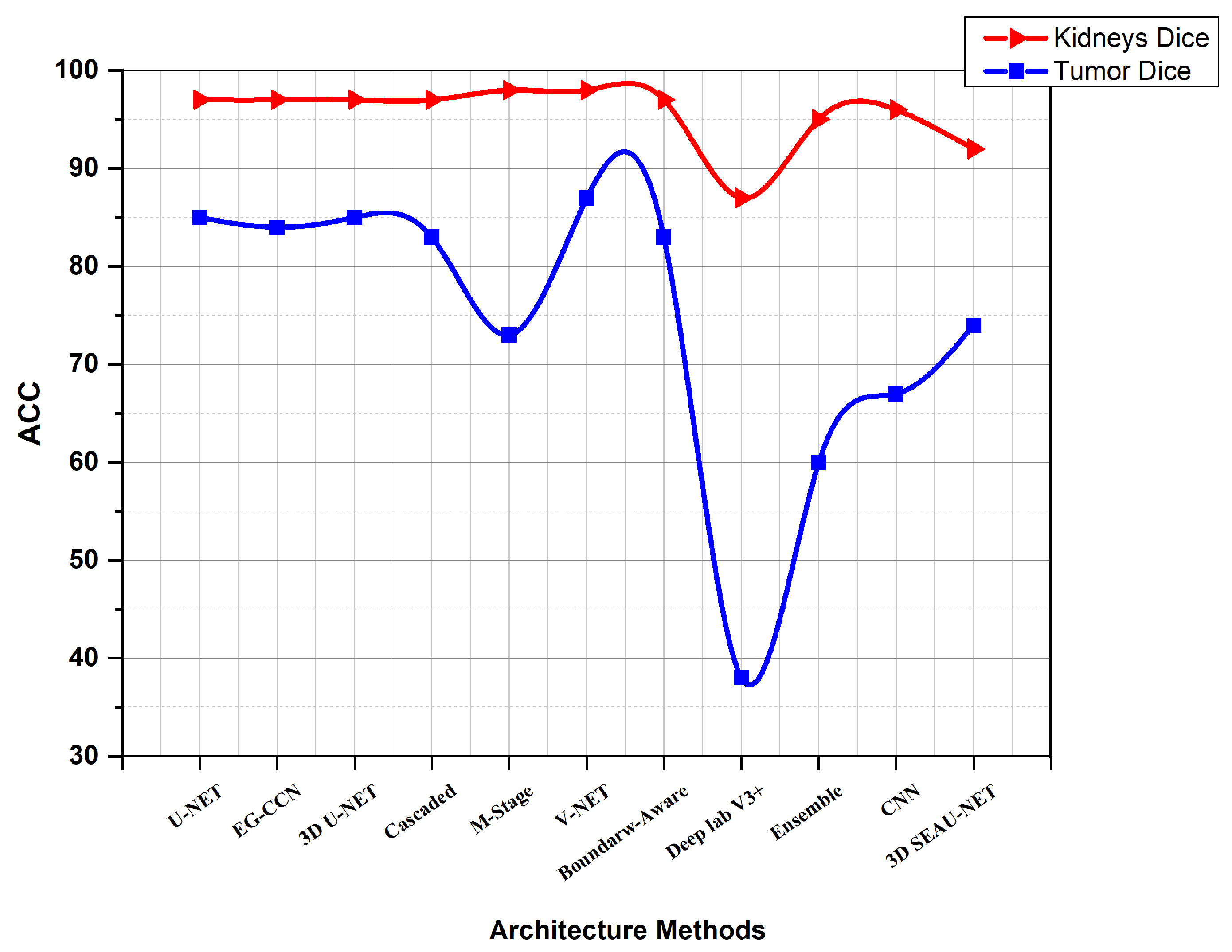
| [61] | 0.965 | 0.835 | 0.900 |
| [60] | 0.967 | 0.845 | 0.906 |
| [39] | 0.974 | 0.851 | 0.912 |
| [129] | 0.97 | 0.32 | |
| [59] | 0.974 | 0.831 | 0.902 |
| [12] | 0.969 | 0.805 | 0.887 |
| [62] | 0.98 | 0.73 | 0.855 |
| [40] | 0.977 | 0.865 | 0.921 |
| [19] | 0.973 | 0.817 | |
| [70] | 0.978 | 0.868 | 0.923 |
| [5] | 0.974 | 0.810 | 0.892 |
| [134] | 0.872 | 0.384 | |
| [41] | 0.968 | 0.743 | 0.856 |
| [47] | 0.949 | 0.601 | |
| [44] | 0.970 | 0.834 | 0.902 |
| [46] | 0.960 | 0.770 | |
| [66] | 0.930 | 0.570 | |
| [64] | 0.968 | 0.750 | |
| [45] | 0.964 | 0.674 | |
| [71] | 0.924 | 0.743 | |
| [72] | 0.852 | ||
| KiTS21 | |||
| [63] | 0.943 | 0.778 | |
| [49] | 0.975 | 0.881 | 0.871 |
| [53] | 0.923 | 0.553 | |
| [65] | 0.934 | 0.643 | |
| [67] | 0.96 | 0.81 | |
| [68] | 0.654 | ||
| [69] | 0.916 | 0.541 | |
| [55] | 0.937 | 0.750 | 825 |
| [56] | 0.90 | 0.39 | |
| Other Dataset | |||
| [50] | 0.859 | ||
| [54] | 0.923 | 0.826 | 0.875 |
| [51] | 0.925 | ||
Publisher’s Note: MDPI stays neutral with regard to jurisdictional claims in published maps and institutional affiliations. |
© 2022 by the authors. Licensee MDPI, Basel, Switzerland. This article is an open access article distributed under the terms and conditions of the Creative Commons Attribution (CC BY) license (https://creativecommons.org/licenses/by/4.0/).
Share and Cite
Abdelrahman, A.; Viriri, S. Kidney Tumor Semantic Segmentation Using Deep Learning: A Survey of State-of-the-Art. J. Imaging 2022, 8, 55. https://doi.org/10.3390/jimaging8030055
Abdelrahman A, Viriri S. Kidney Tumor Semantic Segmentation Using Deep Learning: A Survey of State-of-the-Art. Journal of Imaging. 2022; 8(3):55. https://doi.org/10.3390/jimaging8030055
Chicago/Turabian StyleAbdelrahman, Abubaker, and Serestina Viriri. 2022. "Kidney Tumor Semantic Segmentation Using Deep Learning: A Survey of State-of-the-Art" Journal of Imaging 8, no. 3: 55. https://doi.org/10.3390/jimaging8030055
APA StyleAbdelrahman, A., & Viriri, S. (2022). Kidney Tumor Semantic Segmentation Using Deep Learning: A Survey of State-of-the-Art. Journal of Imaging, 8(3), 55. https://doi.org/10.3390/jimaging8030055