Abstract
With the exponential growth of high-quality fake images in social networks and media, it is necessary to develop recognition algorithms for this type of content. One of the most common types of image and video editing consists of duplicating areas of the image, known as the copy-move technique. Traditional image processing approaches manually look for patterns related to the duplicated content, limiting their use in mass data classification. In contrast, approaches based on deep learning have shown better performance and promising results, but they present generalization problems with a high dependence on training data and the need for appropriate selection of hyperparameters. To overcome this, we propose two approaches that use deep learning, a model by a custom architecture and a model by transfer learning. In each case, the impact of the depth of the network is analyzed in terms of precision (P), recall (R) and F1 score. Additionally, the problem of generalization is addressed with images from eight different open access datasets. Finally, the models are compared in terms of evaluation metrics, and training and inference times. The model by transfer learning of VGG-16 achieves metrics about 10% higher than the model by a custom architecture, however, it requires approximately twice as much inference time as the latter.
1. Introduction
In recent years, the expansion of Internet services and the proliferation and strengthening of social platforms such as Facebook, Instagram and Reddit have had a significant impact on the amount of content circulating in digital media. According to the International Telecommunication Union (ITU), at the end of 2019, 53.6% of the world’s population uses the Internet, which means that approximately 4.1 billion people have access not only to this technology, but also to different tools available online [1]. Although in most cases the content shared is original or has only been manipulated for entertainment purposes, in other cases the manipulation may be intentional for disinformation purposes, with political and forensic repercussions, for example, using the fake content as digital evidence in a criminal investigation.
Image or video manipulation refers to any action that can be performed on a digital content using software editing tools (e.g., Adobe Photoshop, GIMP, PIXLR) or artificial intelligence. In particular, the copy-move technique copies a part of an image and then pastes it into the same image [2]. As editing tools advance, the quality of the fake images increases and they appear to the human eye as original images. In addition, post-processing manipulations, such as JPEG compression, brightness changes, or equalization, can reduce the traces left by manipulation and make it more difficult to detect [3].
The copy-move forgery detection (CMFD) includes hand-crafted and deep learning-based methods [2]. The former is mainly divided into block-based, keypoint-based and hybrid approach. The second uses custom architectures from scratch or fine-tuned models of pre-trained architectures such as VGG-16 [4]. Block-based approaches use different types of features extraction, for example, Fourier transform, DCT (Discrete Cosine Transform) [5,6] or Tetrolet transform [7]. One of their concerns is the reduction of performance when the copied object is rotated or resized, as the detection of counterfeiting is done through a matching process [8]. On the other hand, keypoint-based approaches such as SIFT (Scale Invariant Feature Transform) [9] and SURF (Speed-UP Robust Features) [10] are more robust to rotation and lighting variations but they have several challenges to overcome such as detecting counterfeits in regions of uniform intensity, natural duplicate objects detected as fake duplicate objects, and dependence on actual key points in the image [6]. A hybrid approach provided more stable results in terms of precision (P), recall (R) and F1 score, but only for a single data set [11].
Recent approaches use Convolutional Neural Network (CNN) for feature extraction and classification [12,13]. For example, a custom CNN with nine convolutional layers and a fully connected (FC) layer was proposed in [14]. The architecture was trained separately with CASIA v1 and CASIA v2 datasets, obtaining an accuracy of 98.04% and 97.83%, respectively. A similar work used a custom model with six convolutional layers and three FC layers, with batch normalization in all the convolutional layers, and dropout in the FC layers (except the last one); using the CoMoFoD dataset, the internal validation of this model reached an accuracy of 95.97% [15]. A less deep custom architecture uses only two convolutional layers and two FC layers [16]. The authors trained and validated the model with one, two and three datasets obtaining F1 scores of 90%, 94% and 95%, respectively. Although they address the problem of generalization, their mixed datasets are unbalanced, one with a ratio of 2:1 for fake and original images, and the other with a ratio of 2:3. Finally, a data-driven local descriptor with CNN obtained F1 scores between 0.5 and 0.7 for the CoMoFoD dataset [17].
Complementary to custom designs with CNNs, a second group of CNN-based approaches use transfer learning (TL). In this case, pre-trained models are used even for feature extraction or by means of fine-tuning. For example, a pre-trained AlexNet model is followed by a feature comparison block and a post-processing stage which provides F1 score of 93% for the GRIP dataset [18]. In other case, VGG-16 has been used as a feature extractor up to the last pooling layer [19]. Experiments were conducted with the MICC-F220 dataset reporting precision of 98%, recall of 89.5%, F1 score of 92% and accuracy of 95%.
Although there are many proposals that have addressed the problem of CMFD, concerns and challenges remain as listed below:
- Most classification models using deep learning have been trained and validated with a unique dataset, limiting their use to other kind of tampered images. In other words, they have not addressed the problem of generalization;
- The CNN models trained with various datasets did not use class-balanced data, so they could be biased to a particular class;
- Most methods did not report image prediction times, so it is not possible to know if they are suitable in applications that require real time or massive data analysis;
- The deep learning-based works have used a single design strategy, either custom or by transfer learning, but, to our knowledge, no work has compared the two approaches for the same dataset.
According to the above, this research makes a contribution in the following aspects:
- Two models of CMFD based on deep learning are proposed, one corresponding to custom design and the other by transfer learning. Additionally, the dependence of the depth of the network on the performance of the classifier is evaluated.
- The generalization problem is addressed by training and validating the proposed models with data from eight public datasets. Also, external validation results are also compared when the architecture is trained on a single dataset.
- Finally, the inference time of the custom model is compared with that of the VGG-16 based model.
The rest of the paper is organized as follows—Section 2 presents the proposed architectures by custom design and transfer learning. Section 3 describes the experimental tests and the models selected for each design strategy. Section 4 presents the results for the generalization problem, as well as the comparison between the proposed models in terms of performance metrics and inference times. Section 5 discusses the results. Finally, Section 6 summarises the work.
2. Proposed Architectures for CMFD
We propose two approaches for CMFD. The first uses a custom design and the second uses transfer learning. Both design strategies are based on CNNs. In the following, we will explain each case.
2.1. Architectures by Custom Design
In this design strategy, we considered that the features that allow us to identify whether an image is original or has been manipulated with the copy-move technique are not found in very deep layers, since high-level features such as shape are not useful to solve this kind of problem. This is supported by previous studies, which state that in terms of network depth, the number of convolutional layers plus the number of FC layers, should not exceed 10 layers [14,15,16]. In our design, we propose five architectures with different depths, up to five convolutional layers (conv) with two FC layers. Figure 1 shows the proposed architectures, where each block specifies the type of layer (i.e., conv, pooling (pool) or FC), the number of filters and the size of the kernel. For example, block1_conv, 32, is the first convolutional layer with 32 filters and kernel size of .
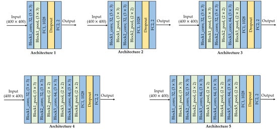
Figure 1.
Architectures by custom design: conv is the convolutional layer, pool is pooling layer, FC is the fully-connected layer.
In all cases, the input image is resized to . The first convolutional layer has 32 filters of size, with the Leaky_ReLU activation function using alpha = 0.09. In this layer, the padding is fixed as same, and the stride is 1 pixel. Its output is a feature map of , which has the same height (H) and width (W) of the input image, and the number of channels is equal to the number of filters. Next, the MaxPooling layer reduces the size of the input, that is, the feature map, in terms of H and W, but preserving the number of channels, according to Equation (1):
where is the ceiling function, k is the kernel size, s is the stride, p is the padding, is the height of the output, and is the weight of the output. With H = 400, W = 400, p = 0, k = 3 and s = 3, the output is .
Hence, the difference between the architectures is the number of convolutional layers. The second architecture has two conv+pool layers; the third architecture has three conv+pool layers; and so on. All convolutional layers have padding equal to same so the H and W values of the input feature maps are preserved. Except for the first MaxPooling layer, these blocks work with . The last two layers are fully-connected with 1028 and 2 units, respectively. Leaky_ReLU is used up to the penultimate layer, while softmax is used in the last layer.
Table 1 summarizes the hyperparameters of the five architectures by custom design. This table consists of four parts: the first part corresponds to the convolutional layers (from block1_conv to block5_pool); the second part corresponds to the FC1 layer; the third part corresponds to the FC2 layer; and the last part consolidates the five architectures.

Table 1.
Hyperparameters of the proposed architectures by custom design: k is the kernel size, s is stride, p is padding.
Regarding activation function, Leaky_ReLU is chosen to avoid the dying ReLU problem. The alpha value is fixed to 0.09 for convolutional layers, and 0.1 for the first FC layer. This activation function is calculated according to Equation (2).
where is the output of the activation function, and x is the input. Unlike the ReLU function, negative values are allowed at the output.
The second group of hyperparameters are related to the training stage. We have selected the following attributes: 80 epochs, categorical cross-entropy as loss function, SGD as the optimizer with a learning rate of 0.001 and a decay of 0.0001. Finally, with the purpose of reducing overfitting, we apply two strategies, dropout of 0.3 in the next-to-last layer, and image augmentation with horizontal and vertical flip.
2.2. Architectures by Transfer Learning (TL)
VGG-16 is one of the widely known models for image classification, which was trained with the sub-set of 1000 classes for the ImageNet Challenge [20]. The VGG architecture was proposed by the Visual Geometry Group of the University of Oxford and it is characterized by a stack of convolutional layers that precede a MaxPooling layer [21]. It has and filters, with a stride fixed to 1 pixel, and it includes 13 convolutional layers and 3 FC layers. Compared to the proposed architectures by custom design, VGG-16 differs in the depth of the network, in the number of filters in the convolutional layers, in the activation function, and also in the number of convolutional layers stacked before the pooling layer.
We have selected the pre-trained model VGG-16 for the following reasons:
- It is a sequential architecture as the proposed one, then we can compare the performance of the custom model with the model by transfer learning for the same type of architecture and analyze whether the features learned from a pre-trained model are useful for this type of classification problem;
- In recent work, some models by transfer learning with VGG-16 have been shown to be useful for identifying fake images from different types of manipulations such as copy-move [19] and colorization [12];
- Although VGG-16 is an architecture with a larger number of parameters and higher inference times than other architectures such as Inception or ResNet, it can be pruned for real-time applications without performance degradation [22].
Regarding transfer learning, there are several choices of using pre-trained models, one of them replaces part of the layers of the original architecture and preserves the others [13]. For instance, VGG-16 architecture can be preserved up to block4_pool layer and then add fully-connected layers with a different number of outputs. The new architecture will have pre-trained (frozen) parameters corresponding to those of the layers block1_conv1 to block4_pool, and trainable parameters corresponding to the new FC layers.
In our case, we tested the performance of four different architectures from VGG-16, that is, different frozen points. Figure 2 shows the architectures with this design strategy and Table 2 shows their corresponding hyperparameters. The first part corresponds to the architecture that was transferred from VGG-16 with its pre-trained parameters. The second part corresponds to the FC1 layer which depends on the frozen point. The third part is the FC2 layer. The last part is the total number of parameters for each of the four architectures, which includes the pre-trained parameters and the trainable parameters (i.e., FC1 + FC2). In all cases, the input image size is .
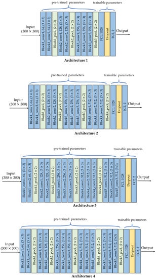
Figure 2.
Architectures by TL: conv is convolutional layer, pool is pooling layer, FC is fully-connected layer.

Table 2.
Hyperparameters of the architectures by transfer learning: k is the kernel size, s is stride, p is padding.
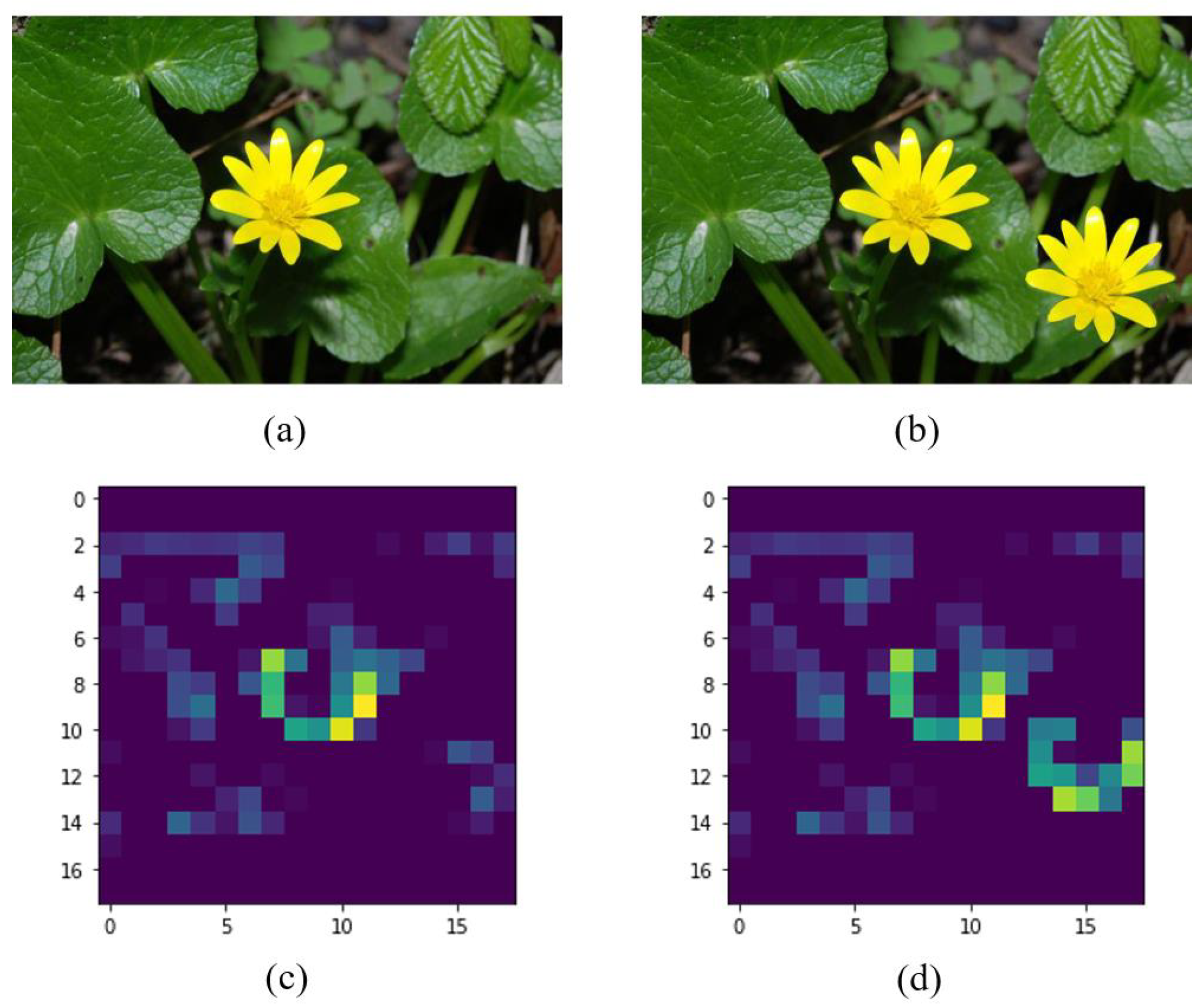
On the other hand, to illustrate the features learned by the VGG-16 pre-trained model, we have selected the block4_pool layer to display one of its feature maps. Figure 3 shows the example for the filter 60. Similar patterns are detected in the feature maps for the two flowers, that is, a green and yellow semi-circle appears in the corresponding areas that have flowers. This type of pattern allows the classifier to make the decision on the originality of the image.

Figure 3.
Example of feature maps for the block4_pool of the pre-trained VGG-16 model: (a) original image, (b) fake image with copy-move, (c) output of the filter 60 for the original image, (d) output of the filter 60 for the fake image. The source of (a,b) is [23] with permission of the authors.
Finally, to train the transfer-learning based model, the same hyperparameters defined for the custom architecture are selected: 80 epochs, categorical cross-entropy as loss function, SGD as the optimizer with a learning rate of 0.001 and a decay of 0.0001. However, in this case, the dropout value is 0.45.
3. Experimental Tests
Bearing in mind that one of the purposes of this research was to address the problem of generalization, it is mandatory to consider several datasets for model training. Then, a unified dataset should have diversity in image size, format, color space and editing quality, that is, whether the manipulation is perceptible or not. This is done by unifying several datasets, some of which have been widely used in the literature, while others are new. Specifically, we have selected eight datasets, as follows: Coverage, CG-1050 v1, CG-1050 v2, MICC-F220, MICC-F2000, Copy-move Forgery Dataset (CMFD), CASIA v1 and CASIA v2. Table 3 shows the characteristics of each dataset.

Table 3.
Characteristics of the selected datasets.
The unified dataset contains images in JPEG, BMP and TIF formats, color and grayscale images, different sizes of the copied object and different orientation. They were split in training, validation, and testing (60%, 20% and 20%, respectively). Additionally, all images were converted to JPEG format, to train the model using images with a lossy compression format. Table 4 shows the number of fake and original images taken from each dataset.

Table 4.
Unified dataset: number of images taken from single datasets.
It was necessary to add original images since some datasets only contained fake images. Table 5 shows the final distribution of the unified dataset, including 1308 original images obtained from a personal repository.

Table 5.
Distribution of the unified dataset: training, validation, and test.
As shown in Table 5, the unified dataset is balanced by class, so that the models are not biased towards a particular class.
3.1. Comparison Metrics
To compare the performance of the classifier, we use three metrics that are suitable for balanced datasets, such as the unified dataset, corresponding to precision (P), recall (R) and F1 score. Precision measures the ratio of images predicted as fake that belong to that class. Recall gives the ratio of fake images that are correctly classified. Finally, the F1 score is the harmonic mean between precision and recall. These metrics are obtained using Equations (3)–(5):
where TP is the number of True Positives, FP is the number of False Positives and FN is the number of False Negatives. The class fake is the positive class while the class original is the negative class.
In addition, we use accuracy (acc) to compare our results with some of the state-of-the-art proposals. This metric is obtained with Equation (6):
The four metrics range between 0 and 1, their ideal value is 1 and the worst is 0.
3.2. Impact of the Depth for the Custom Architecture
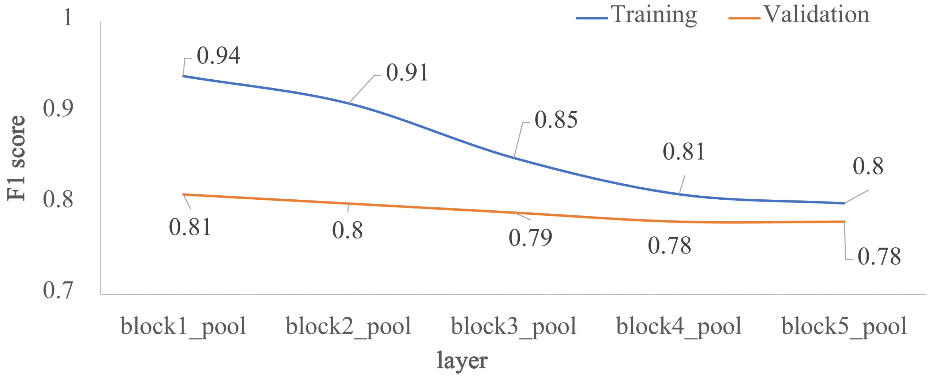
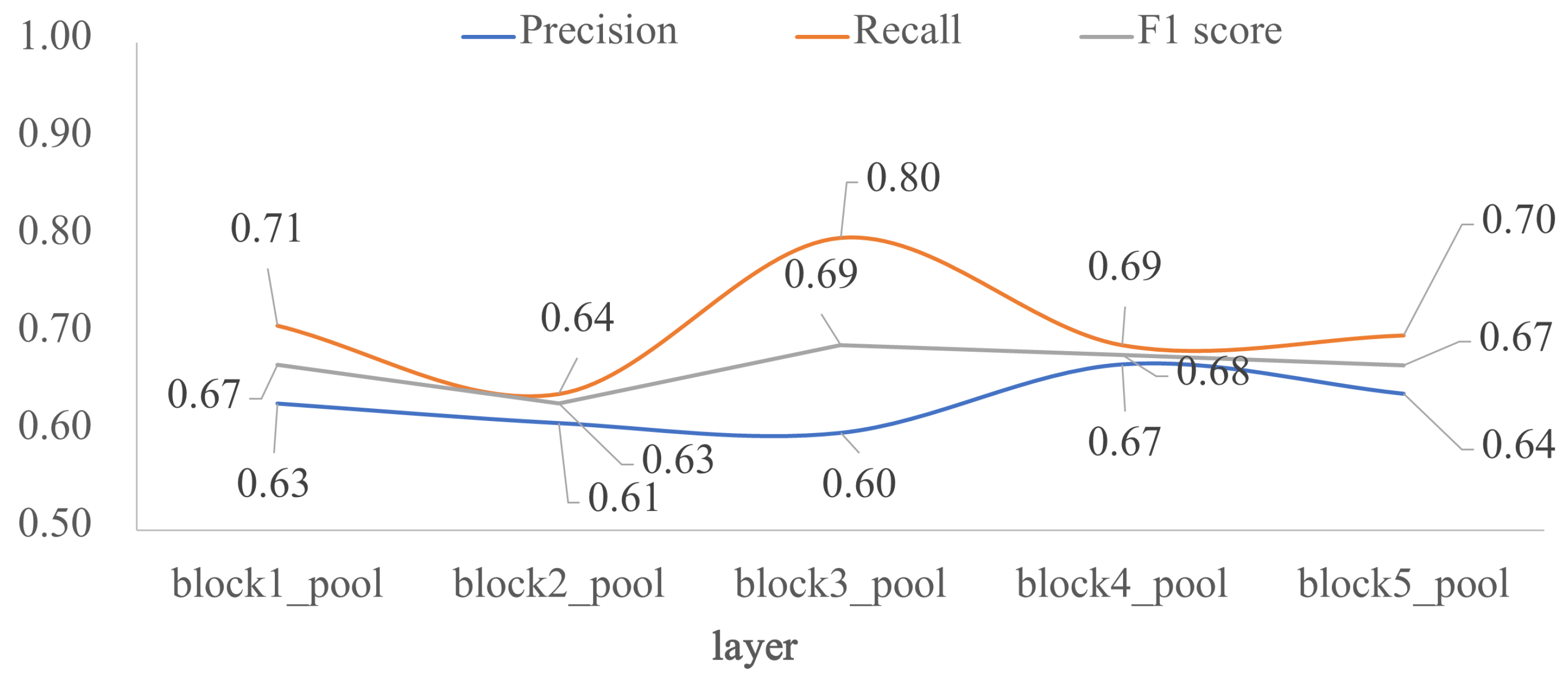
To assess how architecture depth affects model performance, we trained the five custom-designed architectures of Figure 1. As shown in Figure 4, model performance decreased as depth increased, the F1 scores are very similar between layers block4_pool and block5_pool with a very low overfitting. The impact of the depth of the architecture was also analyzed in terms of external validation with the test dataset, that is, using images unknown to the trained model. Figure 5 shows the behavior of F1 score, precision and recall by varying the number of convolutional layers. According to the results, block2_pool and block4_pool have the lowest variation in their metrics (P, R, F1), which means a better balance between precision and recall, however, the highest scores correspond to block4_pool.
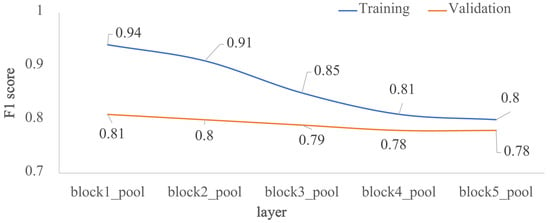
Figure 4.
Impact of the depth for the custom architecture in terms of F1 score: training vs validation. The x-axis corresponds to the last layer before the FC1 layer, and the y-axis is the F1 score.
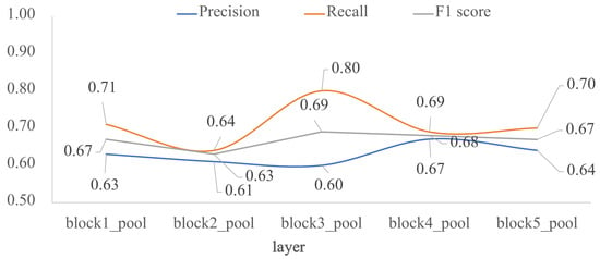
Figure 5.
Impact of the depth for the custom architecture in terms of P, R and F1 score: external test. The x-axis corresponds to the last layer before the FC1 layer, and the y-axis are the evaluated metrics.
Considering the above results, the proposed model by custom design was obtained from the architecture 4, that is, up to block4_pool with two FC layers.
3.3. Impact of the Depth for the Architecture by Transfer Learning
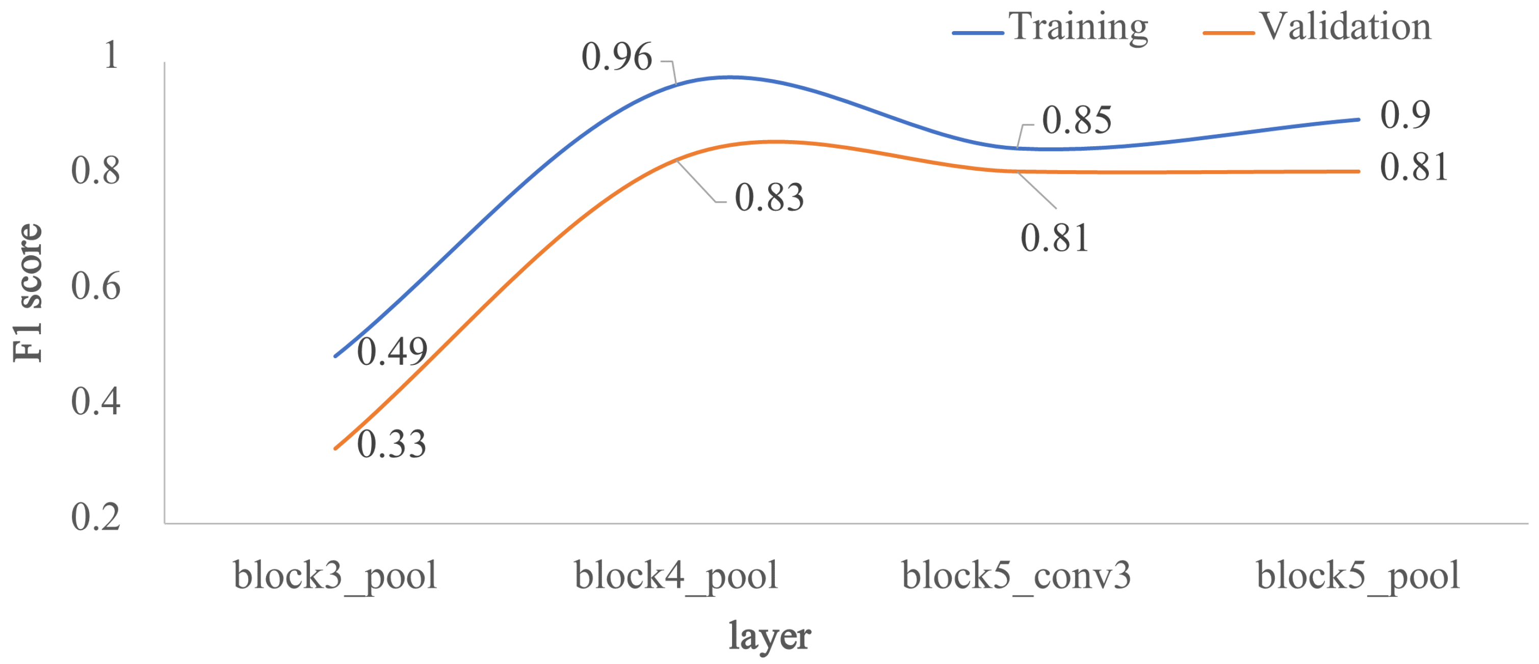
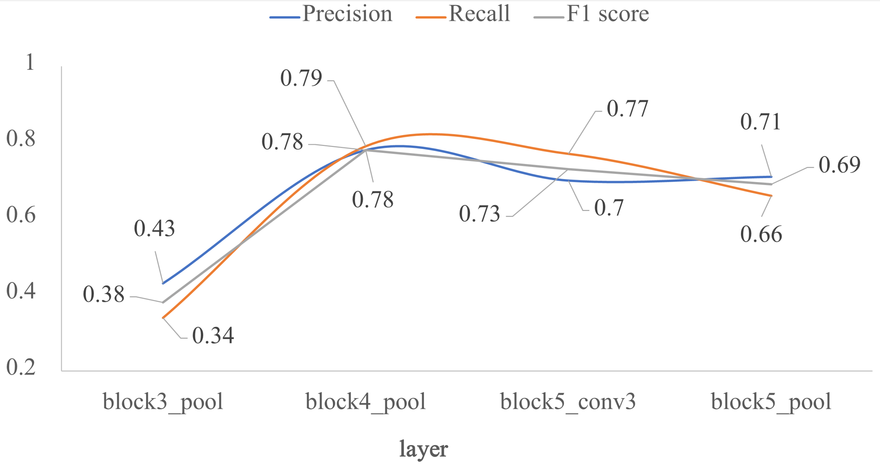
In the second approach, the four architectures in Figure 2 were evaluated, as it is shown in Figure 6. Each architecture corresponds to a specific freezing point of the pre-trained VGG-16 model: block3_pool, block4_pool, block5_conv3 and block5_pool. The worst metrics were obtained for the most superficial freezing layer, where the metrics for training and validation did not exceed 0.5. Using deeper freezing points, the F1 score in training exceeded 0.9 for block4_pool and block5_pool and 0.8 for block5_conv3. In validation, the F1 score presented values of 0.83, 0.81 and 0.81 for block4_pool, block5_conv3 and block5_pool, respectively. In summary, the F1 score did not increase when increasing the network freezing point beyond the block4_pool layer.
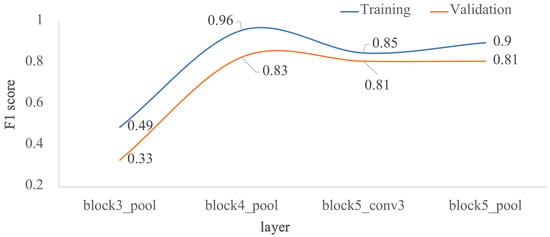
Figure 6.
Impact of the depth for the architecture by transfer learning using VGG-16, in terms of F1 score: training vs. validation. The x-axis corresponds to the selected last layer of VGG-16, and the y-axis is the F1 score.
Finally, the four models by transfer learning were validated with the test dataset. Figure 7 shows the results in terms of F1 score. For the block3_pool layer, the best metric is precision, but for the block5_conv3 layer the best metric is recall. The good balance between precision and recall is found in block4_pool layer in which P, R, and F1 score are very close among them. This layer is a breaking point in the performance of the classifier. As the freezing point gets deeper, the performance metrics decrease, being lower than 0.71 for the block5_pool layer.
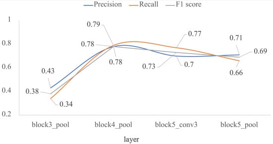
Figure 7.
Impact of the depth for the architecture by transfer learning using VGG-16, in terms of P, R and F1: external test. The x-axis corresponds to the selected last layer of VGG-16, and the y-axis are the evaluated metrics.
Therefore, the proposed model by transfer learning was obtained from the architecture 2, that is, up to block4_pool from VGG-16, plus two new FC layers.
4. Results
Considering that the TL-based model obtained better performance metrics than the custom-designed model (i.e., 0.78 vs 0.68 for F1 score), the TL-based model is selected for the generalization tests in Section 4.1 and Section 4.2. In addition, both models are compared in terms of performance, training and inference times, in Section 4.3.
4.1. Training with a Single Dataset
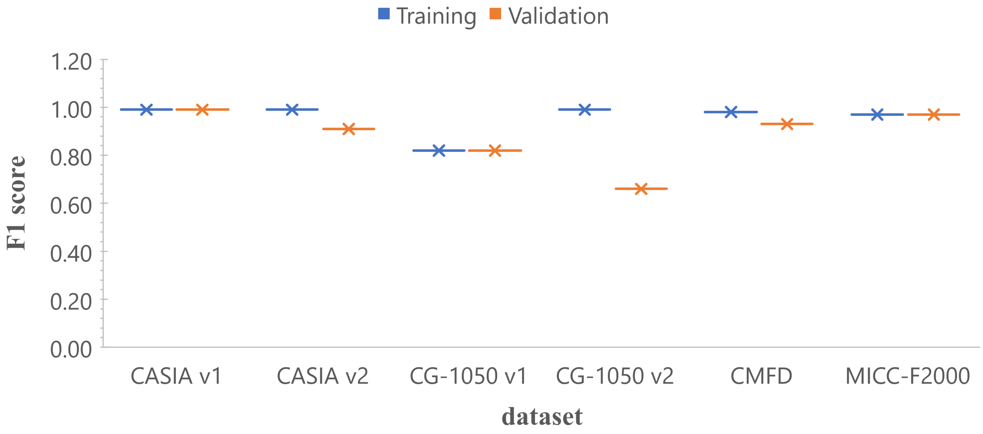
In this section we trained the architecture 2 of the TL-based strategy with six different datasets, (i.e., CASIA v1, CASIA v2, CG-1050 v1, CG-1050 v2, Copy-move forgery dataset (CMFD) and MICC-F2000), obtaining six different models. Figure 8 shows the results in terms of F1 score for training and validation. It should be noted that, for the datasets of CASIA v1, MICC-F2000 and CG-1050 v1, F1 scores are very close to each other for training and validation, and close to 1; while for CASIA v2 and CMFD, the values are higher than 0.9. Only, for the CG-1050 v2 dataset, the validation value is distant from the training one. In summary, the same architecture is able to obtain high scores for different datasets when the model is validated with data similar to those used in the training stage.
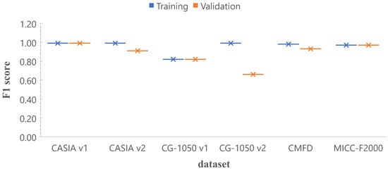
Figure 8.
Comparison in terms of F1 score with a single dataset (training vs. validation). The x-axis corresponds to the model trained with the specific dataset, and the y-axis is the F1 score.
The next step is to compare the results with those reported in the literature with a single dataset. Table 6 shows either the acc or the F1 score for some works, divided in three groups: CASIA (v1, v2), CMFD and MICC (F2000, F220, F600). For the copy-move forgery dataset (CMDF) group, the results were very similar between them. For the CASIA group, similar results are found for custom CNN and by transfer learning models. For the MICC group, deep learning-based methods outperform hand-crafted based methods. However, it is not clear whether the classifiers are biased to one class, as few papers report all four metrics: acc, P, R and F1. For instance, in [29] the authors reported a precision of 89.0% and recall of 100%, which implies that these metrics are not balanced, and specifically, the classifier is slightly biased to the positive class.

Table 6.
Comparison between state-of-the-art approaches in terms of accuracy (acc) and F1 score for the datasets: CASIA (v1, v2), CMFD and MICC (F2000, F220, F600). The higher the better.
Thus, our proposed TL-based model exceeds most of the results reported by other works, in two of the three groups of this comparison. It should be noted that transfer learning with VGG-16 had already been used for the same classification task (i.e., ref [19]) up to the block5_pool layer, but its results in terms of F1 score are lower than those of our work. This is because after the block4_pool layer the performance decreases, as is reported in Figure 7.
4.2. Adressing the Problem of Generalization
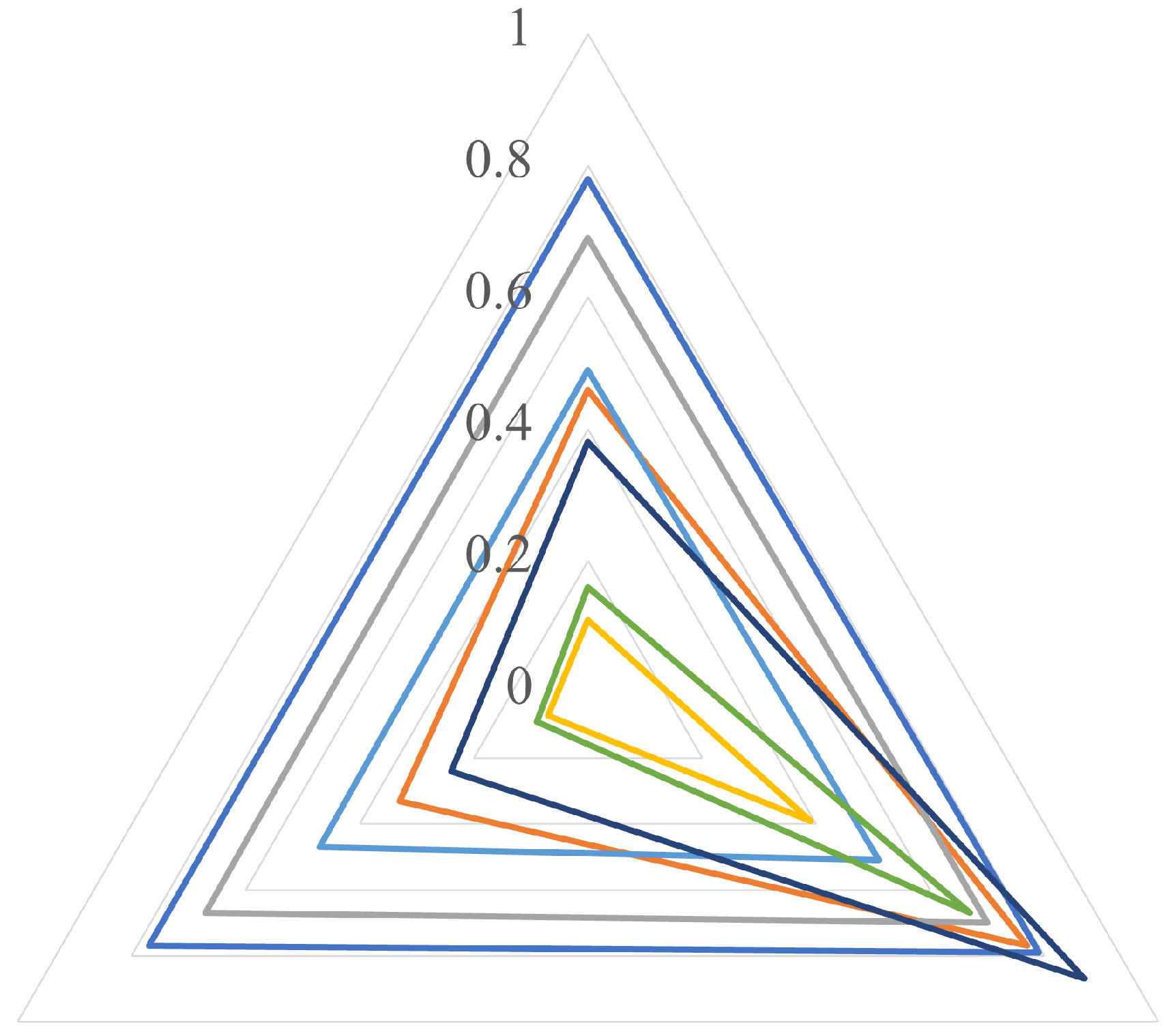
We evaluate the generalization capacity when the architecture by transfer learning is trained with a single dataset versus several datasets. We test the six models trained with a single dataset (Section 4.1) against the unified dataset, and we compare their results with the selected model of Section 3.3. Figure 9 shows a radar plot in which each vertex of the triangle corresponds to P (up), R (down, right) and F1 score (down, left). The best model is the one whose curve is the most external, without biasing any of the metrics.
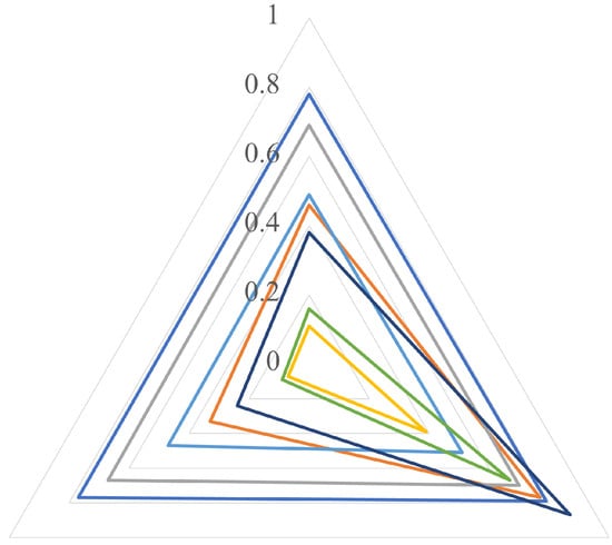
Figure 9.
Ability of generalization: single dataset vs. unified dataset (UD). The triangle represents P (up), R (down, right) and F1 score (down, left).
As shown in Figure 9, the outermost curve corresponds to the model trained with the unified dataset, in which there is an adequate balance between P and R, and therefore the three values (P, R and F1 score) are very similar between them. The second place is occupied by the model trained with CASIA v2 in which again the metrics are balanced but are lower than in the first case. One of the worst curves was found with the model trained with CMFD dataset, in which R is high but P is low. This means that few fake images are labelled as original, but many original images are labelled as fake.
According to the above, not only the results for individual datasets are important to know the quality of the model, but also the generalization results. An architecture trained and evaluated on a single dataset can achieve high F1 score values, but it is no guarantee of high performance for new images.
4.3. Custom Model vs. Vgg-16 Based Model
In this last test section, we compare the two proposed models in terms of performance (Table 7), number of parameters (Table 8) and training and inference times (Table 9).

Table 7.
Comparison of the two proposed models in terms of acc, P, R and F1 score.

Table 8.
Comparison of the two proposed models in terms of number of parameters.

Table 9.
Comparison of the two proposed models in terms of training and validation times, h is hours, sec is seconds.
In terms of performance, the model by transfer learning shows higher scores in all four statistics. However, in both models, there is a high trade-off between accuracy and recall, and therefore, the amount of misclassifications is similar for the two classes (original and fake).
In the second comparison, all parameters are trainable in the custom architectures, while only the FC layer parameters are trainable in the architectures by transfer learning. In the first case, architecture 4 from Table 1 was selected, while in the second case, architecture 2 from Table 2 was selected. As shown in Table 8, the total number of parameters of the second approach is much higher than the former.
On the other hand, in terms of training and inference times (Table 9), the model by custom architecture uses about 65% of that of the transfer-learning-based.
In summary, the model by the custom architecture has a lower number of parameters than the model by transfer learning, with less inference time, but with a lower success rate in the classification.
5. Discussion
This research addressed the generalization problem, where models trained with a single dataset can show very high results with similar data, but their performance decreases significantly with data dissimilar to that of the training stage. In most papers, copy forgery detection models have been trained and validated (internally) with a single dataset or with datasets from the same “family”, for example, CASIA (v1 and v2) or MICC (2000, F220 F600), but not with data from multiple and highly diverse datasets.
Fitting the model for single datasets is not a very difficult task, as presented in Figure 8, where the same architecture was used to train six single models with high results in five of the six cases. However, in a real scenario, the trained models must classify images dissimilar to those used in the training stage, and then, models trained with a single data set do not perform adequately, as was shown in Figure 9. For instance, the model trained with the CMFD dataset obtained F1 scores close to 1 when evaluated with images from the same dataset, but its performance decreased when tested with images from other datasets showing high recall and very low precision.
For this reason, to approach a real scenario, we used a unified dataset from different individual datasets, some of which have already been used in other works and others are new, with a high diversity as summarized in Table 3. Obtaining a trained model with high precision and recall, and a proper balance between these two metrics was not an easy task, so it was necessary to evaluate several hyperparameters. After several adjustments of the hyperparameters (both related to the architecture as well as the training stage) we obtained two promising models, which are presented in this paper.
It is worth noting that the task of copy-move forgery detection is not yet solved, because every day in social networks new high quality manipulated images are found, which could be classified not only by an algorithm but by human beings as originals.
6. Conclusions
In this paper we proposed two deep learning-based models, a custom model and a TL-based model, to evaluate its effectiveness in the CMFD task. Additionally, we address the generalization problem when the architecture is trained only with one dataset but tested with several datasets versus the approach trained with a large dataset. Finally, we evaluate not only the performance of the proposed models but their training and inference times. According to our results, the custom architecture with few convolutional layers have greater generalization problems than those with more layers; however, in the VGG-16 pre-trained model it was found that when using a freezing point beyond the block4_pool layer the classifier results get worse. Additionally, it was found that models trained with a single dataset tend to classify images into a single class (original or fake), such that P and R metrics are not balanced (one high and one low). The best balance between these metrics was obtained when the weights of the pre-trained VGG-16 model were frozen in the block4_pool layer and the unified dataset was used. Besides, the improved performance in classifying original and fake images in the VGG-16 based model has a direct relationship with the inference time, which is almost double that of the custom model.
Future work may consider extending the training dataset, assessing the impact of other hyperparameters on classifier performance and a hybrid approach mixing an image pre-processing stage using domain transformation (e.g., DFT, DCT, and DWT) with feature extraction based on deep learning.
Author Contributions
Conceptualization, D.M.B. and D.R.; methodology, Y.R.-O. and D.M.B. and D.R.; software, Y.R.-O. and D.M.B.; validation, Y.R.-O.; formal analysis, D.M.B.; investigation, D.M.B. and D.R.; data curation, Y.R.-O.; writing—original draft preparation, Y.R.-O. and D.M.B.; writing—review and editing, D.R.; visualization, D.M.B.; supervision, D.M.B. and D.R. All authors have read and agreed to the published version of the manuscript.
Funding
This research was funded by “Vicerrectoría de Investigaciones—Universidad Militar Nueva Granada”, grant number IMP-ING-2936 of 2019–2021.
Institutional Review Board Statement
Not applicable.
Informed Consent Statement
Not applicable.
Data Availability Statement
The data CG-1050 used in this study are openly available in [25,26].
Conflicts of Interest
The authors declare no conflict of interest.
Abbreviations
The following abbreviations are used in this manuscript:
| acc | Accuracy |
| CNN | Convolutional Neural Network |
| CMFD | Copy-Move Forgery Detection |
| conv | Convolutional layer |
| DCT | Discrete Cosine Transform |
| DFT | Discrete Fourier Transform |
| DWT | Discrete Wavelet Transform |
| FC | Fully-Connected |
| P | Precison |
| pool | Pooling layer |
| R | Recall |
| SIFT | Scale Invariant Feature Transform |
| SURF | Speed-Up Robust Features |
References
- ITU. Statistics. Available online: https://www.itu.int/en/ITU-D/Statistics/Pages/stat/default.aspx (accessed on 4 December 2020).
- Thakur, R.; Rohilla, R. Recent Advances in Digital Image Manipulation Detection Techniques: A brief Review. Forensic Sci. Int. 2020, 312, 110311. [Google Scholar] [CrossRef]
- Abd Warif, N.B.; Wahab, A.W.A.; Idris, M.Y.I.; Ramli, R.; Salleh, R.; Shamshirband, S.; Choo, K.K.R. Copy-move forgery detection: Survey, challenges and future directions. J. Netw. Comput. Appl. 2016, 75, 259–278. [Google Scholar] [CrossRef]
- Ferreira, W.D.; Ferreira, C.B.; da Cruz Júnior, G.; Soares, F. A review of digital image forensics. Comput. Electr. Eng. 2020, 85, 106685. [Google Scholar] [CrossRef]
- Dua, S.; Singh, J.; Parthasarathy, H. Detection and localization of forgery using statistics of DCT and Fourier components. Signal Process. Image Commun. 2020, 82, 115778. [Google Scholar] [CrossRef]
- Gani, G.; Qadir, F. A robust copy-move forgery detection technique based on discrete cosine transform and cellular automata. J. Inf. Secur. Appl. 2020, 54, 102510. [Google Scholar] [CrossRef]
- Meena, K.B.; Tyagi, V. A copy-move image forgery detection technique based on tetrolet transform. J. Inf. Secur. Appl. 2020, 52, 102481. [Google Scholar] [CrossRef]
- Sharma, S.; Ghanekar, U. A hybrid technique to discriminate Natural Images, Computer Generated Graphics Images, Spliced, Copy Move tampered images and Authentic images by using features and ELM classifier. Optik 2018, 172, 470–483. [Google Scholar] [CrossRef]
- Alberry, H.A.; Hegazy, A.A.; Salama, G.I. A fast SIFT based method for copy move forgery detection. Future Comput. Inform. J. 2018, 3, 159–165. [Google Scholar] [CrossRef]
- Badr, A.; Youssif, A.; Wafi, M. A Robust Copy-Move Forgery Detection In Digital Image Forensics Using SURF. In Proceedings of the 2020 8th International Symposium on Digital Forensics and Security (ISDFS), Beirut, Lebanon, 1–2 June 2020; pp. 1–6. [Google Scholar]
- Tinnathi, S.; Sudhavani, G. An Efficient Copy Move Forgery Detection Using Adaptive Watershed Segmentation withAGSO and Hybrid Feature Extraction. J. Vis. Commun. Image Represent. 2020, 74, 102966. [Google Scholar] [CrossRef]
- Ulloa, C.; Ballesteros, D.M.; Renza, D. Video Forensics: Identifying Colorized Images Using Deep Learning. Appl. Sci. 2021, 11, 476. [Google Scholar] [CrossRef]
- Pachón, C.; Ballesteros, D.M.; Renza, D. Fake Banknote Recognition Using Deep Learning. Appl. Sci. 2021, 11, 1281. [Google Scholar] [CrossRef]
- Rao, Y.; Ni, J. A deep learning approach to detection of splicing and copy-move forgeries in images. In Proceedings of the 2016 IEEE International Workshop on Information Forensics and Security (WIFS), Abu Dhabi, United Arab Emirates, 4–7 December 2016; pp. 1–6. [Google Scholar]
- Thakur, R.; Rohilla, R. Copy-Move Forgery Detection using Residuals and Convolutional Neural Network Framework: A Novel Approach. In Proceedings of the 2019 2nd International Conference on Power Energy, Environment and Intelligent Control (PEEIC), Greater Noida, India, 18–19 October 2019; pp. 561–564. [Google Scholar]
- Kumar, S.; Gupta, S.K. A Robust Copy Move Forgery Classification Using End to End Convolution Neural Network. In Proceedings of the 2020 8th International Conference on Reliability, Infocom Technologies and Optimization (Trends and Future Directions) (ICRITO), Noida, India, 4–5 June 2020; pp. 253–258. [Google Scholar]
- Liu, Y.; Guan, Q.; Zhao, X. Copy-move forgery detection based on convolutional kernel network. Multimed. Tools Appl. 2018, 77, 18269–18293. [Google Scholar] [CrossRef]
- Muzaffer, G.; Ulutas, G. A new deep learning-based method to detection of copy-move forgery in digital images. In Proceedings of the 2019 Scientific Meeting on Electrical-Electronics & Biomedical Engineering and Computer Science (EBBT), Istanbul, Turkey, 24–26 April 2019; pp. 1–4. [Google Scholar]
- Agarwal, R.; Verma, O.P. An efficient copy move forgery detection using deep learning feature extraction and matching algorithm. Multimed. Tools Appl. 2019, 79, 7355–7376. [Google Scholar] [CrossRef]
- Russakovsky, O.; Deng, J.; Su, H.; Krause, J.; Satheesh, S.; Ma, S.; Huang, Z.; Karpathy, A.; Khosla, A.; Bernstein, M.; et al. Imagenet large scale visual recognition challenge. Int. J. Comput. Vis. 2015, 115, 211–252. [Google Scholar] [CrossRef]
- Simonyan, K.; Zisserman, A. Very deep convolutional networks for large-scale image recognition. arXiv 2014, arXiv:1409.1556. [Google Scholar]
- He, Y.; Zhang, X.; Sun, J. Channel pruning for accelerating very deep neural networks. In Proceedings of the IEEE International Conference on Computer Vision, Venice, Italy, 22–29 October 2017; pp. 1389–1397. [Google Scholar]
- Ardizzone, E.; Bruno, A.; Mazzola, G. Copy–move forgery detection by matching triangles of keypoints. IEEE Trans. Inf. Forensics Secur. 2015, 10, 2084–2094. [Google Scholar] [CrossRef]
- Wen, B.; Zhu, Y.; Subramanian, R.; Ng, T.T.; Shen, X.; Winkler, S. COVERAGE—A novel database for copy-move forgery detection. In Proceedings of the 2016 IEEE International Conference on Image Processing (ICIP), Phoenix, AZ, USA, 25–28 September 2016; pp. 161–165. [Google Scholar]
- Castro, M.; Ballesteros, D.M.; Renza, D. A dataset of 1050-tampered color and grayscale images (CG-1050). Data Brief 2020, 28, 104864. [Google Scholar] [CrossRef]
- Castro, M.; Ballesteros, D.M.; Renza, D. CG-1050 v2: Original and Tampered Images. 2019. Available online: https://data.mendeley.com/datasets/28xhc4kyfp/1 (accessed on 17 December 2020).
- Amerini, I.; Ballan, L.; Caldelli, R.; Del Bimbo, A.; Serra, G. A sift-based forensic method for copy–move attack detection and transformation recovery. IEEE Trans. Inf. Forensics Secur. 2011, 6, 1099–1110. [Google Scholar] [CrossRef]
- Dong, J.; Wang, W.; Tan, T. Casia image tampering detection evaluation database. In Proceedings of the 2013 IEEE China Summit and International Conference on Signal and Information Processing, Beijing, China, 6–10 July 2013; pp. 422–426. [Google Scholar]
- Goel, N.; Kaur, S.; Bala, R. Dual branch convolutional neural network for copy move forgery detection. IET Image Process. 2021, 15, 656–665. [Google Scholar] [CrossRef]
- Chen, H.; Yang, X.; Lyu, Y. Copy-move forgery detection based on keypoint clustering and similar neighborhood search algorithm. IEEE Access 2020, 8, 36863–36875. [Google Scholar] [CrossRef]
- Elaskily, M.A.; Elnemr, H.A.; Sedik, A.; Dessouky, M.M.; El Banby, G.M.; Elshakankiry, O.A.; Khalaf, A.A.; Aslan, H.K.; Faragallah, O.S.; Abd El-Samie, F.E. A novel deep learning framework for copy-moveforgery detection in images. Multimed. Tools Appl. 2020, 79, 19167–19192. [Google Scholar] [CrossRef]
- Yu, L.; Han, Q.; Niu, X. Feature point-based copy-move forgery detection: Covering the non-textured areas. Multimed. Tools Appl. 2016, 75, 1159–1176. [Google Scholar] [CrossRef]
Publisher’s Note: MDPI stays neutral with regard to jurisdictional claims in published maps and institutional affiliations. |
© 2021 by the authors. Licensee MDPI, Basel, Switzerland. This article is an open access article distributed under the terms and conditions of the Creative Commons Attribution (CC BY) license (http://creativecommons.org/licenses/by/4.0/).


