Article

Quantitative Comparison of Deep Learning-Based Image Reconstruction Methods for Low-Dose and Sparse-Angle CT Applications

by
Johannes Leuschner
1,*,†,
Maximilian Schmidt
1,†,
Poulami Somanya Ganguly
2,3,
Vladyslav Andriiashen
2,
Sophia Bethany Coban
2,
Alexander Denker
1,
Dominik Bauer
4,
Amir Hadjifaradji
5,
Kees Joost Batenburg
2,6,
Peter Maass
1 and
Maureen van Eijnatten
2,7,*
1
Center for Industrial Mathematics, University of Bremen, Bibliothekstr. 5, 28359 Bremen, Germany
2
Centrum Wiskunde & Informatica, Science Park 123, 1098 XG Amsterdam, The Netherlands
3
The Mathematical Institute, Leiden University, Niels Bohrweg 1, 2333 CA Leiden, The Netherlands
4
Computer Assisted Clinical Medicine, Heidelberg University, Theodor-Kutzer-Ufer 1-3, 68167 Mannheim, Germany
5
School of Biomedical Engineering, University of British Columbia, 2222 Health Sciences Mall, Vancouver, BC V6T 1Z3, Canada
6
Leiden Institute of Advanced Computer Science, Niels Bohrweg 1, 2333 CA Leiden, The Netherlands
7
Department of Biomedical Engineering, Eindhoven University of Technology, Groene Loper 3, 5612 AE Eindhoven, The Netherlands
*
Authors to whom correspondence should be addressed.
These authors contributed equally to this work.
J. Imaging 2021, 7(3), 44; https://doi.org/10.3390/jimaging7030044
Submission received: 29 January 2021 / Revised: 21 February 2021 / Accepted: 22 February 2021 / Published: 2 March 2021
(This article belongs to the Special Issue Deep Learning in Medical Image Analysis)

Abstract

:
The reconstruction of computed tomography (CT) images is an active area of research. Following the rise of deep learning methods, many data-driven models have been proposed in recent years. In this work, we present the results of a data challenge that we organized, bringing together algorithm experts from different institutes to jointly work on quantitative evaluation of several data-driven methods on two large, public datasets during a ten day sprint. We focus on two applications of CT, namely, low-dose CT and sparse-angle CT. This enables us to fairly compare different methods using standardized settings. As a general result, we observe that the deep learning-based methods are able to improve the reconstruction quality metrics in both CT applications while the top performing methods show only minor differences in terms of peak signal-to-noise ratio (PSNR) and structural similarity (SSIM). We further discuss a number of other important criteria that should be taken into account when selecting a method, such as the availability of training data, the knowledge of the physical measurement model and the reconstruction speed.

1. Introduction

Computed tomography (CT) is a widely used (bio)medical imaging modality, with various applications in clinical settings, such as diagnostics [1], screening [2] and virtual treatment planning [3,4], as well as in industrial [5] and scientific [6,7,8] settings. One of the fundamental aspects of this modality is the reconstruction of images from multiple X-ray measurements taken from different angles. Because each X-ray measurement exposes the sample or patient to harmful ionizing radiation, minimizing this exposure remains an active area of research [9]. The challenge is to either minimize the dose per measurement or the total number of measurements while maintaining sufficient image quality to perform subsequent diagnostic or analytic tasks.
To date, the most common classical methods used for CT image reconstruction are filtered back-projection (FBP) and iterative reconstruction (IR) techniques. FBP is a stabilized and discretized version of the inverse Radon transform, in which 1D projections are filtered by the 1D Radon kernel (back-projected) in order to obtain a 2D signal [10,11]. FBP is very fast, but is not suitable for limited-data or sparse-angle setups, resulting in various imaging artifacts, such as streaking, stretching, blurring, partial volume effects, or noise [12]. Iterative reconstruction methods, on the other hand, are computationally intensive but are able to incorporate a priori information about the system during reconstruction. Many iterative techniques are based on statistical methods such as Markov random fields or regularization methods where the regularizers are designed and incorporated into the problem of reconstruction mathematically [13]. A popular choice for the regularizer is total variation (TV) [14,15]. Another well-known iterative method suitable for large-scale tomography problems is the conjugate gradient method applied to solve the least squares problem (CGLS) [16].
When classical techniques such as FBP or IR are used to reconstruct low-dose CT images, the image quality often deteriorates significantly in the presence of increased noise. Therefore, the focus is shifting towards developing reconstruction methods in which a single or multiple component(s), or even the entire reconstruction process is performed using deep learning [17]. Generally data-driven approaches promise fast and/or accurate image reconstruction by taking advantage of a large number of examples, that is, training data.
The methods that learn parts of the reconstruction process can be roughly divided into learned regularizers, unrolled iterative schemes, and post-processing of reconstructed CT images. Methods based on learned regularizers work on the basis of learning convolutional filters from the training data that can subsequently be used to regularize the reconstruction problem by plugging into a classical iterative optimization scheme [18]. Unrolled iterative schemes go a step further in the sense that they “unroll” the steps of the iterative scheme into a sequence of operations where the operators are replaced with convolutional neural networks (CNNs). A recent example is the learned primal-dual algorithm proposed by Adler et al. [19]. Finally, various post-processing methods have been proposed that correct noisy images or those with severe artifacts in the image domain [20]. Examples are improving tomographic reconstruction from limited data using a mixed-scale dense (MS-D) CNN [21], U-Net [22] or residual encoder-decoder CNN (RED-CNN) [23], as well as CT image denoising techniques [24,25]. Somewhat similar are the methods that can be trained in a supervised manner to improve the measurement data in the sinogram domain [26].
The first fully end-to-end learned reconstruction method was the automated transform by the manifold approximation (AUTOMAP) algorithm [27] developed for magnetic resonance (MR) image reconstruction. This method directly learns the (global) relation between the measurement data and the image, that is, it replaces the Radon or Fourier transform with a neural network. The disadvantages of this approach are the large memory requirements, as well as the fact that it might not be necessary to learn the entire transformation from scratch because an efficient analytical transform is already available. A similar approach for CT reconstruction was iRadonMAP proposed by He et al. [28], who developed an interpretable framework for Radon inversion in medical X-ray CT. In addition, Li et al. [29] proposed an end-to-end reconstruction framework for Radon inversion called iCT-Net, and demonstrated its advantages in solving sparse-view CT reconstruction problems.
The aforementioned deep learning-based CT image reconstruction methods differ greatly in terms of which component of the reconstruction task is learned and in which domain the method operates (image or sinogram domain), as well as the computational and data-related requirements. As a result, it remains difficult to compare the performance of deep learning-based reconstruction methods across different imaging domains and applications. Thorough comparisons between different reconstruction methods are further complicated by the lack of sufficiently large benchmarking datasets, including ground truth reconstructions, for training, validation, and testing. CT manufacturers are typically very reluctant in making raw measurement data available for research purposes, and privacy regulations for making medical imaging data publicly available are becoming increasingly strict [30,31].

1.1. Goal of This Study

The aim of this study is to quantitatively compare the performance of classical and deep learning-based CT image reconstruction methods on two large, two-dimensional (2D) parallel-beam CT datasets that were specifically created for this purpose. We opted for a 2D parallel-beam CT setup to facilitate large-scale experiments with many example images, whereas the underlying operators in the algorithms have straightforward generalizations to other geometries. We focus on two reconstruction tasks with high relevance and impact—the first task is the reconstruction of low-dose medical CT images, and the second is the reconstruction of sparse-angle CT images.

1.1.1. Reconstruction of Low-Dose Medical CT Images

In order to compare (learned) reconstruction techniques in a low-dose CT setup, we use the low-dose parallel beam (LoDoPaB) CT dataset [32]. This dataset contains 42,895 two-dimensional CT images and corresponding simulated low-intensity measurements. The ground truth images of this dataset are human chest CT reconstructions taken from the LIDC/IDRI database [33]. These scans had been acquired with a wide range of scanners and models. The initial image reconstruction for creating the LIDC/IDRI database was performed with different convolution kernels, depending on the manufacturer. Poisson noise is applied to the simulated projection data to model the low intensity setup. A more detailed description can be found in Section 2.1.

1.1.2. Reconstruction of Sparse-Angle CT Images

When using X-ray tomography in high-throughput settings (i.e., scanning multiple objects per second) such as quality control, luggage scanning or inspection of products on conveyor belts, very few X-ray projections can be acquired for each object. In such settings, it is essential to incorporate a priori information about the object being scanned during image reconstruction. In order to compare (learned) reconstruction techniques for this application, we reconstruct parallel-beam CT images of apples with internal defects using as few measurements as possible. We experimented with three different noise settings: noise-free, Gaussian noise, and scattering noise. The generation of the datasets is described in Section 2.2.

2. Dataset Description

For both datasets, the simulation model uses a 2D parallel beam geometry for the creation of the measurements. The attenuation of the X-rays is simulated using the Radon transform [10]
A x ( s , φ ) : = R x s cos ( φ ) sin ( φ ) + t sin ( φ ) cos ( φ ) d t ,
where s R is the distance from the origin and φ [ 0 , π ) the angle of the beam (cf. Figure 1). Mathematically, the image is transformed into a function of ( s , φ ) . For each fixed angle φ the 2D image x is projected onto a line parameterized by s, namely the X-ray detector.
A detailed description of both datasets is given below. Their basic properties are also summarized in Table 1.

2.1. LoDoPaB-CT Dataset

The LoDoPaB-CT dataset [32] is a comprehensive collection of reference reconstructions and simulated low-dose measurements. It builds upon normal-dose thoracic CT scans from the LIDC/IDRI Database [33,35], whereby quality-assessed and processed 2D reconstructions are used as a ground truth. LoDoPaB features more than 40,000 scan slices from around 800 different patients. The dataset can be used for the training and evaluation of all kinds of reconstruction methods. LoDoPaB-CT has a predefined division into four parts, where each subset contains images from a distinct and randomly chosen set of patients. Three parts were used for training, validation and testing, respectively. It also contains a special challenge set with scans from 60 different patients. The ground truth images are undisclosed, and the patients are only included in this set. The challenge set is used for the evaluation of the model performance in this paper. Overall, the dataset contains 35,820 training images, 3522 validation images, 3553 test images and 3678 challenge images.
Low-intensity measurements suffer from an increased noise level. The main reason is so called quantum noise. It stems from the process of photon generation, attenuation and detection. The influence on the number of detected photons N ˜ 1 can be modeled, based on the mean photon count without attenuation N 0 and the Radon transform (1), by a Poisson distribution [36]
N ˜ 1 ( s , φ ) Pois ( N 0 exp ( A x ( s , φ ) ) ) .
The model has to be discretized concerning s and φ for the simulation process. In this case, the Radon transform (1) becomes a finite-dimensional linear map A : R n R m , where n is the number of image pixels and m is the product of the number of detector pixels and the number of discrete angles. Together with the Poisson noise, the discrete simulation model is given by
A x + 𝕖 ( A x ) = 𝕪 δ , 𝕖 ( A x ) = A x ln ( N ˜ 1 / N 0 ) , N ˜ 1 Pois ( N 0 exp ( A x ) ) .
A single realization y δ R m of 𝕪 δ is observed for each ground truth image, x = x R n . After the simulation according to (3), all data pairs ( y δ , x ) have been divided by μ max = 81.35858 to normalize the image values to the range [ 0 , 1 ] . In the following sections, 𝕪 θ , y δ and x denote the normalized values.
The LoDoPaB ground truth images have a resolution of 362   p x × 362   p x on a domain of size 26   c m × 26   c m . The scanning setup consists of 513 equidistant detector pixels s spanning the image diameter and 1000 equidistant angles φ between 0 and π . The mean photon count per detector pixel without attenuation is N 0 = 4096 . The sampling ratio between the size of the measurements and the images is around 3.9 (oversampling case).

2.2. Apple CT Datasets

The Apple CT datasets [37] are a collection of ground truth reconstructions and simulated parallel beam data with various noise types and angular range sampling. The data is intended for benchmarking different algorithms and is particularly suited for use in deep learning settings due to the large number of slices available.
A total of 94 apples were scanned at the Flex-Ray Laboratory [8] using a point-source circular cone-beam acquisition setup. High quality ground truth reconstructions were obtained using a full rotation with an angular resolution of 0.005 rad and a spatial resolution of 54.2   μ m . A collection of 1D parallel beam data for more than 70,000 slices were generated using the simulation model in Equation (1). A total of 50 projections were generated over an angular range of [ 0 , π ) , each of size 1 × 1377. The Apple CT ground truth images have a resolution of 972   p x × 972   p x . In order to make the angular sampling even sparser, we also reduced the data to include only 10, 5 and 2 angles. The angular sampling ranges are shown in Figure 2.
The noise-free simulated data (henceforth Dataset A) were corrupted with 5% Gaussian noise to create Dataset B. Dataset C was generated by adding an imitation of scattering to Dataset A. Scattering intensity in a pixel u is computed according to the formula
S ( u ) = u R 2 G ( u ) exp ( u u ) 2 2 σ 1 ( u ) 2 + H ( u ) exp ( u u ) 2 2 σ 2 ( u ) 2 ,
where | u u | is a distance between pixels, and scattering is approximated as a combination of Gaussian blurs with scaling factors G and H, standard deviations σ 1 and σ 2 . Scattering noise in the target pixel u contains contributions from all image pixels u as sources of scattering. Gaussian blur parameters depend on the X-ray absorption in the source pixel. To sample functions G ( u ) , H ( u ) , σ 1 ( u ) and σ 2 ( u ) , a Monte Carlo simulation was performed for different thicknesses of water that was chosen as a material close to apple flesh. Furthermore, scaling factors G ( u ) and H ( u ) were increased to create a more challenging problem. We note that due to the computational complexity required, the number of slices on which the scattering model is applied is limited to 7520 (80 slices per apple), meaning the scattering training subset is smaller.
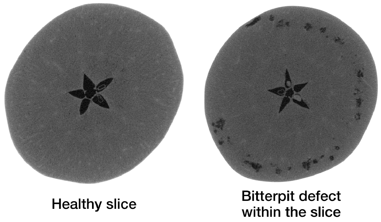
The Apple CT datasets consist of apple slices with and without internal defects. Internal defects were observed to be of four main types: bitter pit, holes, rot and browning. A reconstruction of a healthy apple slice and one with bitter pit is shown in Figure 3 as examples. Each Apple CT dataset was divided into training and test subsets using an empirical bias elimination method to ensure that apples in both subsets had similar defect statistics. This process is detailed in [38].
For the network training, the noise-free and Gaussian noise training subsets are further split into 44,647 training and 5429 validation samples, and the scattering training subset is split into 5280 training and 640 validation samples.
From the test subsets, 100 test slices were extracted in a similar manner like for the split in training and test subsets. All evaluations in this paper refer to these 100 test slices in order to keep the reconstruction time and storage volume within reasonable limits. Five slices were extracted from each of the 20 test apples such that in total each defect type is occurring with a pixel count ratio similar to its ratio on the full test subset. Additionally, the extracted slices have a pairwise distance of at least 15 slices in order to improve the image diversity. The selected list of slices is specified in the supplementing repository [39] as file supp_material/apples/test_samples_ids.csv.

3. Algorithms

A variety of learned reconstruction methods were used to create a benchmark. The selection is based on methods submitted by participants for the data challenge on the LoDoPaB-CT and Apple CT datasets. The reconstruction methods include unrolled architectures, post-processing approaches, and fully-learned methods. Furthermore, classical methods such as FBP, TV regularization and CGLS were used as a baseline.

3.1. Learned Reconstruction Methods

In this section, the learned methods included in the benchmark are presented. An overview of the hyperparameters and pseudocode can be found in Appendix A. All methods utilize artificial neural networks F Θ , each in different roles, for the reconstruction process.
Learning refers to the adaption of the parameters Θ for the reconstruction process in a data-driven manner. In general, one can divide this process into supervised and unsupervised learning. Almost all methods in this comparison are trained in a supervised way. This means that sample pairs ( y δ , x ) of noisy measurements and ground truth data are used for the optimization of the parameters, for example, by minimizing some discrepancy D X : X × X R between the output of the reconstruction model T F Θ and the ground truth
min Θ D X T F Θ y δ , x .
Supervised methods often provide excellent results, but the number of required ground truth data can be high [34]. While the acquisition of ground truth images is infeasible in many applications, this is not a problem in the low-dose and sparse-angle case. Here, reconstructions of regular (normal-dose, full-angle) scans play the role of the reference.

3.1.1. Post-Processing

Post-processing approaches aim to improve the reconstruction quality of an existing method. When used in computed tomography, FBP (cf. Appendix B.1) is often used to obtain an initial reconstruction. Depending on the scan scenario, the FBP reconstruction can be noisy or contain artifacts. Therefore, it functions as an input for a learned post-processing method. This setting simplifies the task because the post-processing network F Θ : X X maps directly from the target domain into the target domain
x ^ : = [ F Θ T FBP ] y δ .
Convolutional neural networks (CNN) have successfully been used in recent works to remove artifacts and noise from FBP reconstructions. Four of these CNN post-processing approaches were used for the benchmark. The U-Net architecture [40] is a popular choice in many different applications and was also used for CT reconstruction [20]. The details of the network used in the comparison can be found in Appendix A.2. The U-Net++  [41] (cf. Appendix A.3) and ISTA U-Net [42] (cf. Appendix A.6) represent modifications of this approach. In addition, a mixed-scale dense (MS-D)-CNN [21] is included, which has a different architecture (cf. Appendix A.4). Like for the U-Net, one can consider to adapt other architectures originally used for segmentation, for example, the ENET [43], for the post-processing task.

3.1.2. Fully Learned

The goal of fully learned methods is to extract the structure of the inversion process from data. In this case, the neural network F Θ : Y X directly maps from the measurement space Y to the target domain X. A prominent example is the AUTOMAP architecture [27], which was successfully used for reconstruction in magnetic resonance imaging (MRI). The main building blocks consist of fully-connected layers. This makes the network design very general, but the number of parameters can grow quickly with the data dimension. For example, a single fully-connected layer mapping from Y to X on the LoDoPaB-CT dataset (cf. Section 2.1) would require over 1000 × 513 × 362 2 67 × 10 9 parameters.
Adapted model designs exist for large CT data. They include knowledge about the inversion process in the structure of the network. He et al. [28] introduced an adapted two-part approach, called iRadonMap. The first part uses small fully-connected layers with parameter sharing to reproduce the structure of the FBP. This is followed by a post-processing network in the second part. Another approach is the iCT-Net [29], which uses convolutions in combination with fully-connected layers for the inversion. An extended version of the iCT-Net, called iCTU-Net, is part of our comparison and a detailed description can be found in Appendix A.8.

3.1.3. Learned Iterative Schemes

Similar to the fully learned approach, learned iterative methods also define a mapping directly from the measurement space Y to the target domain X. The idea in this case is that the network architecture is inspired by an analytic reconstruction operator T : Y X implicitly defined by an iterative scheme. The basic principle of unrolling can be explained by the example of learned gradient descent (see e.g., [17]). Let J ( · , y δ ) : X R be a smooth data discrepancy term and, possibly an additional regularization term. For an initial value x [ 0 ] the gradient descent is defined via the iteration
x [ k + 1 ] = x [ k ] ω k x J x [ k ] , y δ ,
with a step size ω k . Unrolling these iteration and stopping after K iterations, we can write the K-th iteration as
T ( y δ ) : = ( Λ ω K Λ ω 1 ) ( x [ 0 ] )
with Λ ω k : = id ω k x J · , y δ . In a learned iteration scheme, the operators Λ ω k are replaced by neural networks. As an example of a learned iterative procedure, learned primal-dual [19] was included in the comparison. A description of this method can be found in the Appendix A.1.

3.1.4. Generative Approach

The goal of the statistical approach to inverse problems is to determine the conditional distribution of the parameters given measured data. This statistical approach is often linked to Bayes’ theorem [44]. In this Bayesian approach to inverse problems, the conditional distribution p ( x | y δ ) , called the posterior distribution, is supposed to be estimated. Based on this posterior distribution, different estimators, such as the maximum a posterior solution or the conditional mean, can be used as a reconstruction for the CT image. This theory provides a natural way to model the noise behavior and to integrate prior information into the reconstruction process. There are two different approaches that have been used for CT. Adler et al. [45] use a conditional variant of a generative adversarial network (GAN, [46]) to generate samples from the posterior. In contrast to this likelihood free approach, Ardizzone et al. [47] designed a conditional variant of invertible neural networks to directly estimate the posterior distribution. These conditional invertible neural networks (CINN) were also applied to the reconstruction of CT images [48]. The CINN was included for this benchmark. For a more detailed description, see Appendix A.5.

3.1.5. Unsupervised Methods

Unsupervised reconstruction methods just make use of the noisy measurements. They are favorable in applications where ground truth data is not available. The parameters of the model are chosen based on some discrepancy D Y : Y × Y R between the output of the method and the measurements, for example,
min Θ D Y A T F Θ · , y δ .
In this example, the output of T F Θ plays the role of the reconstruction x ^ . However, comparing the distance just in the measurement domain can be problematic. This applies in particular to ill-posed reconstruction problems. For example, if the forward operator A is not bijective, no/multiple reconstruction(s) might match the measurement perfectly (ill-posed in the sense of Hadamard [49]). Another problem can occur for forward operators with an unstable inversion, where small differences in the measurement space, for example, due to noise, can result in arbitrary deviations in the reconstruction domain (ill-posed in the sense of Nashed [50]). In general, the minimization problem (6) is combined with some kind of regularization to mitigate these problems.
The optimization Formulation (6) is also used for the deep image prior (DIP) approach. DIP takes a special role among all neural network methods. The parameters are not determined on a dedicated training set, but during the reconstruction on the challenge data. This is done for each reconstruction separately. One could argue that the DIP approach is therefore not a learned method in the classical sense. The DIP approach, in combination with total variation regularization, was successfully used for CT reconstruction [34]. It is part of the comparison on the LoDoPaB dataset in this paper. A detailed description is given in Appendix A.7.

3.2. Classical Reconstruction Methods

In addition to the learned methods, we implemented the popularly used direct and iterative reconstruction methods, henceforth referred to as classical methods. They can often be described as a variational approach
T ( y δ )   arg min x D Y ( A x , y δ ) + α R ( x ) ,
where D Y : Y × Y R is a data discrepancy and R : X R is a regularizer. In this context T : Y X defines the reconstruction operator. The included methods in the benchmark are filtered back-projection (FBP) [10,51], conjugate gradient least squares (CGLS) [52,53] and anisotropic total variation minimization (TV) [54]. Detailed description of each classical method along with pseudocode are given in Appendix B.

4. Evaluation Methodology

4.1. Evaluation Metrics

Two widely used evaluation metrics were used to assess the performance of the methods.

4.1.1. Peak Signal-to-Noise Ratio

The peak signal-to-noise ratio (PSNR) is measured by a log-scaled version of the mean squared error (MSE) between the reconstruction x ^ and the ground truth image x . PSNR expresses the ratio between the maximum possible image intensity and the distorting noise
PSNR x ^ , x : = 10 log 10 L 2 MSE x ^ , x , MSE x ^ , x : = 1 n i = 1 n x ^ i x i 2 .
In general, higher PSNR values are an indication of a better reconstruction. The maximum image value L can be chosen in different ways. In our study, we report two different values that are commonly used:
  • PSNR: In this case L = max ( x ) min ( x ) , that is, the difference between the highest and lowest entry in x . This allows for a PSNR value that is adapted to the range of the current ground truth image. The disadvantage is that the PSNR is image-dependent in this case.
  • PSNR-FR: The same fixed L is chosen for all images. It is determined as the maximum entry computed over all training ground truth images, that is, L = 1.0 for LoDoPaB-CT and L = 0.0129353 for the Apple CT datasets. This can be seen as an (empirical) upper limit of the intensity range in the ground truth. In general, a fixed L is preferable because the scaling of the metric is image-independent in this case. This allows for a direct comparison of PSNR values calculated on different images. The downside for most CT applications is, that high values ( = ^ dense material) are not present in every scan. Therefore, the results can be too optimistic for these scans. However, based on Equation (7), all mean PSNR-FR values can be directly converted for another fixed choice of L.

4.1.2. Structural Similarity

The structural similarity (SSIM) [55] compares the overall image structure of ground truth and reconstruction. It is based on assumptions about the human visual perception. Results lie in the range [ 0 , 1 ] , with higher values being better. The SSIM is computed through a sliding window at M locations
SSIM x ^ , x   : = 1 M j = 1 M 2 μ ^ j μ j + C 1 2 j + C 2 μ ^ j 2 + μ j 2 + C 1 σ ^ j 2 + σ j 2 + C 2 .
In the formula above μ ^ j and μ j are the average pixel intensities, σ ^ j and σ j the variances and Σ j the covariance of x ^ and x at the j-th local window. Constants C 1 = ( K 1 L ) 2 and C 2 = ( K 2 L ) 2 stabilize the division. Following Wang et al. [55] we choose K 1 = 0.01 and K 2 = 0.03 and a window size of 7 × 7 . In accordance with the PSNR metric, results for the two different choices for L are reported as SSIM and SSIM-FR (cf. Section 4.1.1).

4.1.3. Data Discrepancy

Checking data consistency, that is, the discrepancy D Y A x ^ , y δ between the forward-projected reconstruction and the measurement, can provide additional insight into the performance of the reconstruction methods. Since noisy data is used for the comparison, an ideal method would yield a data discrepancy that is close to the present noise level.

Poisson Regression Loss on LoDoPaB-CT Dataset

For the Poisson noise model used by LoDoPaB-CT, an equivalent to the negative log-likelihood is calculated to evaluate the data consistency. It is conventional to employ the negative log-likelihood for this task, since minimizing the data discrepancy is equivalent to determining a maximum likelihood (ML) estimate (cf. Section 5.5 in [56] or Section 2.4 in [17]). Each element 𝕪 δ , j , j = 1 , , m , of a measurement 𝕪 δ , obtained according to (3) and subsequently normalized by μ max , is associated with an independent Poisson model of a photon count N ˜ 1 , j with
E ( N ˜ 1 , j ) = E N 0 exp ( 𝕪 δ , j μ max ) = N 0 exp ( y j μ max ) ,
where y j is a parameter that should be estimated [36]. A Poisson regression loss for y is obtained by summing the negative log-likelihoods for all measurement elements and omitting constant parts,
Pois ( y | y δ ) = j = 1 m N 0 exp ( y δ , j μ max ) ( y j μ max + ln ( N 0 ) ) N 0 exp ( y j μ max ) ,
with each y δ , j being the only available realization of 𝕪 δ , j . In order to evaluate the likelihood-based loss (9) for a reconstructed image x ^ given y δ , the forward projection A x ^ is passed for y.

Mean Squared Error on Apple CT Data

On the Apple CT datasets we consider the mean squared error (MSE) data discrepancy,
MSE Y ( y , y δ ) = 1 m y y δ 2 2 .
For an observation y δ with Gaussian noise (Dataset B), this data discrepancy term is natural, as it is a scaled and shifted version of the negative log-likelihood of y given y δ . In this noise setting, a good reconstruction usually should not achieve an MSE less than the variance of the Gaussian noise, that is, MSE Y ( A x ^ , y δ ) [ 0.05 1 m j = 1 m ( A x ) j ] 2 . This can be motivated intuitively by the conception that a reconstruction that achieves a smaller MSE than the expected MSE of the ground truth probably fits the noise rather than the actual data of interest.
In the setting of y δ being noise-free (Dataset A), the MSE of ideal reconstructions would be zero. On the other hand the MSE being zero does not imply that the reconstruction matches the ground truth image because of the sparse-angle setting. Further, the MSE can not be used to judge reconstruction quality directly, as crucial differences in image domain may not be equally pronounced in the sinogram domain.
For the scattering observations (Dataset C), the MSE data discrepancy is considered, too, for simplicity.

4.2. Training Procedure

While the reconstruction process with learned methods usually is efficient, their training is more resource consuming. This limits the practicability of large hyperparameter searches. It can therefore be seen as a drawback of a learned reconstruction method if they require very specific hyperparameter choices for different tasks. As a result, it benefits a fair comparison to minimize the amount of hyperparameter searches. In general, default parameters, for example, from the original publications of the respective method, were used as a starting point. For some of the methods, good choices had been determined for the LoDoPaB-CT dataset first (cf. [34]) and were kept similar for the experiments on the Apple CT datasets. Further searches were only performed if required to obtain reasonable results. More details regarding the individual methods can be found in Appendix A. For the classical methods, hyperparameters were optimized individually for each setting of the Apple CT datasets (cf. Appendix B).
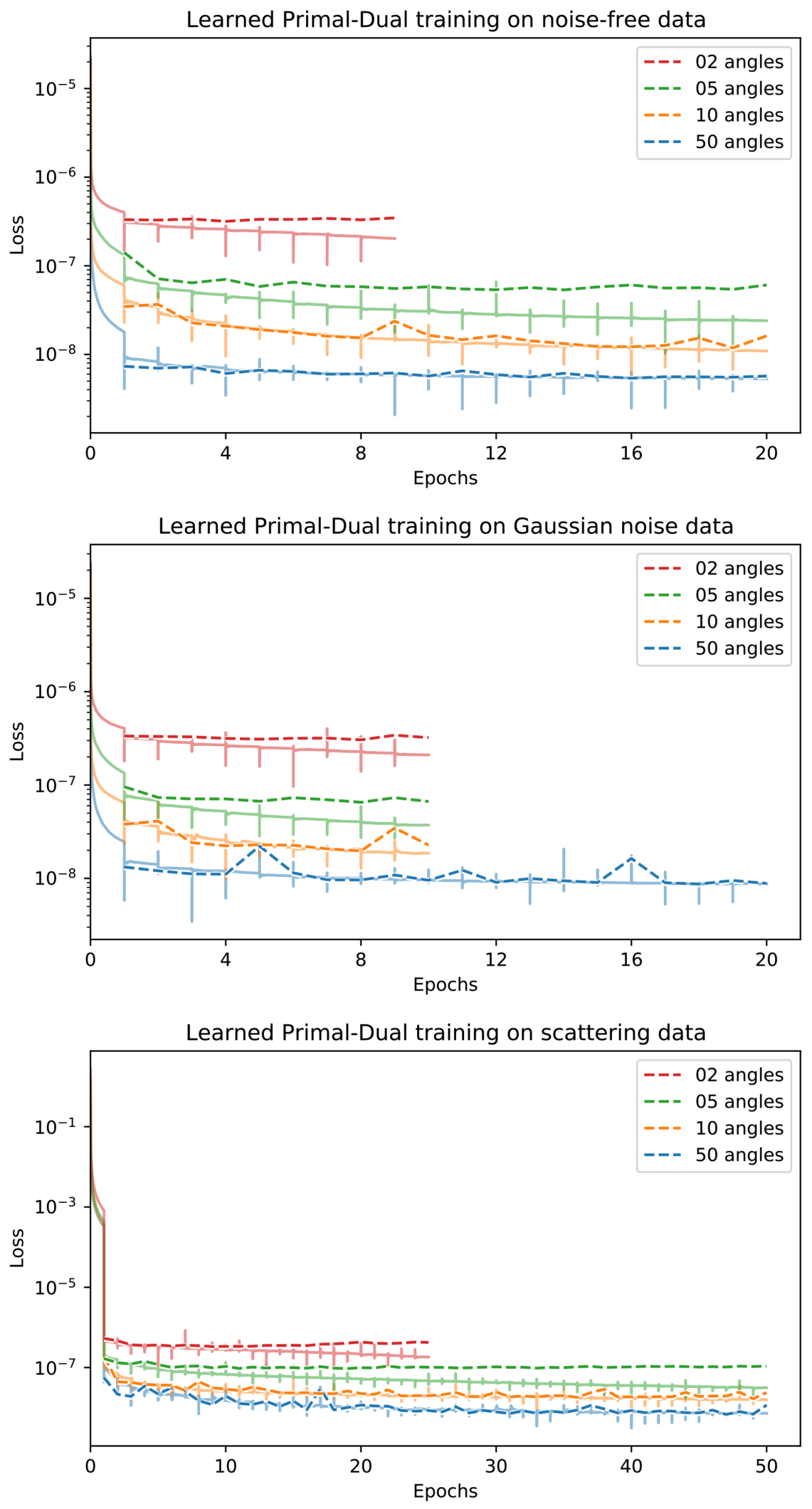
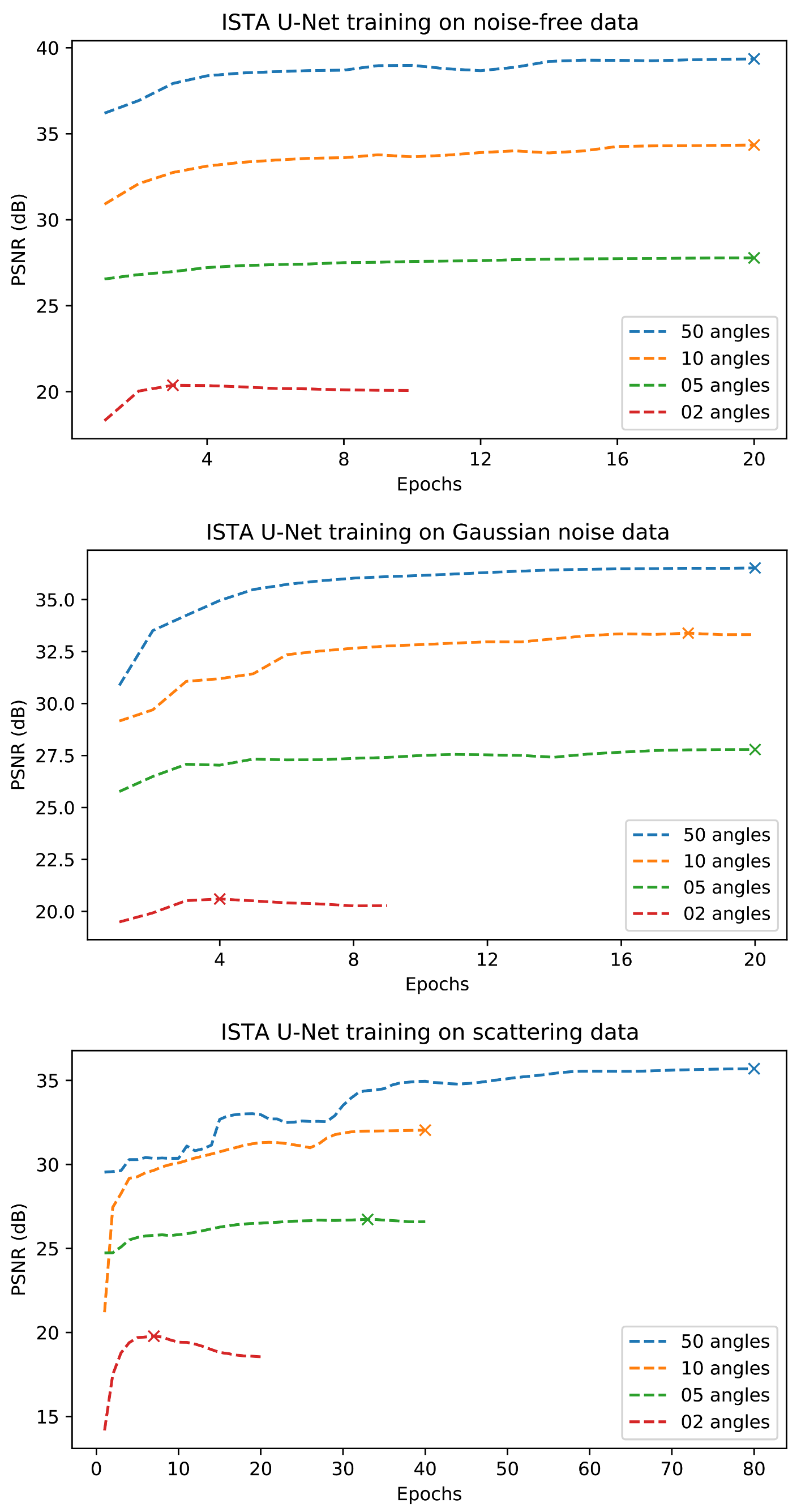
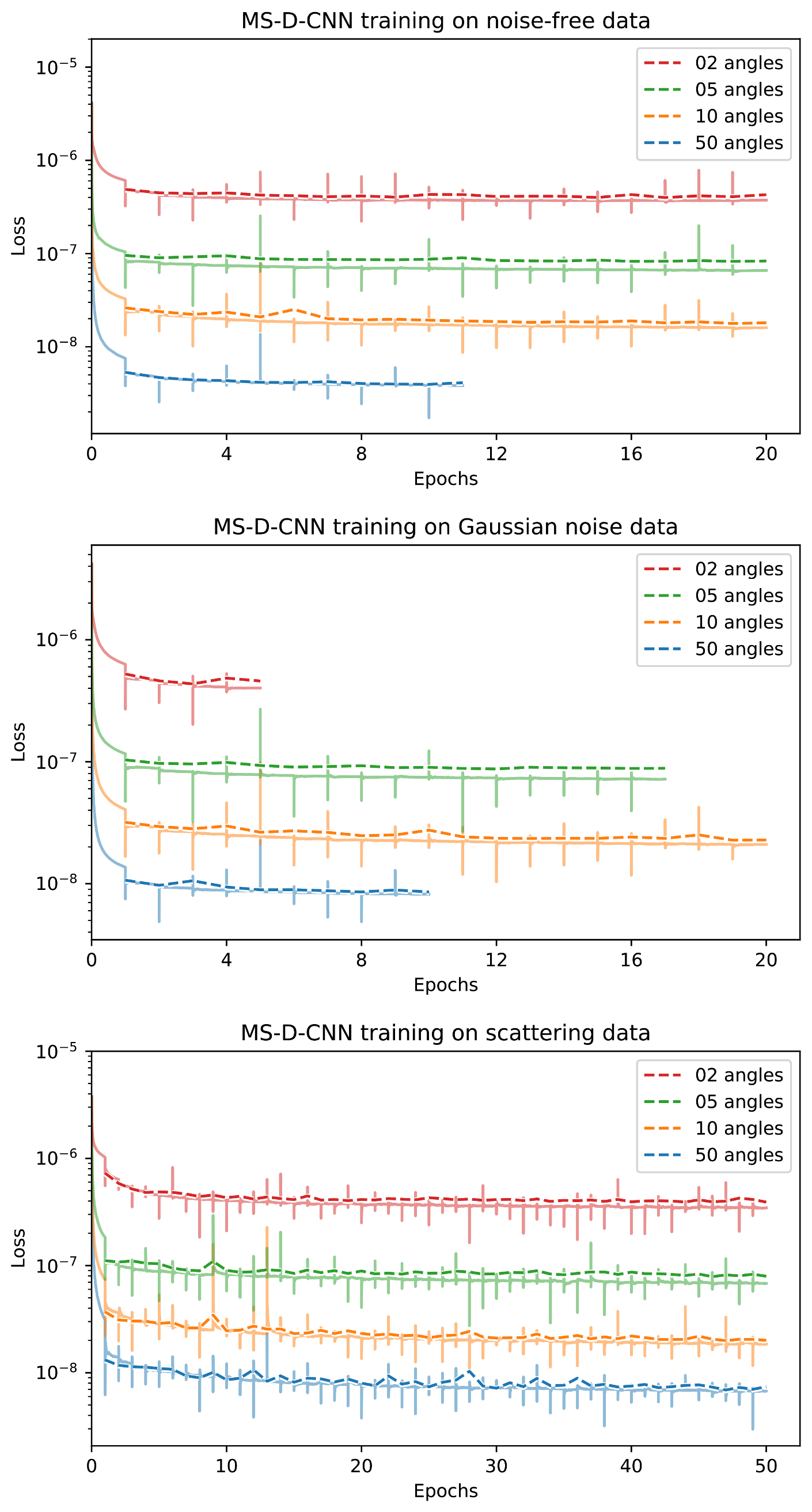
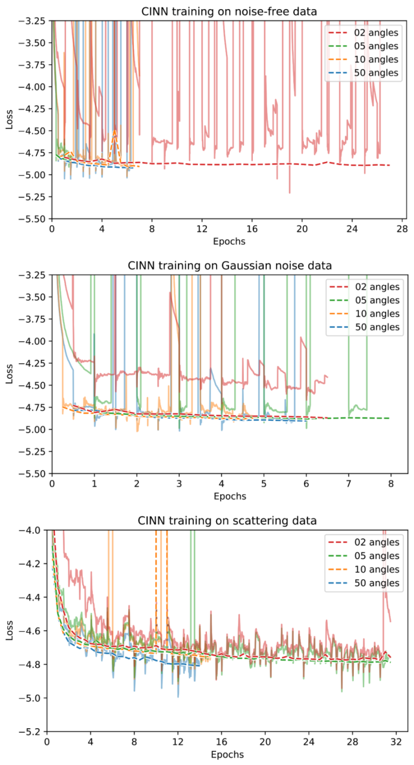
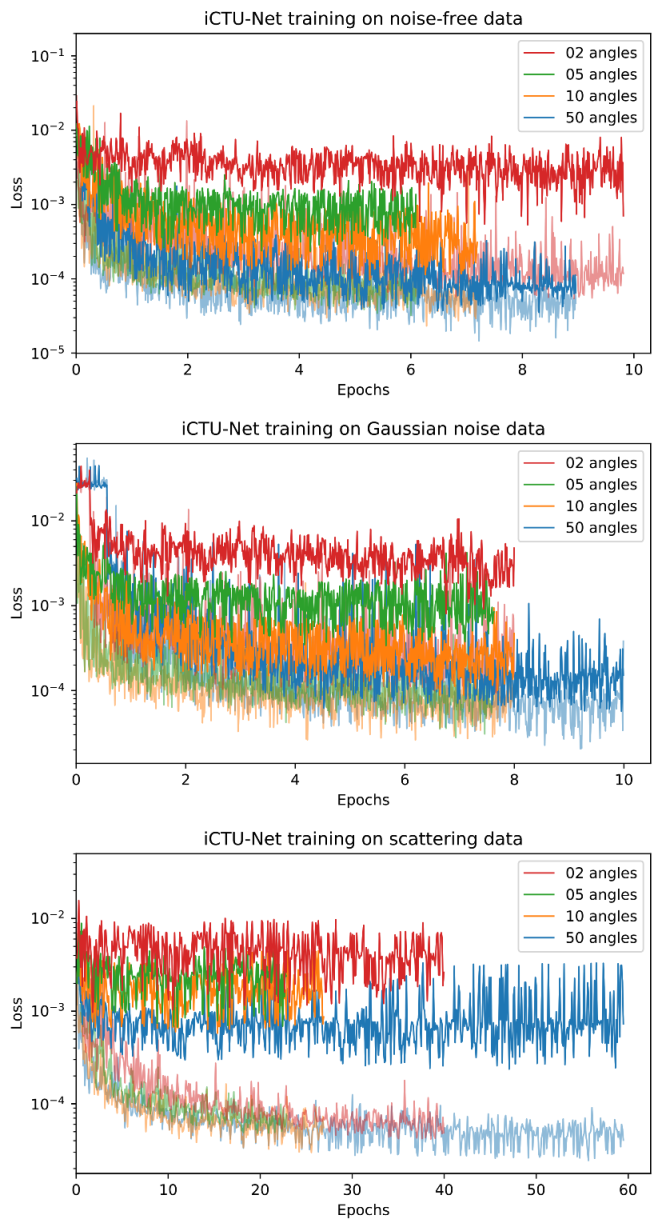
Most learned methods are trained using the mean squared error (MSE) loss. The exceptions are the U-Net++ using a loss combining MSE and SSIM, the iCTU-Net using an SSIM loss for the Apple CT datasets, and the CINN for which negative log-likelihood (NLL) and an MSE term are combined (see Appendix A for more details). Training curves for the trainings on the Apple CT datasets are shown in Appendix D. While we consider the convergence to be sufficient, continuing some of the trainings arguably would slightly improve the network. However, this mainly can be expected for those methods which are comparably time consuming to train (approximately 2 weeks for 20 epochs), in which case the limited number of epochs can be considered a fair regulation of resource usage.
Early stopping based on the validation performance is used for all trainings except for the ISTA U-Net on LoDoPaB-CT and for the iCTU-Net.
Source code is publicly available in a supplementing github repository [39]. Further records hosted by Zenodo provide the trained network parameters for the experiments on the Apple CT Datasets [57], as well as the submitted LoDoPaB-CT Challenge reconstructions [58] and the Apple CT test reconstructions of the 100 selected slices in all considered settings [59]. Source code and network parameters for some of the LoDoPaB-CT experiments are included in the DIV α library [60], for others the original authors provide public repositories containing source code and/or parameters.

5. Results

5.1. LoDoPaB-CT Dataset

Ten different reconstruction methods were evaluated on the challenge set of the LoDoPaB-CT dataset. Reconstructions from these methods were either submitted as part of the CT Code Sprint 2020 (http://dival.math.uni-bremen.de/code_sprint_2020/, last accessed: 1 March 2021) (15 June–31 August 2020) or in the period after the event (1 September–31 December 2020).

5.1.1. Reconstruction Performance

In order to assess the quality of the reconstructions, the PSNR and the SSIM were calculated. The results from the official challenge website (https://lodopab.grand-challenge.org/, last accessed: 1 March 2021) are shown in Table 2. The differences between the learned methods are generally small. Notably, learned primal-dual yields the best performance with respect to both the PSNR and the SSIM. The following places are occupied by post-processing approaches, also with only minor differences in terms of the metrics. Of the other methods, DIP + TV stands out, with relatively good results for an unsupervised method. DIP + TV is able to beat the supervised method iCTU-Net. The classical reconstruction models perform the worst of all methods. In particular, the performance of FBP shows a clear gap with the other methods. While learned primal-dual performs slightly better than the post-processing methods, the difference is not as significant as one could expect, considering that it incorporates the forward operator directly in the network. This could be explained by the beneficial combination of the convolutional architectures used for the post-processing, which are observed to perform well on a number of image processing tasks, and a sufficient number of available training samples. Otero et al. [34] investigated the influence of the size of the training dataset on the performance of different learned procedures on the LoDoPaB-CT dataset. Here, a significant difference is seen between learned primal-dual and other learned procedures when only a small subset of the training data is used.

5.1.2. Visual Comparison

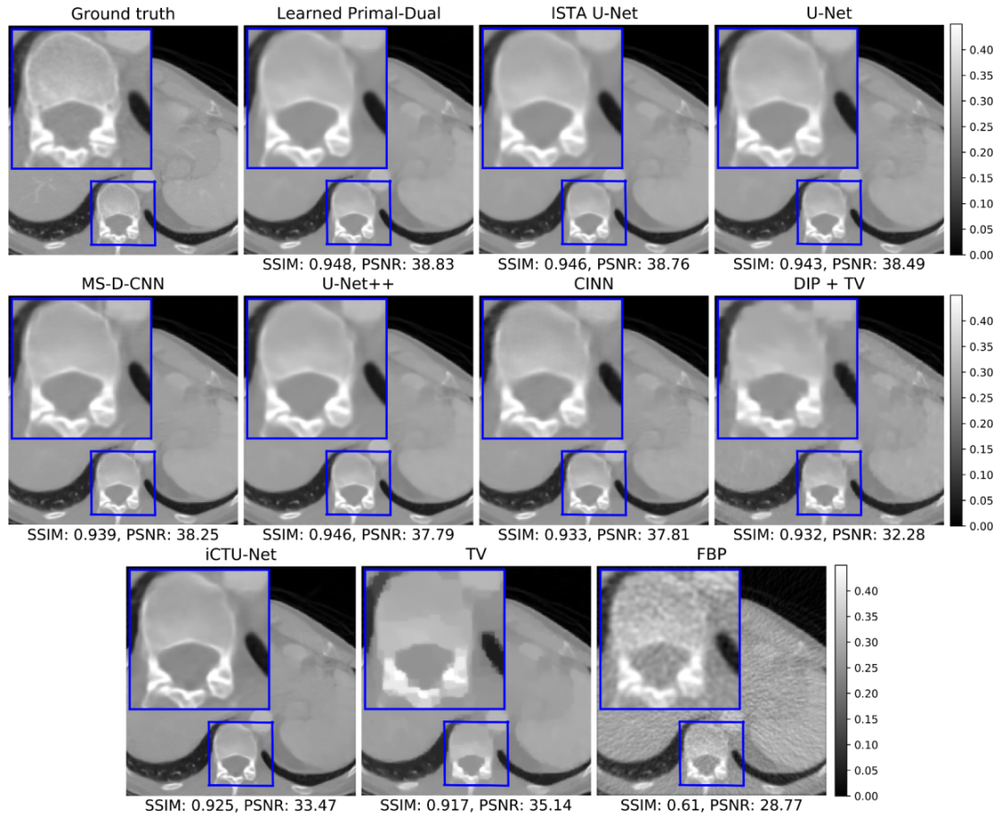
A representative reconstruction of all learned methods and the classical baseline is shown in Figure 4 to enable a qualitative comparison of the methods. An area of interest around the spine is magnified to compare the reproduction of small details and the sharpness of edges in the image. Some visual differences can be observed between the reconstructions. The learned methods produce somewhat smoother reconstructions in comparison to the ground truth. A possible explanations for the smoothness is the minimization of the empirical risk with respect to some variant of the L 2 -loss during the training of most learned methods, which has an averaging effect. The convolutional architecture of the networks can also have an impact. Adequate regularization during training and/or inference can be beneficial in this case (cf. Section 6.2.2 for a suitable class of regularizers). Additionally, the DIP + TV reconstruction appears blurry, which can be explained by the fact that it is the only unsupervised method in this comparison and thus has no access to ground truth data. The U-Net and the two modifications, U-Net++ and ISTA U-Net, show only slight visual differences on this example image.

5.1.3. Data Consistency

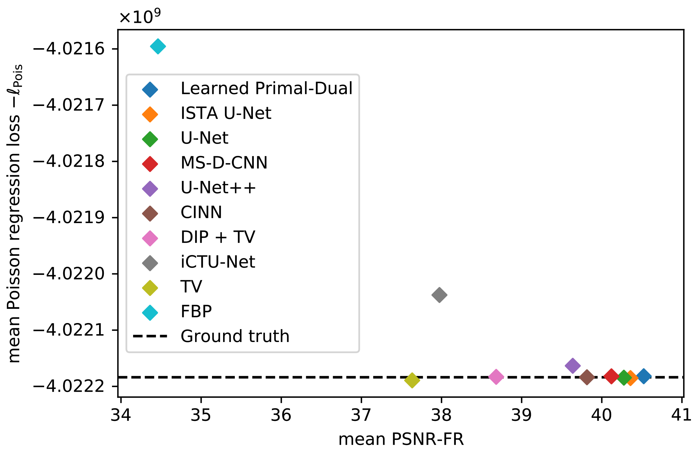
The mean data discrepancy of all methods is shown in Figure 5, plotted against their reconstruction performance. The mean difference between the noise-free and noisy measurements is included as a reference. Good-performing models should be close to this empirical noise level. Values above the mean can indicate a sub-optimal data consistency, while values below can be a sign of overfitting to the noise. A data consistency term is only explicitly used in the TV and DIP + TV model. Nevertheless, the mean data discrepancy for most of the methods is close to the empirical noise level. The only visible outliers are the FBP and the iCTU-Net. A list of all mean data discrepancy values, including standard deviations, can be found in Table 3.

5.2. Apple CT Datasets

A total of 6 different learned methods were evaluated on the Apple CT data. This set included post-processing methods (MS-D-CNN, U-Net, ISTA U-Net), learned iterative methods (learned primal-dual), fully learned approaches (iCTU-Net), and generative models (CINN). As described in Section 2.2, different noise cases (noise-free, Gaussian noise and scattering noise) and different numbers of angles (50, 10, 5, 2) were used. In total, each model was trained on the 12 different settings of the Apple CT dataset. In addition to the learned methods, three classical techniques, namely CGLS, TV, and FBP, have been included as a baseline.

5.2.1. Reconstruction Performance

A subset of 100 data samples from the test set was selected for the evaluation (cf. Section 2.2). The mean PSNR and SSIM values for all experiments can be found in Table 4. Additionally, Table A3 and Table A4, Table A5 in the appendix provide standard deviations and PSNR-FR and SSIM-FR values.
The biggest challenge with the noise-free dataset is that the measurements become increasingly undersampled as the number of angles decreases. As expected, the reconstruction quality in terms of PSNR and SSIM deteriorates significantly as the number of angles decreases. In comparison with LoDoPaB-CT, no model performs best in all scenarios. Furthermore, most methods were trained to minimize the MSE between the output image and ground truth. The MSE is directly related to the PSNR. However, minimizing the MSE does not necessarily translate into a high SSIM. In many cases, the best method in terms of PSNR does not result in the best SSIM. These observations are also evident in the two noisy datasets. Noteworthy is the performance of the classical TV method on the noise-free dataset for 50 angles. This result is comparable to the best-performing learned methods, while the other classical approaches show a clear gap.
Noisy measurements, in addition to undersampling, present an additional difficulty on the Gaussian and scattering datasets. Intuitively, one would therefore expect a worse performance compared to the noise-free case. In general, a decrease in performance can be observed. However, this effect depends on the method and the noise itself. For example, the negative impact on classical methods is much more substantial for the scattering noise. In contrast, the learned methods often perform slightly worse on the Gaussian noise. There are also some outliers with higher values than on the noise-free set. Possible explanations are the hyperparameter choices and the stochastic nature of the model training. Overall, the learned approaches can reach similar performances on the noisy data, while the performance of classical methods drops significantly. An additional observation can be made when comparing the results between Gaussian and scattering noise. For Gaussian noise with 50 angles, all learned methods, except for the iCTU net, achieve a PSNR of at least 36 dB. In contrast, the variation on scattering noise with 50 angles is much larger. The CINN obtains a much higher PSNR of 38.56 dB than the post-processing U-Net with 34.96 dB.
As already observed on the LoDoPaB dataset, the post-processing methods (MS-D-CNN, U-Net and ISTA U-Net) show only minor differences in all noise cases. This could be explained by the fact that these methods are all trained with the same objective function and differ only in their architecture.

5.2.2. Visual Comparison

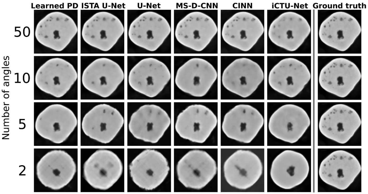
Figure 6 shows reconstructions from all learned methods for an apple slice with bitter pit. The decrease in quality with the decrease in the number of angles is clearly visible. For 2 angles, none of the methods are able to accurately recover the shape of the apple. The iCTU-Net reconstruction has sharp edges for the 2-angle case, while the other methods produce blurry reconstructions.
The inner structure, including the defects, is accurately reconstructed for 50 angles by all methods. The only exception is the iCTU-Net. Reconstructions from this network show a smooth interior of the apple. The other methods also result in the disappearance of smaller defects with fewer measurement angles. Nonetheless, a defect-detection system might still be able to sort out the apple based on the 5-angle reconstructions. The 2-angle case can be used to assess failure modes of the different approaches. The undersampling case is so severe that a lot of information is lost. However, the iCTU-Net is able to produce a smooth image of an apple, but it has few similarities with the ground truth apple. It appears that the models have memorized the roundness of an apple and produce a round apple that has little in common with the real apple except for its size and core.

5.2.3. Data Consistency

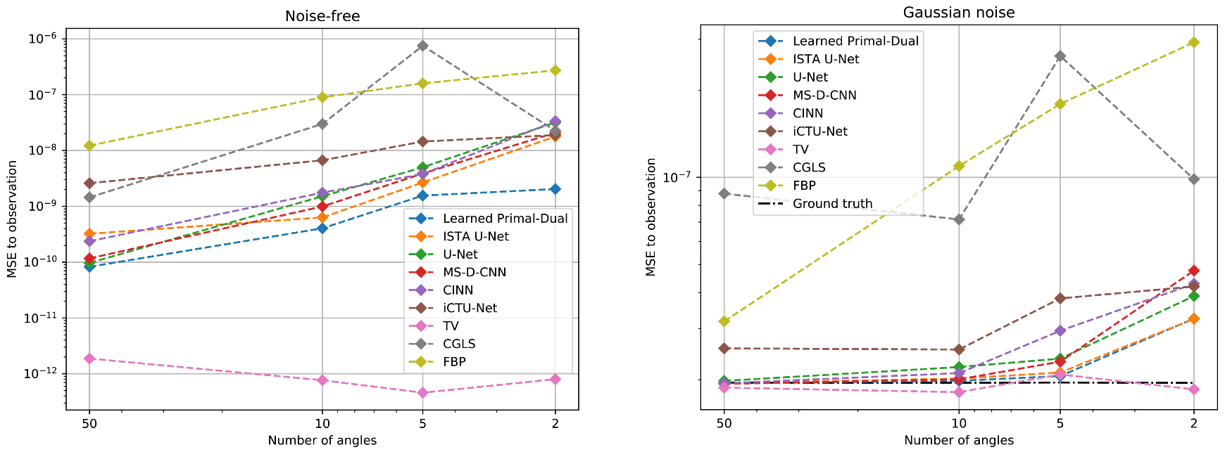
The data consistency is evaluated for all three Apple CT datasets. The MSE is used to measure the discrepancy. It is the canonical choice for measurements with Gaussian noise (cf. Section 4.1.3). Table A6 in the appendix contains all MSE values and standard deviations. Figure 7 shows the results depending on the number of angles for the noise-free and Gaussian noise dataset.
In the noise-free setup, the optimal MSE value is zero. Nonetheless, an optimal data consistency does not correspond to perfect reconstructions in this case. Due to the undersampling of the measurements, the discretized linear forward operator A has a non-trivial null space, that is, x ˜ X , apart from x ˜ = 0 , for which A x ˜ = 0 . Any element from the null space can be added to the true solution x without changing the data discrepancy
A x + x ˜ = A x + A x ˜ = A x + 0 = A x = y .
In the Gaussian setup, the MSE between noise-free and noisy measurements is used as a reference for a good data discrepancy. The problem from the undersampling is also relevant in this setting.
Both setups show an increase in the data discrepancy with fewer measurement angles. The reason for the increase is presumably the growing number of deviations in the reconstructions. In the Gaussian noise setup, the high data discrepancy of all learned methods for 2 angles coincides with the poor reconstructions of the apple slice in Figure 6. Only the TV method, which enforces data consistency during the reconstruction, keeps a constant level. The main problem for this approach are the ambiguous solutions due to the undersampling. The TV method is not able to identify the correct solution given by the ground truth. Therefore, the PSNR and SSIM values are also decreasing.
Likewise, the data consistency was analyzed for the dataset with scattering noise. The MSE values of all learned methods are close to the empirical noise level. In contrast, FBP and TV have a much smaller discrepancy. Therefore, their reconstructions are most likely influenced by the scattering noise. An effect that is also reflected in the PSNR and SSIM values in Table 4.

6. Discussion

Among all the methods we compared, there is no definite winner that is the best on both LoDoPaB-CT and Apple CT. Learned primal-dual, as an example of a learned iterative method, is the best method on LoDoPaB-CT, in terms of both PSNR and SSIM, and also gives promising results on Apple CT. However, it should be noted that the differences in performance between the learned methods are relatively small. The ISTA U-Net, second place in terms of PSNR on LoDoPaB-CT, scores only 0.14 dB less than learned primal-dual. The performance in terms of SSIM is even closer on LoDoPaB-CT. The best performing learned method resulted in an SSIM that was only 0.022 higher than the last placed learned method. The observation that the top scoring learned methods did not differ greatly in terms of performance has also been noted in the fastMRI challenge [61]. In addition to the performance of the learned methods, other characteristics are also of interest.

6.1. Computational Requirements and Reconstruction Speed

When discussing the computational requirements of deep learning methods, it is important to distinguish between training and inference. Training usually requires significantly more processing power and memory. All outputs of intermediate layers have to be stored for the determination of the gradients during backpropagation. Inference is much faster and less resource-intensive. In both cases, the requirements are directly influenced by image size, network architecture and batch size.
A key feature and advantage of the learned iterative methods, post-processing methods and fully-learned approaches is the speed of reconstruction. Once the network is trained, the reconstruction can be obtained by a simple forward pass of the model. Since the CINN, being a generative model, draws samples from the posterior distribution, many forward passes are necessary to well approximate the mean or other moments. Therefore, the quality of the reconstruction may depend on the number of forward passes [48]. The DIP + TV method requires a separate model to be trained to obtain a reconstruction. As a result, reconstruction is very time-consuming and resource-intensive, especially on the 972   p x × 972   p x images in the Apple CT datasets. However, DIP + TV does not rely on a large, well-curated dataset of ground truth images and measurements. As an unsupervised method, only measurement data is necessary. The large size of the Apple CT images is also an issue for the other methods. In comparison to LoDoPaB-CT, the batch size had to be reduced significantly in order to train the learned models. This small batch size can cause instability in the training process, especially for CINN (cf. Figure A14).

Transfer to 3D Reconstruction

The reconstruction methods included in this study were evaluated based on the reconstruction of individual 2D slices. In real applications, however, the goal is often to obtain a 3D reconstruction of the volume. This can be realized with separate reconstructions of 2D slices, but (learned) methods might benefit from additional spatial information. On the other hand, a direct 3D reconstruction can have a high demand on the required computing power. This is especially valid when training neural networks.
One way to significantly reduce the memory consumption of backpropagation is to use invertible neural networks (INN). Due to the invertibility, the intermediate activations can be calculated directly and do not have to be stored in memory. INNs were successfully applied to 3D reconstructions tasks in MRI [62] and CT [63]. The CINN approach from our comparison can be adapted in a similar way for 3D data. In most post-processing methods, the U-Net can be replaced by an invertible iUnet, as proposed by Etmann et al. [63].
Another option is the simultaneous reconstruction of only a part of the volume. The information from multiple neighboring slices is used in this case, which is also referred to as 2.5D reconstruction. Networks that operate on this scenario usually have a mixture of 2D and 3D convolutional layers [64]. The goal is to strike a balance between the speed and memory advantage of the 2D scenario and the additional information from the third dimension. All deep learning methods included in this study would be suitable for 2.5D reconstruction with slight modifications to their network architecture.
Overall, 2.5D reconstruction can be seen as an intermediate step that can already be realized with many learned methods. The pure 3D case, on the other hand, requires specially adapted deep learning approaches. Technical innovations such as mixed floating point precision and increasing computing power may facilitate the transition in the coming years.

6.2. Impact of the Datasets

The type, composition and size of a dataset can have direct impact on the performance of the models. The observed effects can provide insight into how the models can be improved or how the results translate to other datasets.

6.2.1. Number of Training Samples

A large dataset is often required to successfully train deep learning methods. In order to assess the impact of the number of data pairs on the performance of the methods, we consider the Apple CT datasets. The scattering noise dataset (Dataset C), with 5280 training images, is only about 10% as large as the noise free dataset (Dataset A) and the Gaussian noise dataset (Dataset B). Here it can be noted that the iCTU net, as an example of a fully learned approach, performs significantly worse on this smaller dataset than on dataset A and dataset B ( 26.26 dB PSNR on Dataset C with 50 angles, 36.07 dB and 32.90 dB on Dataset A and Dataset B with 50 angles, respectively). This drop in performance could also be caused by the noise case. However, Baguer et al. [34] have already noted in their work that the performance of fully learned approaches heavily depends on the number of training images. This could be explained by the fact that fully learned methods need to infer most of the information about the inversion process purely from data. Unlike learned iterative methods, such as learned primal-dual, fully learned approaches do not incorporate the physical model. A drop in performance due to a smaller training set was not observed for the other learned methods. However, 5280 training images is still comprehensive. Baguer et al. [34] also investigated the low-data regime on LoDoPaB-CT, down to around 30 training samples. In their experiments, learned primal-dual worked well in this scenario, but was surpassed by the DIP + TV approach. The U-Net post-processing lined up between learned Primal-Dual and the fully learned method. Therefore, the amount of available training data should be considered when choosing a model. To enlarge the training set, the DIP + TV approach can also be used to generate pseudo ground truth data. Afterwards, a supervised method with a fast reconstruction speed can be trained to mimic the behavior of DIP + TV.

6.2.2. Observations on LoDoPaB-CT and Apple CT

The samples and CT setups differ greatly between the two datasets. The reconstructions obtained using the methods compared in this study reflect these differences to some extent, but there were also some effects that were observed for both datasets.
The sample reconstructions in Figure 4 and Figure 6 show that most learned methods produce smooth images. The same observation can be made for TV, where smoothness is an integral part of the modeling. An extension by a suitable regularization can help to preserve edges in the reconstruction without the loss of small details, or the introduction of additional noise. One possibility is to use diffusion filtering [65], for example, variants of the Perona-Malik diffusion [66] in this role. Diffusion filtering was also successfully applied as a post-processing step for CT [67]. Whether smoothness of reconstructions is desired depends on the application and further use of the images, for example, visual or computer-aided diagnosis, screening, treatment planning, or abnormality detection. For the apple scans, a subsequent task could be the detection of internal defects for sorting them into different grades. The quality of the reconstructions deteriorates with the decreasing number of measurement angles. Due to increasing undersampling, the methods have to interpolate more and more information to find an adequate solution. The model output is thereby influenced by the training dataset.
The effects of severe undersampling can be observed in the 2-angle setup in Figure 6. All reconstructions of the test sample show a prototypical apple with a round shape and a core in the center. The internal defects are not reproduced. One explanation is that supervised training aims to minimize the empirical risk on the ground truth images. Therefore, only memorizing and reconstructing common features in the dataset, like the roundness and the core, can be optimal in some ways to minimize the empirical risk on severely undersampled training data. Abnormalities in the data, such as internal defects, are not captured in this case. This effect is subsequently transferred to the reconstruction of test data. Hence, special attention should be paid to the composition of the training data. As shown in the next Section 6.2.3, this is particularly important when the specific features of interest are not well represented in the training set.
In the 5-angle setup, all methods are able to accurately reconstruct the shape of the apple. Internal defects are partially recovered only by the post-processing methods and the CINN. These approaches all use FBP reconstructions as a starting point. Therefore, they rely on the information that is extracted by the FBP. This can be useful in the case of defects but aggravating for artifacts in the FBP reconstruction. The CINN approach has the advantage of sampling from the space of possible solutions and the evaluability of the likelihood under the model. This information can help to decide whether objects in the reconstruction are really present.
In contrast, Learned Primal-Dual and the iCTU-Net work directly on the measurements. They are more flexible with respect to the extraction of information. However, this also means that the training objective strongly influences which aspects of the measurements are important for the model. Tweaking the objective or combining the training of a reconstruction and a detection model, that is, end-to-end learning or task-driven reconstruction, might be able to increase the model performance in certain applications [68,69].

6.2.3. Robustness to Changes in the Scanning Setup

A known attribute of learned methods is that they can often only be applied to data similar to the training data. It is often unclear how a method trained in one setting generalizes to a different setting. In CT, such a situation could for example arise due to altered scan acquisition settings or application to other body regions. Switching between CT devices from different manufacturers can also have an impact.
As an example, we evaluated the U-Net on a different number of angles than it was trained on. The results of this experiment are shown in Table 5. In most setups the PSNR drops by at least 10 dB when evaluated on a different setting. In practice, the angular sampling pattern may change and it would be cumbersome to train a separate model for each pattern.

6.2.4. Generalization to Other CT Setups

The LoDoPaB-CT and Apple CT datasets were acquired by simulating parallel-beam measurements, based on the Radon transform. This setup facilitates large-scale experiments with many example images, whereas the underlying operators in the algorithms have straightforward generalizations to other geometries. Real-world applications of CT are typically more complex. For example, the standard scanning geometries in medical applications are helical fan-beam or cone-beam [36]. In addition, the simulation model does not cover all physical effects that may occur during scanning. For this reason, the results can only be indicative of performance on real data.
However, learned methods are known to adapt well to other setups when retrained from scratch on new samples. It is often not necessary to adjust the architecture for this purpose, other than by replacing the forward operator and its adjoint where they are involved. For example, most learned methods show good performance on the scattering observations, whereas the classical methods perform worse compared to the Gaussian noise setup. This can be explained by the fact that the effect of scattering is structured, which, although adding to the instability of the reconstruction problem, can be learned to be (partially) compensated for. In contrast, classical methods require the reconstruction model to be manually adjusted in order to incorporate knowledge about the scattering. If scattering is treated like an unknown distortion (i.e., a kind of noise), such as in our comparison, the classical assumption of pixel-wise independence of the noise is violated by the non-local structure of the scattering. Convolutional neural networks are able to capture these non-local effects.

6.3. Conformance of Image Quality Scores and Requirements in Real Applications

The goal in tomographic imaging is to provide the expert with adequate information through a clearly interpretable reconstructed image. In a medical setting, this can be an accurate diagnosis or plan for an operation; and in an industrial setting, the image may be used for detection and identification of faults or defects as part of quality control.
PSNR and SSIM, among other image quality metrics, are commonly used in publications and data challenges [61] to evaluate the quality of reconstructed medical images [70]. However, there can be cases in which PSNR and SSIM are in a disagreement. Although not a huge difference, the results given in Table 4 are a good example of this. This often leads to the discussion of which metric is better suited for a certain application. The PSNR expresses a pixel-wise difference between the reconstructed image and its ground truth, whereas the SSIM checks for local structural similarities (cf. Section 4.1). A common issue with both metrics is that a local inaccuracy in the reconstructed image, such as a small artifact, would only have a minor influence on the final assessment. The effect of the artifact is further downplayed when the PSNR or SSIM values are averaged over the test samples. This is evident in some reconstructions from the DIP + TV approach, where an artifact was observed on multiple LoDoPaB-CT reconstructions whereas this is not reflected in the metrics. This artifact is highlighted with a red circle in the DIP + TV reconstruction in Figure A2.
An alternative or supporting metric to PSNR and SSIM is visual inspection of the reconstructions. A visual evaluation can be done, for example, through a blind study with assessments and rating of reconstructions by (medical) experts. However, due to the large amount of work involved, the scope of such an evaluation is often limited. The 2016 Low Dose CT Grand Challenge [9] based their comparison on the visibility of liver lesions, as evaluated by a group of physicians. Each physician had to rate 20 different cases. The fastMRI Challenge [61] employed radiologists to rank MRI reconstructions. The authors were able to draw parallels between the quantitative and blind study results, which revealed that, in their data challenge, SSIM was a reasonable estimate for the radiologists’ ranking of the images. In contrast, Mason et al. [71] found differences in their study between several image metrics and experts’ opinions on reconstructed MRI images.
In industrial settings, PSNR or related pixel-based image quality metrics fall short on assessing the accuracy or performance of a reconstruction method when physical and hardware-related factors in data acquisition play a role in the final reconstruction. These factors are not accurately reflected in the image quality metrics, and therefore the conclusions drawn may not always be applicable. An alternative practice is suggested in [72], in which reconstructions of a pack of glass beads are evaluated using pixel-based metrics, such as contrast-to-noise ratio (CNR), and pre-determined physical quantification techniques. The physical quantification is object-specific, and assessment is done by extracting a physical quality of the object and comparing this to a reference size or shape. In one of the case studies, the CNR values of iterated reconstructions suggest an earlier stopping for the best contrast in the image, whereas a visual inspection reveals the image with the “best contrast” to be too blurry and the bead un-segmentable. The Apple CT reconstructions can be assessed in a similar fashion, where we look at the overall shape of a healthy apple, as well as the shape and position of its pit.

6.4. Impact of Data Consistency

Checking the discrepancy between measurement and forward-projected reconstruction can provide additional insight into the quality of the reconstruction. Ground truth data is not needed in this case. However, an accurate model A of the measurement process must be known. Additionally, the evaluation must take into account the noise type and level, as well as the sampling ratio.
Out of all tested methods, only the TV, CGLS and DIP + TV approach use the discrepancy to the measurements as (part of) their minimization objective for the reconstruction process. Still, the experiments on LoDoPaB-CT and Apple CT showed data consistency on the test samples for most of the methods. Based on these observations, data consistency does not appear to be a problem with test samples coming from a comparable distribution to the training data. However, altering the scan setup can significantly reduce the reconstruction performance of learned methods (cf. Section 6.2.3). Verification of the data consistency can serve as an indicator without the need for ground truth data or continuous visual inspection.
Another problem can be the instability of some learned methods, which is also known under the generic term of adversarial attacks [73]. Recent works [74,75] show that some methods, for example, fully learned and post-processing approaches, can be unstable. Tiny perturbations in the measurements may result in severe artifacts in the reconstructions. Checking the data discrepancy may also help in this case. Nonetheless, severe artifacts were also found in some reconstructions from the DIP + TV method on LoDoPaB-CT.
All in all, including a data consistency objective in training (bi-directional loss), could further improve the results from learned approaches. Checking the discrepancy during the application of trained models can also provide additional confidence about the reconstructions’ accuracy.

6.5. Recommendations and Future Work

As many learned methods demonstrated similar performance in both low-dose CT and sparse-angle CT setups, further attributes have to be considered when selecting a learned method for a specific application. As discussed above, consideration should also be given to reconstruction speed, availability of training data, knowledge of the physical process, data consistency, and subsequent image analysis tasks. An overview can be found in Table 6. From the results of our comparison, some recommendations for the choice and further investigation of deep learning methods for CT reconstruction emerge.
Overall, the learned primal-dual approach proved to be a solid choice on the tested low photon count and sparse-angle datasets. The applicability of the method depends on the availability and fast evaluation of the forward and the adjoint operators. Both requirements were met for the 2D parallel beam simulation setup considered. However, without adjustments to the architecture, more complicated measurement procedures and especially 3D reconstruction could prove challenging. In contrast, the post-processing methods are more flexible, as they only rely on some (fast) initial reconstruction method. The performance of the included post-processing models was comparable to learned primal-dual. A disadvantage is the dependence on the information provided by the initial reconstruction.
The other methods included in this study are best suited for specific applications due to their characteristics. Fully learned methods do not require knowledge about the forward operator, but the necessary amount of training data is not available in many cases. The DIP + TV approach is on the other side of the spectrum, as it does not need any ground truth data. One downside is the slow reconstruction speed. However, faster reconstruction methods can be trained based on pseudo ground truth data created by DIP + TV. The CINN method allows for the evaluation of the likelihood of a reconstruction and can provide additional statistics from the sampling process. The invertible network architecture also enables the model to be trained in a memory-efficient way. The observed performance for 1000 samples per reconstruction was comparable to the post-processing methods. For time-critical applications, the number of samples would need to be lowered considerably, which can deteriorate the image quality.
In addition to the choice of model, the composition and amount of the training data also plays a significant role for supervised deep learning methods. The general difficulty of application to data that deviate from the training scenario was also observed in our comparison. Therefore, the training set should either contain examples of all expected cases or the model must be modified to include guarantees to work in divergent scenarios, such as different noise levels or number of angles. Special attention should also be directed to subsequent tasks. Adjusting the training objective or combining training with successive detection models can further increase the value of the reconstruction. Additionally, incorporating checks for the data consistency during training and/or reconstruction can help to detect and potentially prevent deviations in reconstruction quality. This potential is currently underutilized by many methods and could be a future improvement. Furthermore, the potential of additional regularization techniques to reduce the smoothness of reconstructions from learned methods should be investigated.
Our comparison lays the foundation for further research that is closer to real-world applications. Important points are the refinement of the simulation model, the use of real measurement data and the transition to fan-beam/cone-beam geometries. The move to 3D reconstruction techniques and the study of the influence of the additional spatial information is also an interesting aspect. Besides the refinement of the low photon count and sparse-angle setup, a future comparison should include limited-angle CT. A first application of this setting to Apple CT can be found in the dataset descriptor [38].
An important aspect of the comparison was the use of PSNR and SSIM image quality metrics to rate the produced reconstructions. In the future, this assessment should be supplemented by an additional evaluation of the reconstruction quality of some samples by (medical) professionals. A multi-stage blind study for the evaluation of unmarked reconstructions, including or excluding the (un)marked ground truth image, may provide additional insights.
Finally, a comparison is directly influenced by the selection of the included models. While we tested a broad range of different methods, there are still many missing types, for example, learned regularization [18] and null space networks [76]. We encourage readers to test additional reconstruction methods on the datasets from our comparison and submit reconstructions to the respective data challenge websites: (https://lodopab.grand-challenge.org/, last accessed: 1 March 2021) and (https://apples-ct.grand-challenge.org/, last accessed: 1 March 2021).

7. Conclusions

The goal of this work is to quantitatively compare learned, data-driven methods for image reconstruction. For this purpose, we organized two online data challenges, including a 10-day kick-off event, to give experts in this field the opportunity to benchmark their methods. In addition to this event, we evaluated some popular learned models independently. The appendix includes a thorough explanation and references to the methods used. We focused on two important applications of CT. With the LoDoPaB-CT dataset we simulated low-dose measurements and with the Apple CT datasets we included several sparse-angle setups. In order to ensure reproducibility, the source code of the methods, network parameters and the individual reconstruction are released. In comparison to the classical baseline (FBP and TV regularization) the data-driven methods are able to improve the quality of the CT reconstruction in both sparse-angle and low-dose settings. We observe that the top scoring methods, namely learned primal-dual and different post-processing approaches, perform similarly well in a variety of settings. Besides that, the applicability of deep learning-based models depends on the availability of training examples, prior knowledge about the physical system and requirements for the reconstruction speed.

Supplementary Materials

Author Contributions

Conceptualization, J.L., M.S., P.S.G., P.M. and M.v.E.; Data curation, J.L., V.A. and S.B.C.; Formal analysis, J.L., M.S., P.S.G., V.A., S.B.C. and A.D.; Funding acquisition, K.J.B. and P.M.; Investigation, J.L., M.S., V.A., S.B.C. and A.D.; Project administration, M.S.; Software, J.L., M.S., P.S.G., V.A., S.B.C., A.D., D.B., A.H. and M.v.E.; Supervision, K.J.B., P.M. and M.v.E.; Validation, J.L. and M.S.; Visualization, J.L. and A.D.; Writing—original draft, J.L., M.S., P.S.G., V.A., S.B.C., A.D., D.B., A.H. and M.v.E.; Writing—review & editing, J.L., M.S., P.S.G., V.A., S.B.C., A.D., D.B., A.H., K.J.B., P.M. and M.v.E. All authors have read and agreed to the published version of the manuscript.

Funding

J.L., M.S., A.D. and P.M. were funded by the German Research Foundation (DFG; GRK 2224/1). J.L. and M.S. additionally acknowledge support by the project DELETO funded by the Federal Ministry of Education and Research (BMBF, project number 05M20LBB). A.D. further acknowledges support by the Klaus Tschira Stiftung via the project MALDISTAR (project number 00.010.2019). P.S.G. was funded by The Marie Skłodowska-Curie Innovative Training Network MUMMERING (Grant Agreement No. 765604). S.B.C. was funded by The Netherlands Organisation for Scientific Research (NWO; project number 639.073.506). M.v.E. and K.J.B. acknowledge the financial support by Holland High Tech through the PPP allowance for research and development in the HTSM topsector.

Institutional Review Board Statement

Not applicable.

Informed Consent Statement

Not applicable.

Data Availability Statement

The two datasets used in this study are the LoDoPaB-CT dataset [32], and the AppleCT dataset [37], both publicly available on Zenodo. The reconstructions discussed in Section 5 are provided as supplementary materials to this submission. These are shared via Zenodo through [57,58,59].

Acknowledgments

We are grateful for the help of GREEFA b.v. and the FleX-ray Laboratory of CWI for making CT scans of apples with internal defects available for the Code Sprint. The Code Sprint was supported by the DFG and the European Commission’s MUMMERING ITN. We would like to thank Jens Behrmann for fruitful discussions. Finally, we would like to thank all participants of the Code Sprint 2020 for contributing to the general ideas and algorithms discussed in this paper.

Conflicts of Interest

The authors declare no conflict of interest, financial or otherwise.

Appendix A. Learned Reconstruction Methods

Appendix A.1. Learned Primal-Dual

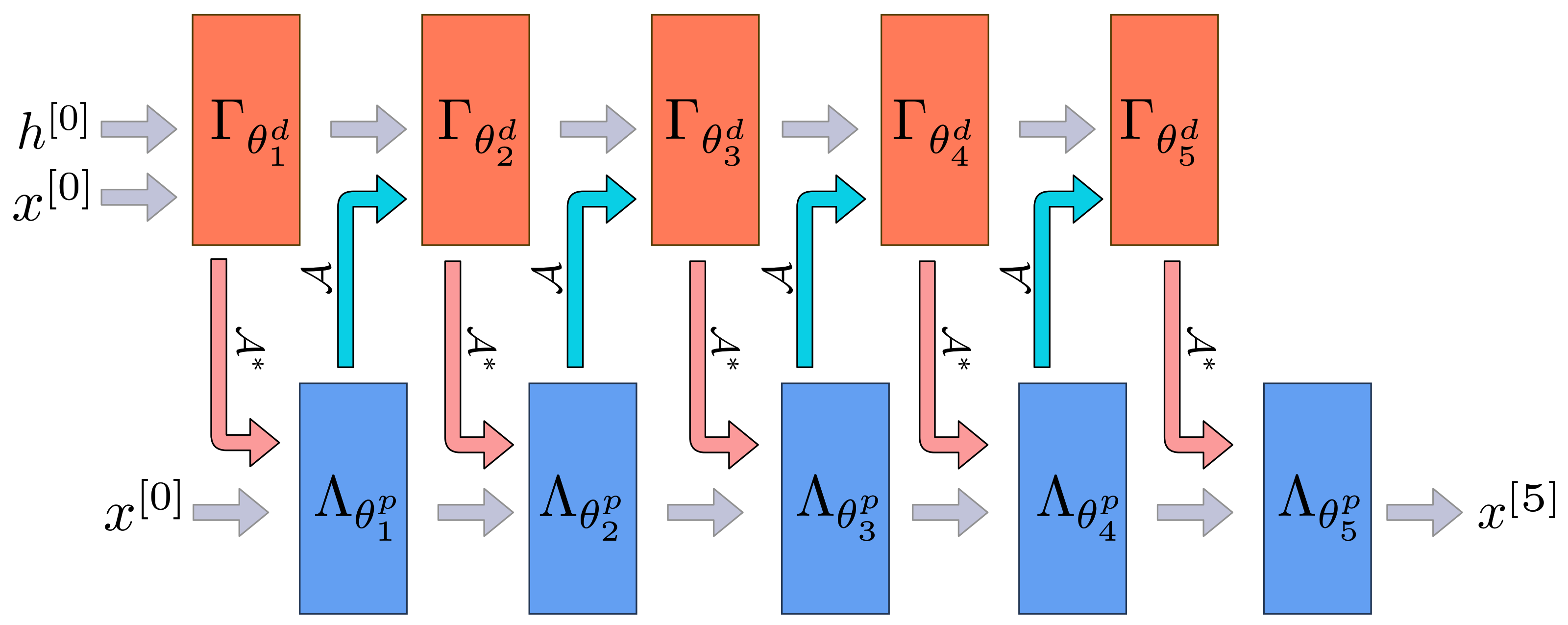
The Learned Primal-Dual algorithm is a learned iterative procedure to solve inverse problems [19]. A primal-dual scheme [77] is unrolled for a fixed number of steps and the proximal operators are replaced by neural networks (cf. Figure A1). This unrolled architecture is then trained using data pairs from measurements and ground truth reconstructions. The forward pass is given in Algorithm A1. In contrast to the regular primal-dual algorithm, the primal and the dual space are extended to allow memory between iterations:
x = [ x ( 1 ) , , x ( N primal ) ] X N primal , h = [ h ( 1 ) , , h ( N dual ) ] Y N dual .
For the benchmark N primal = 5 and N dual = 5 was used. Both the primal and dual operators were parameterized as convolutional neural networks with 3 layers and 64 intermediate convolution channels. The primal-dual algorithm was unrolled for K = 10 iterations. Training was performed by minimizing the mean squared error loss using the Adam optimizer [78] with a learning rate of 0.0001 . The model was trained for 10 epochs on LoDoPaB-CT and for at most 50 epochs on the apple data, whereby the model with the highest PSNR on the validation set was selected. Batch size 1 was used. Given a learned primal-dual algorithm the reconstruction can be obtained using Algorithm A1.
Algorithm A1 Learned Primal-Dual.
Given learned proximal dual and primal operators Γ θ k d , Λ θ k p for k = 1 , , K the reconstruction from noisy measurements y δ is calculated as follows.
1.
   Initialize x [ 0 ] X N primal , h [ 0 ] Y N dual
2.
   for   k = 1 : K
3.
     h [ k ] = Γ θ k d h [ k 1 ] , A ( x ( 2 ) [ k 1 ] ) , y δ
4.
     x [ k ] = Λ θ k p x [ k 1 ] , A ( x ( 1 ) [ k 1 ] ) * ( h ( 1 ) [ m ] )
5.
   end
6.
   return  x ^ = x ( 1 ) [ K ]
Figure A1. Architecture of the learned primal dual algorithm unrolled for K = 5 iterations. We used a zero initialization for h [ 0 ] and the FBP reconstruction for x [ 0 ] . Adapted from [19].
Jimaging 07 00044 g0a1

Appendix A.2. U-Net

The goal of post-processing methods is to improve a pre-computed reconstruction. For CT, the FBP is used to obtain an initial reconstruction. This reconstruction is then used as an input to a post-processing network. For the enhancement of CT reconstructions, the post-processing network is implemented as a U-Net [20]. The U-Net architecture, as proposed by Ronneberger et al. [40], was originally designed for the task of semantic segmentation, but has many properties that are also beneficial for denoising. The general architecture is shown in Figure A2. In our implementation we used 5 scales (4 up- and downsampling blocks each) both for the LoDoPaB-CT and the Apple CT datasets. The skip connection between same scale levels mitigates the vanishing gradient problem so that deeper networks can be trained. In addition, the multi-scale architecture can be considered as a decomposition of the input image, in which an optimal filtering can be learned for each scale. There are many extensions to this basic architecture. For example, the U-Net++ (cf. Appendix A.3) extends the skip connections to different pathways.
The used numbers of channels at the different scales are 32, 32, 64, 64, and 128. For all skip connections 4 channels were used. The input FBPs were computed with Hann filtering and no frequency scaling. Linear activation (i.e., no sigmoid or ReLU activation) was used for the network output. Training was performed by minimizing the mean squared error loss using the Adam optimizer. For each training, the model with the highest PSNR on the validation set was selected. Due to the different memory requirements imposed by the image sizes of LoDoPaB-CT and the Apple CT data, different batch sizes were used. While for LoDoPaB-CT the batch size was 32 and standard batch normalization was applied, for the Apple CT data a batch size of 4 was used and layer normalization was applied instead of batch normalization. On LoDoPaB-CT, the model was trained for 250 epochs with learning rate starting from 0.001, reduced to 0.0001 by cosine annealing. On the Apple CT datasets, the model was trained for at most 50 epochs with fixed learning rate 0.001.
Figure A2. Architecture of the mutli-scale, post-processing U-Net. The general architecture of a U-Net consists on a downsampling path on the left and a upsampling path on the right with intermediate connection between similar scales. Adapted from [40].
Jimaging 07 00044 g0a2

Appendix A.3. U-Net++

The U-Net++ was introduced by Zhou et al. [41], the network improves on the original U-Net [40] architecture by incorporating nested and dense convolution blocks between skip connections. In U-Net, the down-sample block outputs of the encoder are directly input into the decoder’s up-sample block at the same resolution. In U-Net++, the up-sampling block receives a concatenated input of a series of dense convolutional blocks at the same resolution. The input to these dense convolutional blocks is the concatenation of all previous dense convolutional blocks and the corresponding up-sample of a lower convolutional block.
The design is intended to convey similar semantic information across the skip-pathway. Zhou et al. suggest that U-Net’s drawback is that the skip connections combine semantically dissimilar feature maps from the encoder and decoder. The results of these dissimilar semantic feature maps can limit the learning of the network. As a result, they proposed U-Net++ to address this drawback in the U-Net architecture. The purpose of the network is to progressively gain more fine-grained details from the nested dense convolutional blocks. Once these feature maps are combined with the decoder feature maps, it should, in theory, reduce the dissimilarity between the feature maps [41]. U-Net++ has shown to be successful in nodule segmentation of low-dose CT scans.
For our comparison on the LoDoPaB-CT dataset, we adopted a U-Net++ architecture with five levels, four down-samples reduced by a factor of 2 and four up-samples. The numbers of filters per convolutional block were 32, 64, 128, 256, 512 for the different levels, respectively. Each convolutional block contained two convolutional layers, each followed by batch normalization and ReLU activation. Input FBPs computed with Hann filtering and no frequency scaling were used. Linear activation (i.e., no sigmoid or ReLU activation) was used for the network output.
The loss function was chosen as a combination of MSE and SSIM,
α MSE ( x ^ , x ) + ( 1 α ) ( 1 SSIM ( x ^ , x ) ) .
Empirically, the mixed loss function with weighting of 0.35 and 0.65 for MSE and SSIM, respectively, provided the best results.
The optimizer used for this task was RMSprop [79] with a weight decay of 1 × 10 8 and momentum of 0.9. The model was trained for 8 epochs with a learning rate of 1 × 10 5 using a batch size of 4, and the model with the lowest loss on the validation set was selected.
Source code and model weights are publicly available in a github repository (https://github.com/amirfaraji/LowDoseCTPytorch, last accessed: 1 March 2021).

Appendix A.4. Mixed-Scale Dense Convolutional Neural Network

The Mixed-Scale Dense (MS-D) network architecture was introduced by Pelt & Sethian [21]. The main properties of the MS-D architecture are mixing scales in every layer and dense connection of all feature maps. Instead of downscaling and upscaling, features at different scales are captured with dilated convolutions, and multiple scales are used in each layer. All feature maps have the same size, and every layer can use all previously computed feature maps as an input. Thus, feature maps are maximally reused, and features do not have to be replicated in multiple layers to be used deeper in the network. The output image is computed based on all layers instead of only the last one.
The authors show that MS-D architecture can achieve results comparable to typical DCNN with fewer feature maps and trainable parameters. This enables training with smaller datasets, which is highly important for CT. Furthermore, accurate results can usually be achieved without fine-tuning hyperparameters, and the same network architecture can often be used for different problems. A small number of feature maps leads to less memory usage in comparison with typical DCNN and enables training with larger images.
Figure A3. Architecture of the MS-D neural network for width of 1 and depth of 3, feature maps are drawn as light blue squares. Colored lines represent dilated convolutions, different colors correspond to different dilation values. Black lines represent 1 × 1 convolutions that connect the input and all feature maps to the output image. Adapted from [21].
Jimaging 07 00044 g0a3
The networks used equally distributed dilations with intervals from 1 to 10. The depth was 200 layers for the LoDoPaB-CT dataset and 100 layers for the Apple CT datasets. For the input FBPs, Hann filtering and no frequency scaling were used. The training was performed by minimizing MSE loss using the Adam optimizer with a learning rate of 0.001, using batch size 1. The model was trained for 15 epochs on LoDoPaB-CT and for at most 50 epochs on the apple data, whereby the model with the highest PSNR on the validation set was selected. Data augmentation consisting of rotations and flips was used for the apple data, but not for LoDoPaB-CT.

Appendix A.5. Conditional Invertible Neural Networks
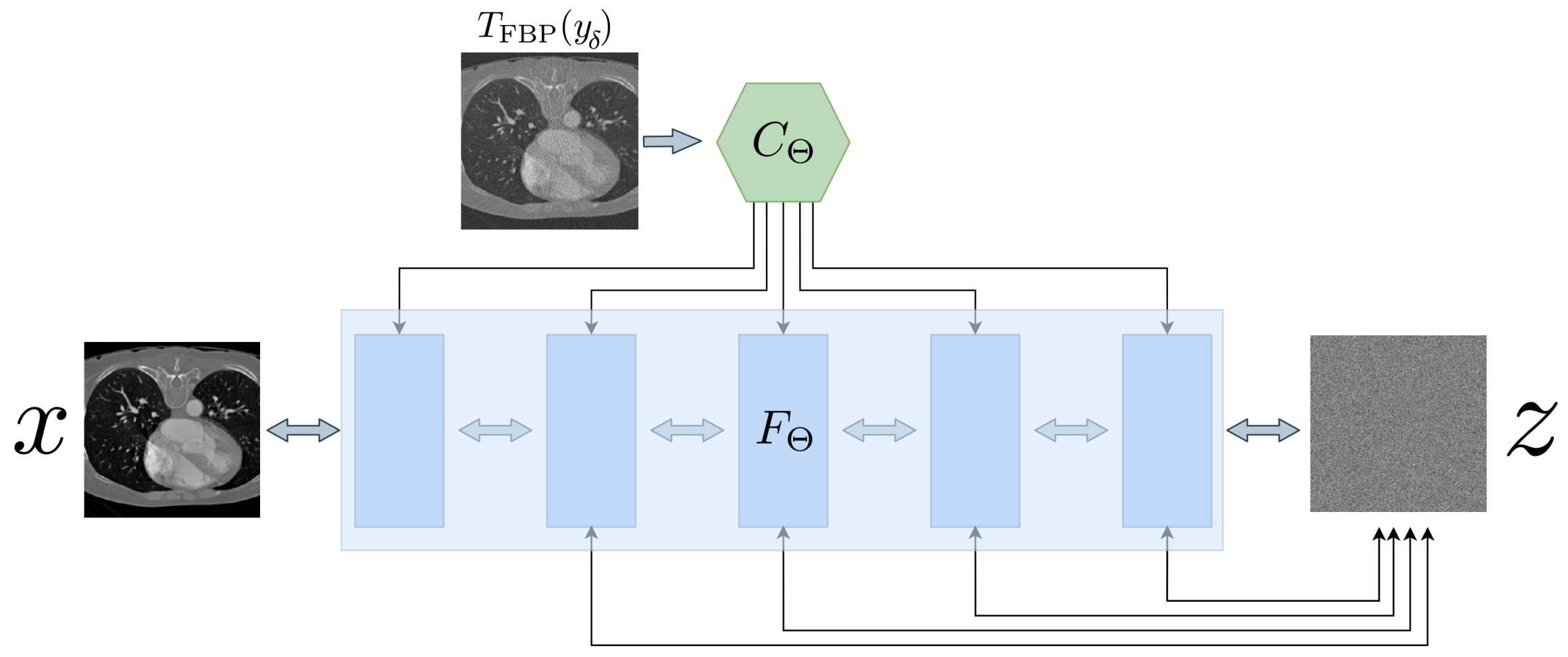
Conditional invertible neural networks (CINN) are a relatively new approach for solving inverse problems [47,80]. Models of this type consist of two network parts (cf. Figure A4). An invertible network F represents a learned transformation between the (unknown) distribution X of the ground truth data and a standard probability distribution Z , e.g., a Gaussian distribution. The second building block is a conditioning network C, which includes physical knowledge about the problem and encodes information from the measured data as an additional input to F.
A CINN was successfully applied to the task of low-dose CT reconstruction by Denker et al. [48]. Their model uses a multi-scale convolutional architecture as proposed in [81] and is built upon the FrEIA (https://github.com/VLL-HD/FrEIA, last accessed: 1 March 2021) python library. For the experiments in this paper, several improvements over the design in [48] are incorporated. The structure of the invertible network F and the conditioning network C are simplified. Using additive coupling layers [82] with Activation Normalization [83] improves stability of the training. Replacing downsampling operations with a learned version from Etmann et al. [63] prevents checkerboard artifacts and enhances the overall reconstruction quality. In addition, the negative log-likelihood (NLL) loss is combined with a weighted mean-squared error (MSE) term
min Θ [ log p Z ( F Θ ( x , C Θ y δ ) ) + log | det ( J F Θ x , C Θ y δ ) | + α MSE ( F Θ 1 z , C Θ y δ , x ) ] .
The applied network has 5 different downsampling scales, where both spatial dimensions are reduced by factor 2. Simultaneously, the number of channels increases by a factor of 4, making the operation invertible. After each downsampling step, half the channels are split of and send directly to the output layer. In total, the network has around 6.5 million parameters. It is trained with the Adam optimizer and a learning rate of 0.0005 for at most 200 epochs using batch size 4 (per GPU) on LoDoPaB-CT and for at most 32 epochs using batch size 3 on the apple data. The best model according to the validation loss is selected. A Gaussian distribution is chosen for Z . The MSE weight is set to α = 1.0 . After training, the reconstructions are generated as a conditioned mean over K = 1000 sample reconstructions from the Gaussian distribution (cf. Algorithm A2).
Figure A4. Architecture of the conditional invertible neural network. The ground truth image x is transformed by F Θ to a Gaussian distributed z. Adapted from [48].
Jimaging 07 00044 g0a4
Algorithm A2 Conditional Invertible Neural Network (CINN).
Given a noisy measurement, y δ , an invertible neural network F and a conditioning network C. Let K N be the number of random samples that should be drawn from a normal distribution N 0 , I . The algorithm calculates the mean and variance of the conditioned reconstructions.
1.
   Calculate FBP: c 0 = T FBP y δ .
2.
   Calculate outputs of the conditioning: c = C Θ c 0
3.
   for   k = 1 : K
4.
     z [ k ] N 0 , I
5.
     x ^ [ k ] = F 1 ( z [ k ] , c )
6.
   end
7.
   Calculate mean: x ^ = 1 K k x ^ [ k ]
8.
   Calculate variance: σ ^ = 1 K k x ^ [ k ] x ^ 2

Appendix A.6. ISTA U-Net

The ISTA U-Net [42] is a relatively new approach based on the encoder-decoder structure of the original U-Net. The authors draw parallels from the supervised training of U-Nets to task-driven dictionary learning and sparse coding. For the ISTA U-Net the encoder is replaced by a sparse representation of the input vector and the decoder is linearized by removing all non-linearities, batch normalization and additive biases (cf. Figure A5). Given a data set of measurements and ground truth pairs { y δ i , x i } i = 1 M the training problem can be formulated as a bi-level optimization problem
min { θ , γ } , λ > 0 1 M i = 1 M 1 2 D γ α y δ i , θ x i 2 2 where α y δ i , θ =   arg min α 0 1 2 D θ α y δ i 2 2 + λ α 1 ,
where ⊙ denotes the Hadamard product. Using an encoder dictionary D θ the corresponding sparse code α θ can be determined with the iterative thresholding algorithm (ISTA, [84]) with an additional non-negativity constraint for the sparse code. Liu et al. [42] use a learned variant of ISTA, called LISTA [85], to compute the sparse code. LISTA works by unrolling ISTA for a fixed number of K iterations
α y δ , θ [ k ] = ReLU α y δ , θ [ k 1 ] + η D κ T y δ D θ α y δ , θ [ k 1 ] η λ ,
with k = 1 , , K . In their framework they additionally untie the parameters for D κ and D θ , although both dictionaries have the same structure. The forward pass of the network is given in Algorithm A3.
For all experiments, K = 5 unrolled ISTA iterations were used. On LoDoPaB-CT, five scales with hidden layer widths 1024, 512, 256, 128, 64 were used and the lasso parameters λ were initialized with 10 3 . For the Apple CT datasets, the network appeared to be relatively sensitive with respect to the hyperparameter choices. For the noise-free data (Dataset A), five scales with hidden layer widths 512, 256, 128, 64, 32 were used and λ was initialized with 10 5 . For Datasets B and C, six scales, but less wide hidden layers, namely 512, 256, 128, 64, 32, 16, were used and λ was initialized with 10 4 . In all experiments, input FBPs computed with Hann filtering and no frequency scaling were used. A ReLU activation was applied to the network output. The network was trained by minimizing the mean squared error loss using the Adam optimizer. For LoDoPaB-CT, the network was trained for 20 epochs with a learning rate starting from 2 × 10 4 , reduced by cosine annealing to 1 × 10 5 , using batch size 2. For the Apple CT datasets, the network was trained for at most 80 epochs with a learning rate starting from 1 × 10 4 , reduced by cosine annealing to 1 × 10 5 , using batch size 1, whereby the model with the highest PSNR on the validation set was selected.
Source code is publicly available in a github repository (https://github.com/liutianlin0121/ISTA-U-Net, last accessed: 1 March 2021). A slightly modified copy of the code used for training on the Apple CT datasets is also contained in our github repository (https://github.com/jleuschn/learned_ct_reco_comparison_paper, last accessed: 1 March 2021).
Figure A5. Architecture of the ISTA U-Net adapted from [42]. The sparse code α replaces the downsampling part in the standard U-Net (cf. Figure A2).
Jimaging 07 00044 g0a5
Algorithm A3 ISTA U-Net.
Given a noisy input y δ , learned dictionaries D κ , D θ , D γ and learned step sizes η and λ the reconstruction using the ISTA U-Net can be computed as follows.
1.
   Calculate FBP: x ^ = T FBP ( y δ )
2.
   Initialize α y δ [ 0 ] = 0
3.
   for   k = 1 : K
4.
     α y δ [ k ] = ReLU α y δ [ k 1 ] + η D κ T x ^ D θ α y δ [ i 1 ] η λ
5.
   end
6.
   return x ^ = D γ α y δ [ K ]

Appendix A.7. Deep Image Prior with TV Denoising

The deep image prior (DIP) [86] takes a special role among the listed neural network approaches. In general, a DIP network F is not previously trained and, therefore, omits the problem of ground truth acquisition. Instead, the parameters Θ are adjusted iteratively during the reconstruction process by gradient descent steps (cf. Algorithm A4). The main objective is to minimize the data discrepancy of the output of the network for a fixed random input z
min Θ D Y A F Θ ( z ) , y δ .
The number of iterations have a great influence on the reconstruction quality: While too few can result in an overall bad image, too many can cause overfitting to the noise of the measurement. The general regularization strategy for this problem is a combination of early stopping and the architecture itself [87], where the prior is related to the implicit structural bias of the network. Especially convolutional networks, in combination with gradient descent, fit natural images faster than noise and learn to construct them from low to high frequencies [86,88,89].
The loss function (A1) can also be combined with classical regularization. Baguer et al. [34] add a weighted anisotropic total variation (TV) term and apply their approach to low-dose CT measurements. The method DIP + TV is also used for this comparison. The network architecture is based on the same U-Net as for the FBP U-Net post-processing (cf. Appendix A.2). It has 6 different scales with 128 channels each and a skip-channel setup of ( 0 , 0 , 0 , 0 , 4 , 4 ) . The data discrepancy D Y was measured with a Poisson loss (see Equation (9)) and the weight for TV was chosen as α = 7.0 . Gradient descent was performed for K = 17 , 000 iterations with a stepsize of 5 × 10 4 .
Algorithm A4 Deep Image Prior + Total Variation (DIP + TV).
Given a noisy measurement y δ , a neural network F Θ with initial parameterization Θ [ 0 ] , forward operator A and a fixed random input z. The reconstruction x ^ is calculated iteratively over a number of K N iterations:
1.
   for   k = 1 : K
2.
    Evaluate loss: L = D A F Θ [ k 1 ] ( z ) , y δ + α TV F Θ [ k 1 ] ( z )
3.
    Calculate gradients: Θ [ k 1 ] = Θ L
4.
    Update parameters: Θ [ k ] = Optimizer Θ [ k 1 ] , Θ [ k 1 ]
5.
    Current reconstruction: x ^ [ k ] = F Θ [ k ] ( z )
6.
   end

Appendix A.8. iCTU-Net

The iCTU-Net is based on the iCT-Net by Li et al. [29], which in turn is inspired by the common filtered back-projection. The reconstruction process is learned end-to-end, that is, the sinogram is the input of the network and the output is the reconstructed image. The full network architecture is shown in Figure A6.
First, disturbances in the raw measurement data, such as excessive noise, are suppressed as much as possible via 3 × 3 convolutions (refining layers). The corrected sinogram is then filtered using 10 × 1 convolutions (filtering layers). The filtered sinogram maintains the size of the input sinogram. Afterwards, the sinogram is back-projected into the image space. This is realized by a d × 1 convolution with N 2 output channels without padding, where d is the number of detectors in the sinogram and N is the output image size. This convolution corresponds to a fully connected layer for each viewing angle, as it connects every detector element with every pixel in the image space. The results for each view are reshaped to N × N sized images and rotated according to the acquisition angle. A 1 × 1 convolution combines all views into the back projected image. Finally, a U-Net further refines the image output.
To significantly lower the GPU memory requirements, an initial convolutional layer with stride 1 × 2 was added, to downsample the LoDoPaB sinograms from 1000 to 500 projection angles. For the apple reconstruction the number of detector elements d and the output image size N were halved. After reconstruction the image size was doubled again using linear interpolation. Training was performed using the Adam optimizer with a learning rate of 0.001 and batch size 1. For LoDoPaB-CT the mean squared error loss and for Apple CT the SSIM loss function was used. The network was trained for 2 epochs on LoDoPaB-CT and for at most 60 epochs on the Apple CT datasets, without validation based model selection (i.e., no automated early stopping).
Figure A6. Architecture of the iCTU-Net.
Jimaging 07 00044 g0a6

Appendix B. Classical Reconstruction Methods

Appendix B.1. Filtered Back-Projection (FBP)

The Radon transform [10] maps (or projects) a function x ( u ) , u = ( u 1 , u 2 ) , defined on a two-dimensional plane to a function A x ( s , φ ) defined on a two-dimensional space of lines, which are parameterized by distance to the origin, s and the angle φ of the normal. The Radon transform is given by
A x ( s , φ ) : = R x s cos ( φ ) sin ( φ ) +   t sin ( φ ) cos ( φ ) d t ,
A simple inversion idea consists in back-projecting the intensities A x ( s , φ ) to those positions u in the image x ( u ) that lie on the corresponding lines parameterized by s and φ , that is, those positions that contribute to the respective measured intensity. Mathematically, the back-projection is described by the adjoint Radon transform A * , also provided in [10]. To obtain an inversion formula, the projections A x need to be filtered before the back-projection (see e.g., [36] for a derivation and an alternative formula applying a filter after obtaining the back-projection A * A x ). A generic FBP reconstruction formula reads
x ^ = 1 2 A * F 1 | · | W F y δ ,
where F denotes the one-dimensional Fourier transform along the detector pixel dimension s, | · | denotes the Ram-Lak filter, which multiplies each frequency component with the absolute value of the frequency, and W is a low-pass filter (applying a window function). While from perfect projections A x ( s , φ ) exact recovery of x ( u ) is possible by choosing a rectangular window function for W, in practice W is also used to reduce high frequency components. This stabilizes the inversion by reducing the impact of noise present in higher frequencies. Typical choices for W are the Hann or the Cosine window. Sometimes the resulting weighting function is additionally shrunk along the frequency axis with a frequency scaling factor, which leads to removal of all frequency components above a threshold frequency.
For all experiments the implementation of ODL [90] was used in conjunction with the ASTRA toolbox [91]. Suitable hyperparameters have been determined based on the performance on validation samples and are listed in Table A1. The FBPs used for post-processing networks were computed with the Hann window and without frequency scaling. The Hann window thereby serves as a pre-processing step for the network and the frequency scaling was omitted in order to keep all information available.
Table A1. Hyperparameters for filtered back-projection (FBP).
WindowFrequency Scaling
LoDoPaB-CT Dataset Hann0.641
Apple CT Dataset A
(Noise-free)
50 anglesCosine0.11
10 anglesCosine0.013
5 anglesHann0.011
2 anglesHann0.011
Apple CT Dataset B
(Gaussian noise)
50 anglesCosine0.08
10 anglesCosine0.013
5 anglesHann0.011
2 anglesHann0.011
Apple CT Dataset C
(Scattering)
50 anglesCosine0.09
10 anglesHann0.018
5 anglesHann0.011
2 anglesHann0.009

Appendix B.2. Conjugate Gradient Least Squares

The Conjugate Gradient Least Squares (CGLS) method is the modification of the well-known Conjugate Gradient [52] where the CG method is applied to solve the least squares problem A T A x ^ = A T y δ . Here, A R m × n is the geometry matrix, y δ R m × 1 is the measured data and x ^ R n × 1 is the reconstruction. CGLS is a popular method in signal and image processing for its simple and computationally inexpensive implementation and fast convergence. The method is given in Algorithm A5, codes from [92].
Our implementation also includes a non-negativity step (negative pixel values equal to zero), applied to the final iterated solution. There is no parameter-tuning done for this implementation since the only user-defined parameter is the maximum number of iterations, K.
Algorithm A5 Conjugate Gradient Least Squares (CGLS).
Given a geometry matrix, A, a data vector y and a zero solution vector x ^ [ 0 ] = 0 (a black image) as the starting point, the algorithm below gives the solution at kth iteration.
1.
   Initialise the direction vector as d [ 0 ] = A T y δ .
2.
   for   k = 1 : K
3.
     q [ k 1 ] = A d [ k 1 ] , α = d [ k 1 ] 2 2 / q [ k 1 ] 2 2
4.
    Update: x ^ [ k ] = x ^ [ k 1 ] + α d [ k 1 ] , b [ k ] = b [ k 1 ] α q [ k 1 ]
5.
    Reinitialise: q [ k ] = A T q [ k 1 ] , β = q [ k ] 2 2 / d [ k 1 ] 2 2 , d [ k ] = q [ k ] + β d [ k 1 ]
6.
   end

Appendix B.3. Total Variation Regularization

Regularizing the reconstruction process with anisotropic total variation (TV) is a common approach for CT [93]. In addition to the data discrepancy D , a weighted regularization term is added to the minimization problem
T TV y δ arg min x D A x , y δ + α h x 1 + v x 1 ,
where h and v denote gradients in horizontal and vertical image direction, respectively, and can be approximated by finite differences in the discrete setting. TV penalizes variations in the image, e.g., from noise. Therefore, it is often applied in a denoising role. A number of optimization algorithms exist for minimizing (A2) [54]. The choice and exact formulation depend on the properties of the data discrepancy term.
For our comparison, we use the standard DIV α implementation of TV. Adam gradient descent minimizes (A2), whereby the gradients are calculated by automatic differentiation in PyTorch [94] (cf. Algorithm A6).
For the data discrepancy D , a Poisson loss (see (9)) was used for LoDoPaB-CT, while the MSE was used for the Apple CT datasets. Suitable hyperparameters have been determined based on the performance on validation samples and are listed in Table A2. For lower numbers of angles, a very high number of iterations was found to be beneficial, leading to very slow reconstruction (≈17 min per image for K = 150,000 iterations, which we chose to be the maximum). In all cases an FBP with Hann window and frequency scaling factor 0.1 was used as initial reconstruction.
Table A2. Hyperparameters for total variation regularization (TV).
DiscrepancyIterationsStep Size α
LoDoPaB-CT Dataset Pois 50000.00120.56
Apple CT Dataset A
(Noise-free)
50 anglesMSE600 3 × 10 2 2 × 10 12
10 anglesMSE75,000 3 × 10 3 6 × 10 12
5 anglesMSE146,000 1.5 × 10 3 1 × 10 11
2 anglesMSE150,000 1 × 10 3 2 × 10 11
Apple CT Dataset B
(Gaussian noise)
50 anglesMSE900 3 × 10 4 2 × 10 10
10 anglesMSE66,000 2 × 10 5 6 × 10 10
5 anglesMSE100,000 1 × 10 5 3 × 10 9
2 anglesMSE149,000 1 × 10 5 4 × 10 9
Apple CT Dataset C
(Scattering)
50 anglesMSE400 5 × 10 3 1 × 10 11
10 anglesMSE13,000 2 × 10 3 4 × 10 11
5 anglesMSE149,000 1 × 10 3 4 × 10 11
2 anglesMSE150,000 4 × 10 4 6 × 10 11
Algorithm A6 Total Variation Regularization (TV).
Given a noisy measurement y δ , an initial reconstruction x ^ [ 0 ] , a weight α > 0 and a maximum number of iterations K.
1.
   for   k = 1 : K
2.
    Evaluate loss: L = D A x ^ [ k 1 ] , y δ + α h x ^ [ k 1 ] 1 + v x ^ [ k 1 ] 1
3.
    Calculate gradients: x ^ [ k 1 ] = x L
4.
    Update: x ^ [ k ] = Optimizer x ^ [ k 1 ] , x ^ [ k 1 ]
5.
   end

Appendix C. Further Results

Table A3. Standard deviation of PSNR and SSIM (adapted to the data range of each ground truth image) for the different noise settings on the 100 selected Apple CT test images.
Noise-FreeStandard Deviation of PSNRStandard Deviation of SSIM
Number of Angles501052501052
Learned Primal-Dual1.511.631.972.580.0220.0160.0140.022
ISTA U-Net1.401.772.122.130.0180.0180.0220.037
U-Net1.561.612.281.630.0210.0190.0250.031
MS-D-CNN1.511.651.812.090.0210.0200.0240.022
CINN1.401.641.992.170.0160.0190.0230.027
iCTU-Net1.682.451.921.930.0240.0270.0300.028
TV1.601.291.211.490.0220.0410.0290.023
CGLS0.690.482.940.700.0140.0270.0290.039
FBP0.800.580.540.500.0210.0230.0280.067
Gaussian NoiseStandard Deviation of PSNRStandard Deviation of SSIM
Number of Angles501052501052
Learned Primal-Dual1.561.632.002.790.0210.0180.0210.022
ISTA U-Net1.701.762.272.120.0250.0210.0220.038
U-Net1.661.591.992.220.0230.0200.0250.026
MS-D-CNN1.661.751.791.790.0250.0240.0190.022
CINN1.531.511.622.060.0230.0170.0170.020
iCTU-Net1.982.061.891.910.0310.0320.0390.027
TV1.381.261.091.620.0360.0470.0390.030
CGLS0.780.491.760.680.0140.0260.0290.037
FBP0.910.580.540.500.0280.0230.0280.067
Scattering NoiseStandard Deviation of PSNRStandard Deviation of SSIM
Number of Angles501052501052
Learned Primal-Dual1.911.801.712.470.0170.0160.0160.060
ISTA U-Net1.481.592.051.810.0230.0190.0190.038
U-Net1.761.561.811.470.0150.0210.0270.024
MS-D-CNN2.041.781.852.030.0230.0220.0150.020
CINN1.821.922.322.250.0190.0240.0290.030
iCTU-Net1.912.091.782.290.0300.0310.0330.040
TV2.532.441.861.590.0670.0760.0350.062
CGLS2.381.321.710.950.0200.0200.0260.032
FBP2.230.970.800.680.0440.0250.0230.058
Table A4. PSNR-FR and SSIM-FR (computed with fixed data range 0.0129353 for all images) for the different noise settings on the 100 selected Apple CT test images. Best results are highlighted in gray.
Noise-FreePSNR-FRSSIM-FR
Number of Angles501052501052
Learned Primal-Dual45.3342.4737.4128.610.9710.9570.9350.872
ISTA U-Net45.4841.1534.9327.100.9670.9440.9070.823
U-Net46.2440.1334.3826.390.9750.9170.9110.830
MS-D-CNN46.4741.0035.0627.170.9750.9360.8980.808
CINN46.2041.4634.4326.070.9750.9580.8960.838
iCTU-Net42.6936.5732.2425.900.9570.9380.9200.861
TV45.8935.6128.6622.570.9760.9040.7460.786
CGLS39.6628.4319.2221.870.9010.7440.6540.733
FBP37.0123.7122.1220.580.8560.7110.5960.538
Gaussian NoisePSNR-FRSSIM-FR
Number of Angles501052501052
Learned Primal-Dual43.2440.3836.5428.030.9610.9440.9270.823
ISTA U-Net42.6540.1735.0927.320.9560.9420.9160.826
U-Net43.0939.4534.4226.470.9610.9240.9040.843
MS-D-CNN43.2839.8234.6026.500.9620.9320.8860.797
CINN43.3938.5033.1926.600.9660.9040.8780.816
iCTU-Net39.5136.3831.2926.060.9390.9320.9050.867
TV38.9833.7328.4522.700.9390.8830.7700.772
CGLS33.9827.7121.5221.730.8840.7480.6680.734
FBP34.5023.7022.1220.580.8390.7110.5960.538
Scattering NoisePSNR-FRSSIM-FR
Number of Angles501052501052
Learned Primal-Dual44.4240.8033.6927.600.9670.9540.9120.760
ISTA U-Net42.5538.9534.0326.570.9590.9220.8870.816
U-Net41.5839.5233.5525.560.9320.9100.8770.828
MS-D-CNN44.6640.1334.3426.810.9690.9270.8890.796
CINN45.1840.6934.6625.760.9760.9520.9360.878
iCTU-Net32.8829.4627.8624.930.9310.9010.8960.873
TV27.7126.7624.4821.150.9030.7990.6740.743
CGLS27.4624.8920.6420.800.8960.7380.6590.736
FBP27.6322.4220.8819.680.8780.7010.5890.529
Table A5. Standard deviation of PSNR-FR and SSIM-FR (computed with fixed data range 0.0129353 for all images) for the different noise settings on the 100 selected Apple CT test images.
Noise-FreeStandard Deviation of PSNR-FRStandard Deviation of SSIM-FR
Number of Angles501052501052
Learned Primal-Dual1.491.672.032.540.0070.0060.0100.019
ISTA U-Net1.371.822.212.210.0050.0100.0200.034
U-Net1.531.662.331.680.0060.0120.0190.026
MS-D-CNN1.461.711.902.150.0060.0110.0210.015
CINN1.351.652.092.210.0040.0070.0230.025
iCTU-Net1.822.542.031.910.0140.0170.0200.023
TV1.541.321.281.360.0060.0230.0260.018
CGLS0.710.512.960.560.0090.0290.0330.045
FBP0.770.460.380.410.0110.0150.0290.088
Gaussian NoiseStandard Deviation of PSNR-FRStandard Deviation of SSIM-FR
Number of Angles501052501052
Learned Primal-Dual1.521.682.042.830.0060.0080.0130.016
ISTA U-Net1.651.782.362.170.0080.0100.0180.034
U-Net1.611.622.052.240.0070.0120.0190.024
MS-D-CNN1.621.801.841.840.0080.0110.0150.014
CINN1.501.591.652.090.0070.0160.0170.019
iCTU-Net2.072.121.931.900.0200.0210.0260.024
TV1.301.261.151.500.0140.0270.0300.019
CGLS0.630.451.760.530.0120.0280.0340.043
FBP0.830.460.380.410.0140.0150.0290.088
Scattering NoiseStandard Deviation of PSNR-FRStandard Deviation of SSIM-FR
Number of Angles501052501052
Learned Primal-Dual1.921.851.812.510.0050.0070.0140.038
ISTA U-Net1.561.682.171.890.0100.0140.0140.035
U-Net1.721.631.911.590.0100.0120.0240.024
MS-D-CNN2.021.841.962.080.0080.0120.0160.019
CINN1.741.972.412.210.0050.0110.0160.022
iCTU-Net1.962.141.792.320.0160.0230.0220.030
TV2.432.351.801.490.0480.0740.0400.051
CGLS2.281.241.670.830.0160.0210.0300.035
FBP2.140.870.660.550.0280.0160.0200.078
Figure A7. PSNR and SSIM depending on the number of angles on the Apple CT datasets.
Jimaging 07 00044 g0a7
Figure A8. PSNR and SSIM compared for all noise settings and numbers of angles.
Jimaging 07 00044 g0a8
Table A6. Mean and standard deviation of the mean squared difference between the noisy measurements and the forward-projected reconstructions, respectively the noise-free measurements, on the 100 selected Apple CT test images.
Noise FreeMSE × 10 9
Number of Angles501052
Learned Primal-Dual 0.083 ± 0.027 0.405 ± 0.156 1.559 ± 0.543 2.044 ± 1.177
ISTA U-Net 0.323 ± 0.240 0.633 ± 0.339 2.672 ± 1.636 17.840 ± 12.125
U-Net 0.097 ± 0.093 1.518 ± 0.707 5.011 ± 3.218 31.885 ± 17.219
MS-D-CNN 0.117 ± 0.088 0.996 ± 0.595 3.874 ± 2.567 20.879 ± 12.038
CINN 0.237 ± 0.259 1.759 ± 0.348 3.798 ± 2.176 33.676 ± 16.747
iCTU-Net 2.599 ± 3.505 6.686 ± 8.469 14.508 ± 16.694 18.876 ± 12.553
TV 0.002 ± 0.000 0.001 ± 0.000 0.000 ± 0.000 0.001 ± 0.000
CGLS 1.449 ± 0.299 29.921 ± 6.173 752.997 ± 722.151 22.507 ± 13.748
FBP 12.229 ± 3.723 89.958 ± 9.295 159.746 ± 15.596 273.054 ± 114.552
Ground truth 0.000 ± 0.000 0.000 ± 0.000 0.000 ± 0.000 0.000 ± 0.000
Gaussian NoiseMSE × 10 9
Number of Angles501052
Learned Primal-Dual 19.488 ± 5.923 19.813 ± 5.851 20.582 ± 5.690 32.518 ± 4.286
ISTA U-Net 19.438 ± 5.943 20.178 ± 6.060 21.167 ± 6.052 32.435 ± 9.782
U-Net 19.802 ± 6.247 22.114 ± 6.364 23.645 ± 6.527 38.895 ± 17.211
MS-D-CNN 19.348 ± 5.921 20.056 ± 5.930 23.080 ± 5.959 47.625 ± 18.133
CINN 19.429 ± 5.891 21.069 ± 5.663 29.517 ± 7.296 42.876 ± 15.471
iCTU-Net 25.645 ± 9.602 25.421 ± 9.976 38.179 ± 22.887 41.956 ± 15.942
TV 18.760 ± 5.674 18.107 ± 5.395 20.837 ± 5.510 18.514 ± 5.688
CGLS 87.892 ± 23.312 71.526 ± 17.600 262.616 ± 151.655 98.520 ± 18.245
FBP 31.803 ± 9.558 109.430 ± 14.107 179.260 ± 19.744 292.692 ± 109.223
Ground truth 19.538 ± 6.029 19.505 ± 6.019 19.551 ± 6.028 19.483 ± 6.086
Scattering NoiseMSE × 10 9
Number of Angles501052
Learned Primal-Dual 541.30 ± 311.82 579.14 ± 317.59 549.30 ± 328.41 435.07 ± 260.02
ISTA U-Net 553.64 ± 355.14 557.03 ± 342.67 575.94 ± 338.82 522.33 ± 365.58
U-Net 629.62 ± 353.54 635.91 ± 343.31 550.54 ± 340.27 642.20 ± 295.46
MS-D-CNN 579.86 ± 332.39 585.18 ± 331.93 533.35 ± 331.21 606.55 ± 365.25
CINN 638.80 ± 355.24 619.47 ± 353.47 603.53 ± 362.96 649.30 ± 409.83
iCTU-Net 622.51 ± 348.32 622.63 ± 335.28 652.18 ± 359.00 573.46 ± 324.00
TV 3.35 ± 5.02 3.19 ± 4.83 2.96 ± 4.47 2.55 ± 6.33
CGLS 6.40 ± 6.39 34.71 ± 8.16 286.20 ± 205.42 19.92 ± 14.01
FBP 12.48 ± 6.88 73.53 ± 10.19 144.70 ± 15.82 221.79 ± 59.71
Ground truth 610.47 ± 355.25 610.40 ± 355.16 611.23 ± 354.51 620.11 ± 386.79
Figure A9. Example of an artifact produced by DIP + TV, which has only minor impact on the evaluated metrics (especially the SSIM). The area containing the artifact is marked with a red circle.
Jimaging 07 00044 g0a9

Appendix D. Training Curves

Figure A10. Training curves of Learned Primal-Dual on the Apple CT dataset. Dashed lines: average validation loss computed after every full training epoch; solid lines: running average of training loss since start of epoch. Duration of 20 epochs on full dataset: ≈10–17 days, varying with the number of angles.
Jimaging 07 00044 g0a10
Figure A11. Training curves of ISTA U-Net on the Apple CT dataset. Dashed lines: average validation PSNR in decibel computed after every full training epoch; marks: selected model. Duration of 20 epochs on full dataset: ≈10 days for hidden layer width 32+ and 5 scales, respectively ≈5.5 days for hidden layer width 16+ and 6 scales.
Jimaging 07 00044 g0a11
Figure A12. Training curves of U-Net on the Apple CT dataset. Dashed lines: average validation loss computed after every full training epoch; solid lines: running average of training loss since start of epoch. Duration of 20 epochs on full dataset: ≈1.5 days.
Jimaging 07 00044 g0a12
Figure A13. Training curves of MS-D-CNN on the Apple CT dataset. Dashed lines: average validation loss computed after every full training epoch; solid lines: running average of training loss since start of epoch. Duration of 20 epochs on full dataset: ≈20 days.
Jimaging 07 00044 g0a13
Figure A14. Training curves of CINN on the Apple CT dataset. Dashed lines: average validation loss computed after every full training epoch; solid lines: running average of training loss (at every 50-th step) since start of epoch. For some of the trainings, the epochs were divided into multiple shorter ones. Duration of 20 epochs on full dataset: ≈2.5 days (using 2 GPUs).
Jimaging 07 00044 g0a14
Figure A15. Training curves of iCTU-Net on the Apple CT dataset. Opaque lines: loss for a validation sample (after every 500-th step); semi-transparent lines: training loss (at every 500-th step). Duration of 20 epochs on full dataset: ≈3 days.
Jimaging 07 00044 g0a15

References

  1. Liguori, C.; Frauenfelder, G.; Massaroni, C.; Saccomandi, P.; Giurazza, F.; Pitocco, F.; Marano, R.; Schena, E. Emerging clinical applications of computed tomography. Med. Devices 2015, 8, 265. [Google Scholar]
  2. National Lung Screening Trial Research Team. Reduced lung-cancer mortality with low-dose computed tomographic screening. N. Engl. J. Med. 2011, 365, 395–409. [Google Scholar] [CrossRef] [Green Version]
  3. Yoo, S.; Yin, F.F. Dosimetric feasibility of cone-beam CT-based treatment planning compared to CT-based treatment planning. Int. J. Radiat. Oncol. Biol. Phys. 2006, 66, 1553–1561. [Google Scholar] [CrossRef]
  4. Swennen, G.R.; Mollemans, W.; Schutyser, F. Three-dimensional treatment planning of orthognathic surgery in the era of virtual imaging. J. Oral Maxillofac. Surg. 2009, 67, 2080–2092. [Google Scholar] [CrossRef]
  5. De Chiffre, L.; Carmignato, S.; Kruth, J.P.; Schmitt, R.; Weckenmann, A. Industrial applications of computed tomography. CIRP Ann. 2014, 63, 655–677. [Google Scholar] [CrossRef]
  6. Mees, F.; Swennen, R.; Van Geet, M.; Jacobs, P. Applications of X-ray Computed Tomography in the Geosciences; Special Publications; Geological Society: London, UK, 2003; Volume 215, pp. 1–6. [Google Scholar]
  7. Morigi, M.; Casali, F.; Bettuzzi, M.; Brancaccio, R.; d’Errico, V. Application of X-ray computed tomography to cultural heritage diagnostics. Appl. Phys. A 2010, 100, 653–661. [Google Scholar] [CrossRef]
  8. Coban, S.B.; Lucka, F.; Palenstijn, W.J.; Van Loo, D.; Batenburg, K.J. Explorative Imaging and Its Implementation at the FleX-ray Laboratory. J. Imaging 2020, 6, 18. [Google Scholar] [CrossRef] [Green Version]
  9. McCollough, C.H.; Bartley, A.C.; Carter, R.E.; Chen, B.; Drees, T.A.; Edwards, P.; Holmes, D.R., III.; Huang, A.E.; Khan, F.; Leng, S.; et al. Low-dose CT for the detection and classification of metastatic liver lesions: Results of the 2016 Low Dose CT Grand Challenge. Med Phys. 2017, 44, e339–e352. [Google Scholar] [CrossRef] [PubMed] [Green Version]
  10. Radon, J. On the determination of functions from their integral values along certain manifolds. IEEE Trans. Med Imaging 1986, 5, 170–176. [Google Scholar] [CrossRef]
  11. Natterer, F. The mathematics of computerized tomography (classics in applied mathematics, vol. 32). Inverse Probl. 2001, 18, 283–284. [Google Scholar]
  12. Boas, F.E.; Fleischmann, D. CT artifacts: Causes and reduction techniques. Imaging Med. 2012, 4, 229–240. [Google Scholar] [CrossRef] [Green Version]
  13. Wang, G.; Ye, J.C.; Mueller, K.; Fessler, J.A. Image Reconstruction is a New Frontier of Machine Learning. IEEE Trans. Med. Imaging 2018, 37, 1289–1296. [Google Scholar] [CrossRef] [PubMed]
  14. Sidky, E.Y.; Pan, X. Image reconstruction in circular cone-beam computed tomography by constrained, total-variation minimization. Phys. Med. Biol. 2008, 53, 4777. [Google Scholar] [CrossRef] [Green Version]
  15. Niu, S.; Gao, Y.; Bian, Z.; Huang, J.; Chen, W.; Yu, G.; Liang, Z.; Ma, J. Sparse-view X-ray CT reconstruction via total generalized variation regularization. Phys. Med. Biol. 2014, 59, 2997. [Google Scholar] [CrossRef] [PubMed]
  16. Hestenes, M.R.; Stiefel, E. Methods of conjugate gradients for solving linear systems. J. Res. Natl. Bur. Stand. 1952, 49, 409–436. [Google Scholar] [CrossRef]
  17. Arridge, S.; Maass, P.; Öktem, O.; Schönlieb, C.B. Solving inverse problems using data-driven models. Acta Numer. 2019, 28, 1–174. [Google Scholar] [CrossRef] [Green Version]
  18. Lunz, S.; Öktem, O.; Schönlieb, C.B. Adversarial Regularizers in Inverse Problems. In Advances in Neural Information Processing Systems; Bengio, S., Wallach, H., Larochelle, H., Grauman, K., Cesa-Bianchi, N., Garnett, R., Eds.; Curran Associates, Inc.: Red Hook, NY, USA, 2018; Volume 31, pp. 8507–8516. [Google Scholar]
  19. Adler, J.; Öktem, O. Learned Primal-Dual Reconstruction. IEEE Trans. Med. Imaging 2018, 37, 1322–1332. [Google Scholar] [CrossRef] [Green Version]
  20. Jin, K.H.; McCann, M.T.; Froustey, E.; Unser, M. Deep Convolutional Neural Network for Inverse Problems in Imaging. IEEE Trans. Image Process. 2017, 26, 4509–4522. [Google Scholar] [CrossRef] [Green Version]
  21. Pelt, D.M.; Batenburg, K.J.; Sethian, J.A. Improving Tomographic Reconstruction from Limited Data Using Mixed-Scale Dense Convolutional Neural Networks. J. Imaging 2018, 4, 128. [Google Scholar] [CrossRef] [Green Version]
  22. Chen, H.; Zhang, Y.; Zhang, W.; Liao, P.; Li, K.; Zhou, J.; Wang, G. Low-dose CT via convolutional neural network. Biomed. Opt. Express 2017, 8, 679–694. [Google Scholar] [CrossRef]
  23. Chen, H.; Zhang, Y.; Kalra, M.K.; Lin, F.; Chen, Y.; Liao, P.; Zhou, J.; Wang, G. Low-dose CT with a residual encoder-decoder convolutional neural network. IEEE Trans. Med. Imaging 2017, 36, 2524–2535. [Google Scholar] [CrossRef]
  24. Yang, Q.; Yan, P.; Kalra, M.K.; Wang, G. CT image denoising with perceptive deep neural networks. arXiv 2017, arXiv:1702.07019. [Google Scholar]
  25. Yang, Q.; Yan, P.; Zhang, Y.; Yu, H.; Shi, Y.; Mou, X.; Kalra, M.K.; Zhang, Y.; Sun, L.; Wang, G. Low-dose CT image denoising using a generative adversarial network with Wasserstein distance and perceptual loss. IEEE Trans. Med. Imaging 2018, 37, 1348–1357. [Google Scholar] [CrossRef]
  26. Feng, R.; Rundle, D.; Wang, G. Neural-networks-based Photon-Counting Data Correction: Pulse Pileup Effect. arXiv 2018, arXiv:1804.10980. [Google Scholar]
  27. Zhu, B.; Liu, J.Z.; Cauley, S.F.; Rosen, B.R.; Rosen, M.S. Image reconstruction by domain-transform manifold learning. Nature 2018, 555, 487–492. [Google Scholar] [CrossRef] [Green Version]
  28. He, J.; Ma, J. Radon inversion via deep learning. IEEE Trans. Med. Imaging 2020, 39, 2076–2087. [Google Scholar] [CrossRef] [PubMed] [Green Version]
  29. Li, Y.; Li, K.; Zhang, C.; Montoya, J.; Chen, G.H. Learning to reconstruct computed tomography images directly from sinogram data under a variety of data acquisition conditions. IEEE Trans. Med Imaging 2019, 38, 2469–2481. [Google Scholar] [CrossRef]
  30. European Society of Radiology (ESR). The new EU General Data Protection Regulation: What the radiologist should know. Insights Imaging 2017, 8, 295–299. [Google Scholar] [CrossRef] [PubMed] [Green Version]
  31. Kaissis, G.A.; Makowski, M.R.; Rückert, D.; Braren, R.F. Secure, privacy-preserving and federated machine learning in medical imaging. Nat. Mach. Intell. 2020, 2, 305–311. [Google Scholar] [CrossRef]
  32. Leuschner, J.; Schmidt, M.; Baguer, D.O.; Maass, P. The LoDoPaB-CT Dataset: A Benchmark Dataset for Low-Dose CT Reconstruction Methods. arXiv 2020, arXiv:1910.01113. [Google Scholar]
  33. Armato, S.G., III; McLennan, G.; Bidaut, L.; McNitt-Gray, M.F.; Meyer, C.R.; Reeves, A.P.; Zhao, B.; Aberle, D.R.; Henschke, C.I.; Hoffman, E.A.; et al. The Lung Image Database Consortium (LIDC) and Image Database Resource Initiative (IDRI): A Completed Reference Database of Lung Nodules on CT Scans. Med. Phys. 2011, 38, 915–931. [Google Scholar] [CrossRef]
  34. Baguer, D.O.; Leuschner, J.; Schmidt, M. Computed tomography reconstruction using deep image prior and learned reconstruction methods. Inverse Probl. 2020, 36, 094004. [Google Scholar] [CrossRef]
  35. Armato, S.G., III; McLennan, G.; Bidaut, L.; McNitt-Gray, M.F.; Meyer, C.R.; Reeves, A.P.; Zhao, B.; Aberle, D.R.; Henschke, C.I.; Hoffman, E.A.; et al. Data From LIDC-IDRI; The Cancer Imaging Archive: Frederick, MD, USA, 2015. [Google Scholar] [CrossRef]
  36. Buzug, T. Computed Tomography: From Photon Statistics to Modern Cone-Beam CT; Springer: Berlin/Heidelberg, Germany, 2008. [Google Scholar] [CrossRef]
  37. Coban, S.B.; Andriiashen, V.; Ganguly, P.S. Apple CT Data: Simulated Parallel-Beam Tomographic Datasets; Zenodo: Geneva, Switzerland, 2020. [Google Scholar] [CrossRef]
  38. Coban, S.B.; Andriiashen, V.; Ganguly, P.S.; van Eijnatten, M.; Batenburg, K.J. Parallel-beam X-ray CT datasets of apples with internal defects and label balancing for machine learning. arXiv 2020, arXiv:2012.13346. [Google Scholar]
  39. Leuschner, J.; Schmidt, M.; Ganguly, P.S.; Andriiashen, V.; Coban, S.B.; Denker, A.; van Eijnatten, M. Source Code and Supplementary Material for “Quantitative comparison of deep learning-based image reconstruction methods for low-dose and sparse-angle CT applications”. Zenodo 2021. [Google Scholar] [CrossRef]
  40. Ronneberger, O.; Fischer, P.; Brox, T. U-net: Convolutional networks for biomedical image segmentation. In International Conference on Medical Image Computing and Computer-Assisted Intervention; Springer: Heidelberg, Germany, 2015; pp. 234–241. [Google Scholar]
  41. Zhou, Z.; Siddiquee, M.M.R.; Tajbakhsh, N.; Liang, J. Unet++: A nested u-net architecture for medical image segmentation. In Deep Learning in Medical Image Analysis and Multimodal Learning for Clinical Decision Support; Springer: Heidelberg, Germany, 2018; pp. 3–11. [Google Scholar]
  42. Liu, T.; Chaman, A.; Belius, D.; Dokmanić, I. Interpreting U-Nets via Task-Driven Multiscale Dictionary Learning. arXiv 2020, arXiv:2011.12815. [Google Scholar]
  43. Comelli, A.; Dahiya, N.; Stefano, A.; Benfante, V.; Gentile, G.; Agnese, V.; Raffa, G.M.; Pilato, M.; Yezzi, A.; Petrucci, G.; et al. Deep learning approach for the segmentation of aneurysmal ascending aorta. Biomed. Eng. Lett. 2020, 1–10. [Google Scholar]
  44. Dashti, M.; Stuart, A.M. The Bayesian Approach to Inverse Problems. In Handbook of Uncertainty Quantification; Springer International Publishing: Cham, Switzerland, 2017; pp. 311–428. [Google Scholar] [CrossRef] [Green Version]
  45. Adler, J.; Öktem, O. Deep Bayesian Inversion. arXiv 2018, arXiv:1811.05910. [Google Scholar]
  46. Goodfellow, I.; Pouget-Abadie, J.; Mirza, M.; Xu, B.; Warde-Farley, D.; Ozair, S.; Courville, A.; Bengio, Y. Generative adversarial nets. arXiv 2014, arXiv:1406.2661. [Google Scholar]
  47. Ardizzone, L.; Lüth, C.; Kruse, J.; Rother, C.; Köthe, U. Guided image generation with conditional invertible neural networks. arXiv 2019, arXiv:1907.02392. [Google Scholar]
  48. Denker, A.; Schmidt, M.; Leuschner, J.; Maass, P.; Behrmann, J. Conditional Normalizing Flows for Low-Dose Computed Tomography Image Reconstruction. arXiv 2020, arXiv:2006.06270. [Google Scholar]
  49. Hadamard, J. Lectures on Cauchy’s Problem in Linear Partial Differential Equations; Dover: New York, NY, USA, 1952. [Google Scholar]
  50. Nashed, M. A new approach to classification and regularization of ill-posed operator equations. In Inverse and Ill-Posed Problems; Engl, H.W., Groetsch, C., Eds.; Academic Press: Cambridge, MA, USA, 1987; pp. 53–75. [Google Scholar] [CrossRef]
  51. Natterer, F.; Wübbeling, F. Mathematical Methods in Image Reconstruction; Society for Industrial and Applied Mathematics: Philadelphia, PA, USA, 2001. [Google Scholar]
  52. Saad, Y. Iterative Methods for Sparse Linear Systems, 2nd ed.; Society for Industrial and Applied Mathematics: Philadelphia, PA, USA, 2003. [Google Scholar]
  53. Björck, Å.; Elfving, T.; Strakos, Z. Stability of conjugate gradient and Lanczos methods for linear least squares problems. SIAM J. Matrix Anal. Appl. 1998, 19, 720–736. [Google Scholar] [CrossRef]
  54. Chen, H.; Wang, C.; Song, Y.; Li, Z. Split Bregmanized anisotropic total variation model for image deblurring. J. Vis. Commun. Image Represent. 2015, 31, 282–293. [Google Scholar] [CrossRef]
  55. Wang, Z.; Bovik, A.C.; Sheikh, H.R.; Simoncelli, E.P. Image quality assessment: From error visibility to structural similarity. IEEE Trans. Image Process. 2004, 13, 600–612. [Google Scholar] [CrossRef] [PubMed] [Green Version]
  56. Goodfellow, I.; Bengio, Y.; Courville, A. Deep Learning; MIT Press: Cambridge, MA, USA, 2016; Available online: http://www.deeplearningbook.org (accessed on 1 March 2021).
  57. Leuschner, J.; Schmidt, M.; Ganguly, P.S.; Andriiashen, V.; Coban, S.B.; Denker, A.; van Eijnatten, M. Supplementary Material for Experiments in “Quantitative comparison of deep learning-based image reconstruction methods for low-dose and sparse-angle CT applications”. Zenodo 2021. [Google Scholar] [CrossRef]
  58. Leuschner, J.; Schmidt, M.; Baguer, D.O.; Bauer, D.; Denker, A.; Hadjifaradji, A.; Liu, T. LoDoPaB-CT Challenge Reconstructions compared in “Quantitative comparison of deep learning-based image reconstruction methods for low-dose and sparse-angle CT applications”. Zenodo 2021. [Google Scholar] [CrossRef]
  59. Leuschner, J.; Schmidt, M.; Ganguly, P.S.; Andriiashen, V.; Coban, S.B.; Denker, A.; van Eijnatten, M. Apple CT Test Reconstructions compared in “Quantitative comparison of deep learning-based image reconstruction methods for low-dose and sparse-angle CT applications”. Zenodo 2021. [Google Scholar] [CrossRef]
  60. Leuschner, J.; Schmidt, M.; Otero Baguer, D.; Erzmann, D.; Baltazar, M. DIVal Library. Zenodo 2021. [Google Scholar] [CrossRef]
  61. Knoll, F.; Murrell, T.; Sriram, A.; Yakubova, N.; Zbontar, J.; Rabbat, M.; Defazio, A.; Muckley, M.J.; Sodickson, D.K.; Zitnick, C.L.; et al. Advancing machine learning for MR image reconstruction with an open competition: Overview of the 2019 fastMRI challenge. Magn. Reson. Med. 2020, 84, 3054–3070. [Google Scholar] [CrossRef]
  62. Putzky, P.; Welling, M. Invert to Learn to Invert. In Advances in Neural Information Processing Systems; Wallach, H., Larochelle, H., Beygelzimer, A., dAlch’e-Buc, F., Fox, E., Garnett, R., Eds.; Curran Associates, Inc.: Red Hook, NY, USA, 2019; Volume 32, pp. 446–456. [Google Scholar]
  63. Etmann, C.; Ke, R.; Schönlieb, C. iUNets: Learnable Invertible Up- and Downsampling for Large-Scale Inverse Problems. In Proceedings of the 30th IEEE International Workshop on Machine Learning for Signal Processing (MLSP 2020), Espoo, Finland, 21–24 September 2020; pp. 1–6. [Google Scholar] [CrossRef]
  64. Ziabari, A.; Ye, D.H.; Srivastava, S.; Sauer, K.D.; Thibault, J.; Bouman, C.A. 2.5D Deep Learning For CT Image Reconstruction Using A Multi-GPU Implementation. In Proceedings of the 2018 52nd Asilomar Conference on Signals, Systems, and Computers, Pacific Grove, CA, USA, 28–31 October 2018; pp. 2044–2049. [Google Scholar] [CrossRef] [Green Version]
  65. Scherzer, O.; Weickert, J. Relations Between Regularization and Diffusion Filtering. J. Math. Imaging Vis. 2000, 12, 43–63. [Google Scholar] [CrossRef]
  66. Perona, P.; Malik, J. Scale-space and edge detection using anisotropic diffusion. IEEE Trans. Pattern Anal. Mach. Intell. 1990, 12, 629–639. [Google Scholar] [CrossRef] [Green Version]
  67. Mendrik, A.M.; Vonken, E.; Rutten, A.; Viergever, M.A.; van Ginneken, B. Noise Reduction in Computed Tomography Scans Using 3-D Anisotropic Hybrid Diffusion With Continuous Switch. IEEE Trans. Med Imaging 2009, 28, 1585–1594. [Google Scholar] [CrossRef] [PubMed]
  68. Adler, J.; Lunz, S.; Verdier, O.; Schönlieb, C.B.; Öktem, O. Task adapted reconstruction for inverse problems. arXiv 2018, arXiv:1809.00948. [Google Scholar]
  69. Boink, Y.E.; Manohar, S.; Brune, C. A partially-learned algorithm for joint photo-acoustic reconstruction and segmentation. IEEE Trans. Med. Imaging 2019, 39, 129–139. [Google Scholar] [CrossRef]
  70. Handels, H.; Deserno, T.M.; Maier, A.; Maier-Hein, K.H.; Palm, C.; Tolxdorff, T. Bildverarbeitung für die Medizin 2019; Springer Fachmedien Wiesbaden: Wiesbaden, Germany, 2019. [Google Scholar] [CrossRef]
  71. Mason, A.; Rioux, J.; Clarke, S.E.; Costa, A.; Schmidt, M.; Keough, V.; Huynh, T.; Beyea, S. Comparison of objective image quality metrics to expert radiologists’ scoring of diagnostic quality of MR images. IEEE Trans. Med. Imaging 2019, 39, 1064–1072. [Google Scholar] [CrossRef] [PubMed]
  72. Coban, S.B.; Lionheart, W.R.B.; Withers, P.J. Assessing the efficacy of tomographic reconstruction methods through physical quantification techniques. Meas. Sci. Technol. 2021. [Google Scholar] [CrossRef]
  73. Goodfellow, I.J.; Shlens, J.; Szegedy, C. Explaining and Harnessing Adversarial Examples. In Proceedings of the 3rd International Conference on Learning Representations (ICLR 2015), San Diego, CA, USA, 7–9 May 2015. [Google Scholar]
  74. Antun, V.; Renna, F.; Poon, C.; Adcock, B.; Hansen, A.C. On instabilities of deep learning in image reconstruction and the potential costs of AI. Proc. Natl. Acad. Sci. USA 2020. [Google Scholar] [CrossRef]
  75. Gottschling, N.M.; Antun, V.; Adcock, B.; Hansen, A.C. The troublesome kernel: Why deep learning for inverse problems is typically unstable. arXiv 2020, arXiv:2001.01258. [Google Scholar]
  76. Schwab, J.; Antholzer, S.; Haltmeier, M. Deep null space learning for inverse problems: Convergence analysis and rates. Inverse Probl. 2019, 35, 025008. [Google Scholar] [CrossRef]
  77. Chambolle, A.; Pock, T. A first-order primal-dual algorithm for convex problems with applications to imaging. J. Math. Imaging Vis. 2011, 40, 120–145. [Google Scholar] [CrossRef] [Green Version]
  78. Kingma, D.P.; Ba, J. Adam: A Method for Stochastic Optimization. In Proceedings of the 3rd International Conference on Learning Representations (ICLR 2015), San Diego, CA, USA, 7–9 May 2015. [Google Scholar]
  79. Hinton, G.; Srivastava, N.; Swersky, K. Neural networks for machine learning lecture 6a overview of mini-batch gradient descent. Lect. Notes 2012, 14, 1–31. [Google Scholar]
  80. Winkler, C.; Worrall, D.; Hoogeboom, E.; Welling, M. Learning likelihoods with conditional normalizing flows. arXiv 2019, arXiv:1912.00042. [Google Scholar]
  81. Dinh, L.; Sohl-Dickstein, J.; Bengio, S. Density estimation using Real NVP. In Proceedings of the 5th International Conference on Learning Representations (ICLR 2017), Toulon, France, 24–26 April 2017. [Google Scholar]
  82. Dinh, L.; Krueger, D.; Bengio, Y. NICE: Non-linear Independent Components Estimation. In Proceedings of the 3rd International Conference on Learning Representations (ICLR 2015), San Diego, CA, USA, 7–9 May 2015. [Google Scholar]
  83. Kingma, D.P.; Dhariwal, P. Glow: Generative Flow with Invertible 1x1 Convolutions. In Proceedings of the Advances in Neural Information Processing Systems 31: Annual Conference on Neural Information Processing Systems 2018 (NeurIPS 2018), Montréal, QC, Canada, 3–8 December 2018; Bengio, S., Wallach, H.M., Larochelle, H., Grauman, K., Cesa-Bianchi, N., Garnett, R., Eds.; pp. 10236–10245. [Google Scholar]
  84. Daubechies, I.; Defrise, M.; De Mol, C. An iterative thresholding algorithm for linear inverse problems with a sparsity constraint. Commun. Pure Appl. Math. 2004, 57, 1413–1457. [Google Scholar] [CrossRef] [Green Version]
  85. Gregor, K.; LeCun, Y. Learning fast approximations of sparse coding. In Proceedings of the 27th International Conference on International Conference on Machine Learning, Haifa, Israel, 21–24 June 2010; pp. 399–406. [Google Scholar]
  86. Lempitsky, V.; Vedaldi, A.; Ulyanov, D. Deep Image Prior. In Proceedings of the 2018 IEEE/CVF Conference on Computer Vision and Pattern Recognition, Salt Lake City, UT, USA, 18–23 June 2018; pp. 9446–9454. [Google Scholar] [CrossRef]
  87. Dittmer, S.; Kluth, T.; Maass, P.; Otero Baguer, D. Regularization by Architecture: A Deep Prior Approach for Inverse Problems. J. Math. Imaging Vis. 2019, 62, 456–470. [Google Scholar] [CrossRef] [Green Version]
  88. Chakrabarty, P.; Maji, S. The Spectral Bias of the Deep Image Prior. arXiv 2019, arXiv:1912.08905. [Google Scholar]
  89. Heckel, R.; Soltanolkotabi, M. Denoising and Regularization via Exploiting the Structural Bias of Convolutional Generators. Int. Conf. Learn. Represent. 2020. [Google Scholar]
  90. Adler, J.; Kohr, H.; Ringh, A.; Moosmann, J.; Banert, S.; Ehrhardt, M.J.; Lee, G.R.; Niinimäki, K.; Gris, B.; Verdier, O.; et al. Operator Discretization Library (ODL). Zenodo 2018. [Google Scholar] [CrossRef]
  91. Van Aarle, W.; Palenstijn, W.J.; De Beenhouwer, J.; Altantzis, T.; Bals, S.; Batenburg, K.J.; Sijbers, J. The ASTRA Toolbox: A platform for advanced algorithm development in electron tomography. Ultramicroscopy 2015, 157, 35–47. [Google Scholar] [CrossRef] [PubMed] [Green Version]
  92. Coban, S. SophiaBeads Dataset Project Codes. Zenodo. 2015. Available online: http://sophilyplum.github.io/sophiabeads-datasets/ (accessed on 10 June 2020).
  93. Wang, T.; Nakamoto, K.; Zhang, H.; Liu, H. Reweighted Anisotropic Total Variation Minimization for Limited-Angle CT Reconstruction. IEEE Trans. Nucl. Sci. 2017, 64, 2742–2760. [Google Scholar] [CrossRef]
  94. Paszke, A.; Gross, S.; Massa, F.; Lerer, A.; Bradbury, J.; Chanan, G.; Killeen, T.; Lin, Z.; Gimelshein, N.; Antiga, L.; et al. PyTorch: An Imperative Style, High-Performance Deep Learning Library. In Advances in Neural Information Processing Systems 32; Wallach, H., Larochelle, H., Beygelzimer, A., dAlch’e-Buc, F., Fox, E., Garnett, R., Eds.; Curran Associates, Inc.: Red Hook, NY, USA, 2019; pp. 8024–8035. [Google Scholar]
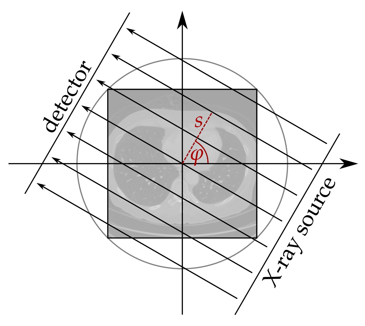
Figure 1. Parallel beam geometry. Adopted from [34].
Jimaging 07 00044 g001
Figure 2. The angular sampling ranges employed for sparse image reconstructions for (a) 50 (full), (b) 10 (subset of 50 angles), (c) 5 (subset of 50 angles) and (d) 2 angles (subset of 10 angles). The black arrows show the position of the X-ray source (dot) and the position of the detector (arrowhead). For the sparse-angle scenario, the unused angles are shown in light gray.
Jimaging 07 00044 g002
Figure 3. A horizontal cross-section of a healthy slice in an apple is shown on the left, and another cross-section with the bitter pit defects in the same apple on the right.
Jimaging 07 00044 g003
Figure 4. Reconstructions on the challenge set from the LoDoPaB-CT dataset. The window [ 0 , 0.45 ] corresponds to a HU range of ≈[−1001, 831] .
Jimaging 07 00044 g004
Figure 5. Mean data discrepancy Pois between the noisy measurements and the forward-projected reconstructions, respectively the noise-free measurements. Evaluation is done on the LoDoPaB challenge images.
Jimaging 07 00044 g005
Figure 6. Visual overview of one apple slice with bitter pit for different learned methods. Evaluated on Gaussian noise. The quality of the reconstruction deteriorates very quickly for a reduced number of angles. For the 2-angle case, none of the methods can reconstruct the exact shape of the apple.
Jimaging 07 00044 g006
Figure 7. Mean squared error (MSE) data discrepancy between the measurements and the forward-projected reconstructions for the noise-free (left) and Gaussian noise (right) dataset. The MSE values are plotted against the number of angles used for the reconstruction. For the Gaussian dataset, the mean data discrepancy between noisy and noise-free measurements is given for reference. Evaluation is done on 100 Apple CT test images. See Table A6 for the exact values.
Jimaging 07 00044 g007
Table 1. Settings of the low-dose parallel beam computed tomography (LoDoPaB-CT) and Apple CT datasets.
PropertyLoDoPaB-CTApple CT
SubjectHuman thoraxApples
Scenariolow photon countsparse-angle
Challenge3678 reconstructions100 reconstructions
Image size 362   px × 362   px 972   p x × 972   p x
Angles100050, 10, 5, 2
Detector bins5131377
Sampling ratio≈3.9≈0.07– 0.003
Table 2. Results on the LoDoPaB-CT challenge set. Methods are ranked by their overall performance. The highest value for each metric is highlighted. All values are taken from the official challenge leaderboard https://lodopab.grand-challenge.org/evaluation/challenge/leaderboard/ (accessed on 4 January 2021).
ModelPSNRPSNR-FRSSIMSSIM-FRNumber of Parameters
Learned P.-D.36.25 ± 3.7040.52 ± 3.640.866 ± 0.1150.926 ± 0.076874,980
ISTA U-Net36.09 ± 3.6940.36 ± 3.650.862 ± 0.1200.924 ± 0.08083,396,865
U-Net36.00 ± 3.6340.28 ± 3.590.862 ± 0.1190.923 ± 0.079613,322
MS-D-CNN35.85 ± 3.6040.12 ± 3.560.858 ± 0.1220.921 ± 0.082181,306
U-Net++35.37 ± 3.3639.64 ± 3.400.861 ± 0.1190.923 ± 0.0809,170,079
CINN35.54 ± 3.5139.81 ± 3.480.854 ± 0.1220.919 ± 0.0816,438,332
DIP + TV34.41 ± 3.2938.68 ± 3.290.845 ± 0.1210.913 ± 0.082hyperp.
iCTU-Net33.70 ± 2.8237.97 ± 2.790.844 ± 0.1200.911 ± 0.081147,116,792
TV33.36 ± 2.7437.63 ± 2.700.830 ± 0.1210.903 ± 0.082(hyperp.)
FBP30.19 ± 2.5534.46 ± 2.180.727 ± 0.1270.836 ± 0.085(hyperp.)
Table 3. Mean and standard deviation of data discrepancy Pois . Evaluation is done on the LoDoPaB challenge images.
Method Pois ( A x ^ | y δ ) / 10 9
Learned Primal-Dual 4.022182 ± 0.699460
ISTA U-Net 4.022185 ± 0.699461
U-Net 4.022185 ± 0.699460
MS-D-CNN 4.022182 ± 0.699460
U-Net++ 4.022163 ± 0.699461
CINN 4.022184 ± 0.699460
DIP + TV 4.022183 ± 0.699466
iCTU-Net 4.022038 ± 0.699430
TV 4.022189 ± 0.699463
FBP 4.021595 ± 0.699282
Pois ( A x | y δ ) / 10 9
Ground truth 4.022184 ± 0.699461
Table 4. Peak signal-to-noise ratio (PSNR) and structural similarity (SSIM) (adapted to the data range of each ground truth image) for the different noise settings on the Apple CT datasets. Best results are highlighted in gray. See Figure A7 and Figure A1 for a visualization.
Noise-FreePSNRSSIM
Number of Angles501052501052
Learned Primal-Dual38.7235.8530.7922.000.9010.8700.8270.740
ISTA U-Net38.8634.5428.3120.480.8970.8540.7970.686
U-Net39.6233.5127.7719.780.9130.8030.8030.676
MS-D-CNN39.8534.3828.4520.550.9130.8370.7760.646
CINN39.5934.8427.8119.460.9130.8710.7620.674
iCTU-Net36.0729.9525.6319.280.8780.8470.8240.741
TV39.2729.0022.0415.950.9150.7830.6070.661
CGLS33.0521.8112.6015.250.7800.6190.5370.615
FBP30.3917.0915.5113.970.7140.5840.4800.438
Gaussian NoisePSNRSSIM
Number of Angles501052501052
Learned Primal-Dual36.6233.7629.9221.410.8780.8500.8210.674
ISTA U-Net36.0433.5528.4820.710.8710.8510.8110.690
U-Net36.4832.8327.8019.860.8820.8180.7890.706
MS-D-CNN36.6733.2027.9819.880.8830.8310.7480.633
CINN36.7731.8826.5719.990.8880.7710.7220.637
iCTU-Net32.9029.7624.6719.440.8480.8370.8010.747
TV32.3627.1221.8316.080.8330.7520.6220.637
CGLS27.3621.0914.9015.110.7670.6240.5530.616
FBP27.8817.0915.5113.970.6950.5830.4800.438
Scattering NoisePSNRSSIM
Number of Angles501052501052
Learned Primal-Dual37.8034.1927.0820.980.8920.8660.7960.540
ISTA U-Net35.9432.3327.4119.950.8810.8200.7630.676
U-Net34.9632.9126.9318.940.8300.7840.7360.688
MS-D-CNN38.0433.5127.7320.190.8990.8180.7570.635
CINN38.5634.0828.0419.140.9150.8630.8390.754
iCTU-Net26.2622.8521.2518.320.8380.7960.7920.765
TV21.0920.1417.8614.530.7890.6490.5310.611
CGLS20.8418.2814.0214.180.7890.6180.5470.625
FBP21.0115.8014.2613.060.7540.5730.4750.433
Table 5. Performance of a U-Net trained on the Apple CT dataset (scattering noise) and evaluated on different angular samplings. In general, a U-Net trained on a specific number of angles fails to produce good results on a different number of angles. PSNR and SSIM are calculated with image-dependent data range.
Evaluation50 Angles10 Angles5 Angles2 Angles
TrainingPSNRSSIMPSNRSSIMPSNRSSIMPSNRSSIM
50 angles39.620.91316.390.45711.930.3598.7600.252
10 angles27.590.68933.510.80318.440.6079.2200.394
5 angles24.510.70826.190.73627.770.80311.850.549
2 angles15.570.48714.590.44015.940.51419.780.676
Table 6. Summary of selected reconstruction method features. The reconstruction error ratings reflect the average performance improvement in terms of the evaluated metrics PSNR and SSIM compared to filtered back-projection (FBP). Specifically, for LoDoPaB-CT improvement quotients are calculated for PSNR and SSIM, and the two are averaged; for the Apple CT experiments the quotients are determined by first averaging PSNR and SSIM values within each noise setting over the four angular sampling cases, next computing improvement quotients independently for all three noise settings and for PSNR and SSIM, and finally averaging over these six quotients. GPU memory values are compared for 1-sample batches.
ModelReconstruction
Error (Image Metrics)
Training
Time
Recon-
Struction
Time
GPU
Memory
Learned
Para-
Meters
Uses D Y
Discre-
Pancy
Operator
Required
Learned P.-D. 🟉 🟉 🟉 🟉 🟉 🟉 🟉 🟉 🟉 🟉 🟉 🟉 🟉 🟉 🟉 no 🟉 🟉 🟉
ISTA U-Net 🟉 🟉 🟉 🟉 🟉 🟉 🟉 🟉 🟉 🟉 🟉 🟉 🟉 🟉 no 🟉 🟉
U-Net 🟉 🟉 🟉 🟉 🟉 🟉 🟉 🟉 🟉 🟉 🟉 no 🟉 🟉
MS-D-CNN 🟉 🟉 🟉 🟉 🟉 🟉 🟉 🟉 🟉 🟉 🟉 🟉 no 🟉 🟉
U-Net++ 🟉 🟉 - 🟉 🟉 🟉 🟉 🟉 🟉 🟉 🟉 🟉 🟉 no 🟉 🟉
CINN 🟉 🟉 🟉 🟉 🟉 🟉 🟉 🟉 🟉 🟉 🟉 🟉 🟉 🟉 no 🟉 🟉
DIP + TV 🟉 🟉 🟉 -- 🟉 🟉 🟉 🟉 🟉 🟉 3+yes 🟉 🟉 🟉 🟉
iCTU-Net 🟉 🟉 🟉 🟉 🟉 🟉 🟉 🟉 🟉 🟉 🟉 🟉 🟉 🟉 🟉 🟉 no 🟉
TV 🟉 🟉 🟉 🟉 🟉 🟉 - 🟉 🟉 🟉 🟉 3yes 🟉 🟉 🟉 🟉
CGLS- 🟉 🟉 🟉 🟉 - 🟉 🟉 1yes 🟉 🟉 🟉 🟉
FBP 🟉 🟉 🟉 🟉 🟉 🟉 🟉 🟉 - 🟉 🟉 2no 🟉 🟉 🟉 🟉
LegendLoDoPaBApple CTRough values for Apple CT Dataset B
Avg. improv. over FBP(varying for different setups and datasets)
🟉 🟉 🟉 🟉 0%0–15%>2 weeks>10 min>10 GiB> 10 8 Direct
🟉 🟉 🟉 12–16%25–30%>5 days>30 s>3 GiB> 10 6 In network
🟉 🟉 17–20%40–45%>1 day>0.1 s>1.5 GiB> 10 5 For input
🟉 50–60% ≤0.02 s≤1 GiB 10 5 Only concept
Publisher’s Note: MDPI stays neutral with regard to jurisdictional claims in published maps and institutional affiliations.