
Colour and Texture Descriptors for Visual Recognition: A Historical Overview


Abstract
:1. Introduction
2. Colour and Texture Descriptors for Visual Recognition: Definitions, Taxonomy and Periodisation
2.1. Colour and Texture
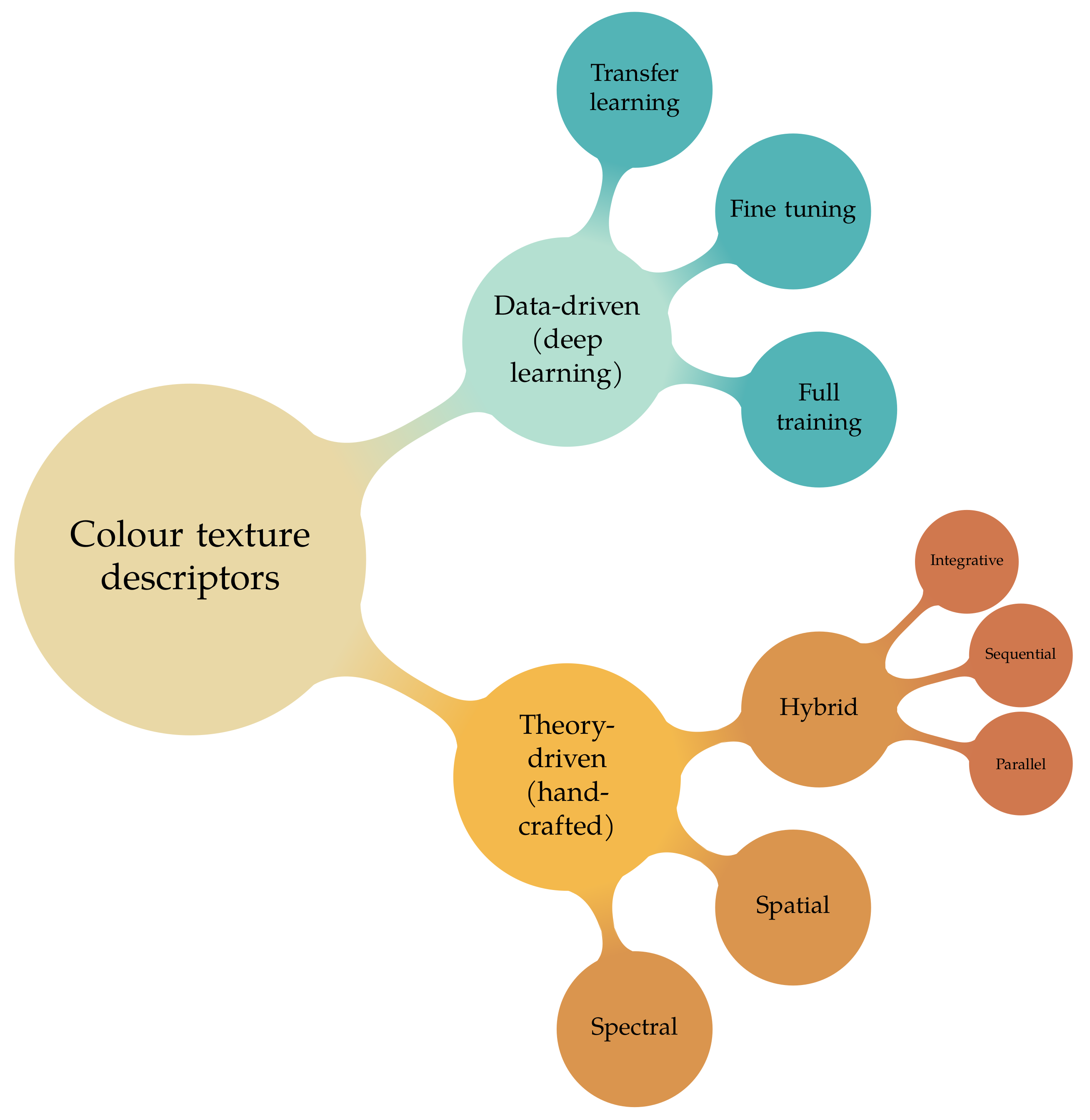
2.2. Taxonomy
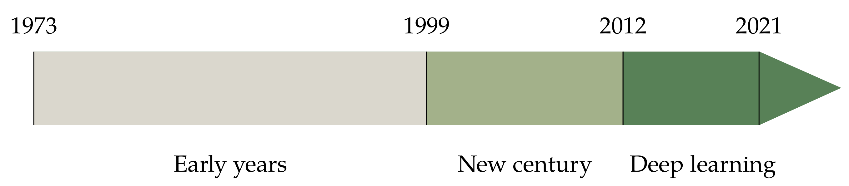
2.3. Periodisation
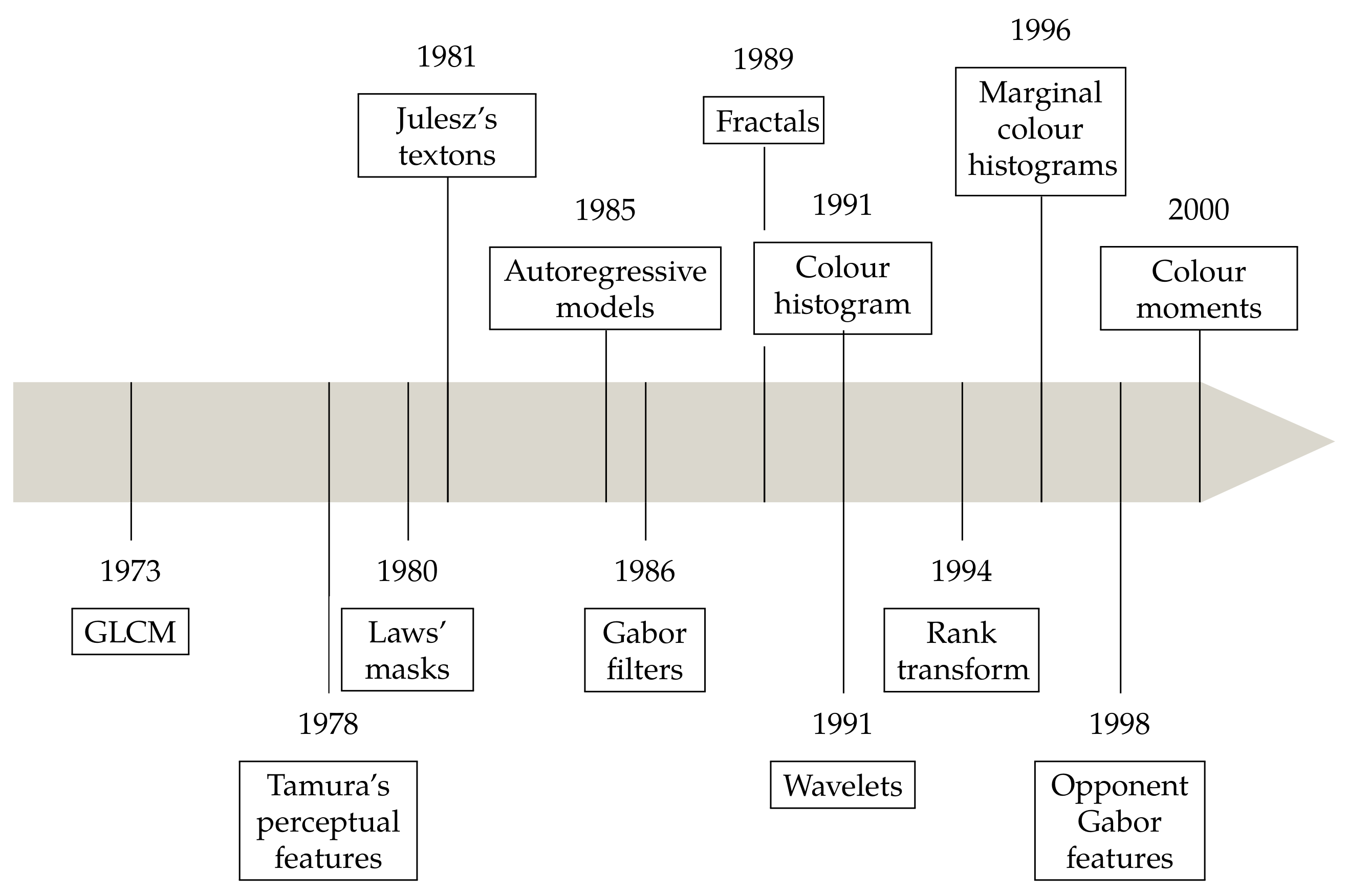
3. The Early Years
3.1. Spatial Descriptors
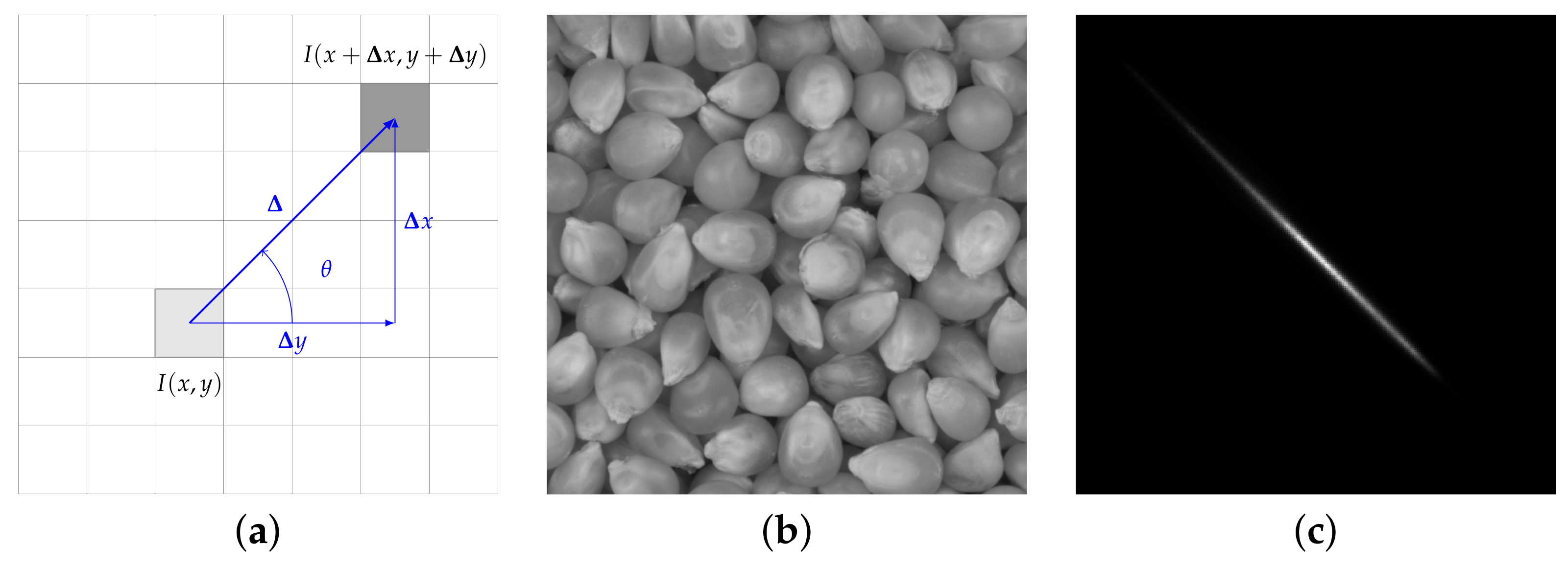
3.1.1. Grey-Level Co-Occurrence Matrices
3.1.2. Tamura’s Perceptual Features
3.1.3. Autoregressive Models
3.1.4. Fractals
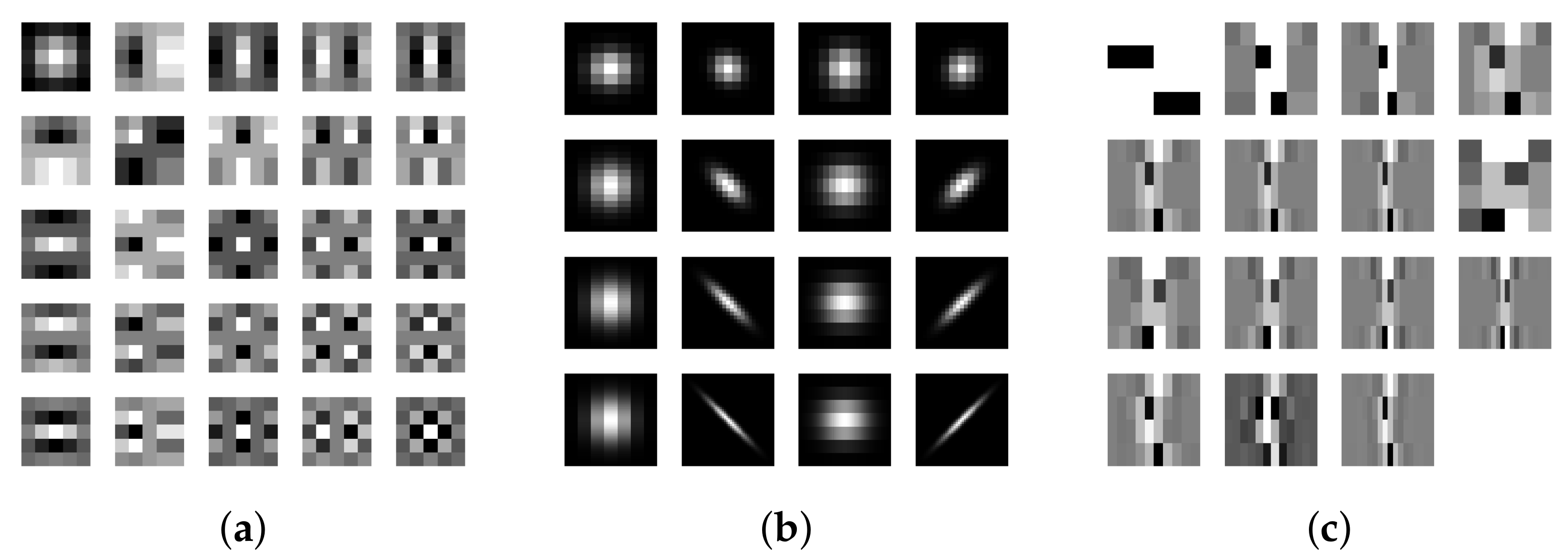
3.1.5. Filtering
Laws’ Masks
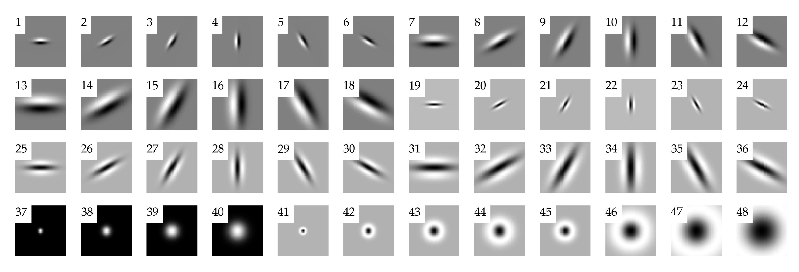
Gabor Filters
Wavelets
3.2. Julesz’s Textons
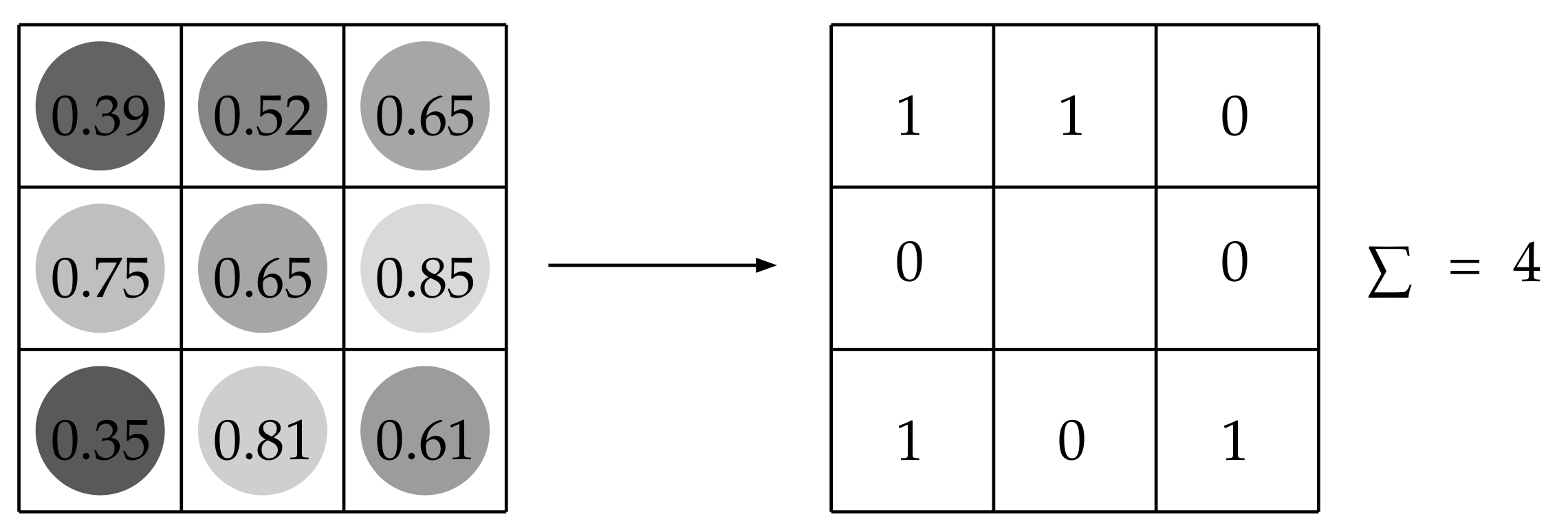
3.3. Rank Transform
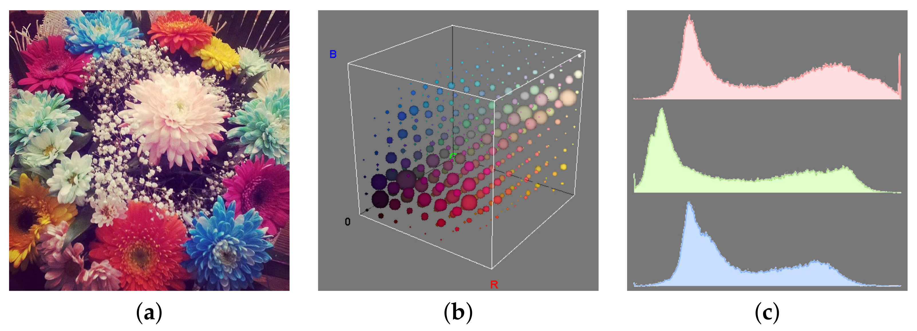
3.4. Spectral Methods
3.4.1. Colour Histogram
3.4.2. Marginal Histograms
3.4.3. Colour Moments
3.5. Hybrid Methods
Opponent Gabor Features
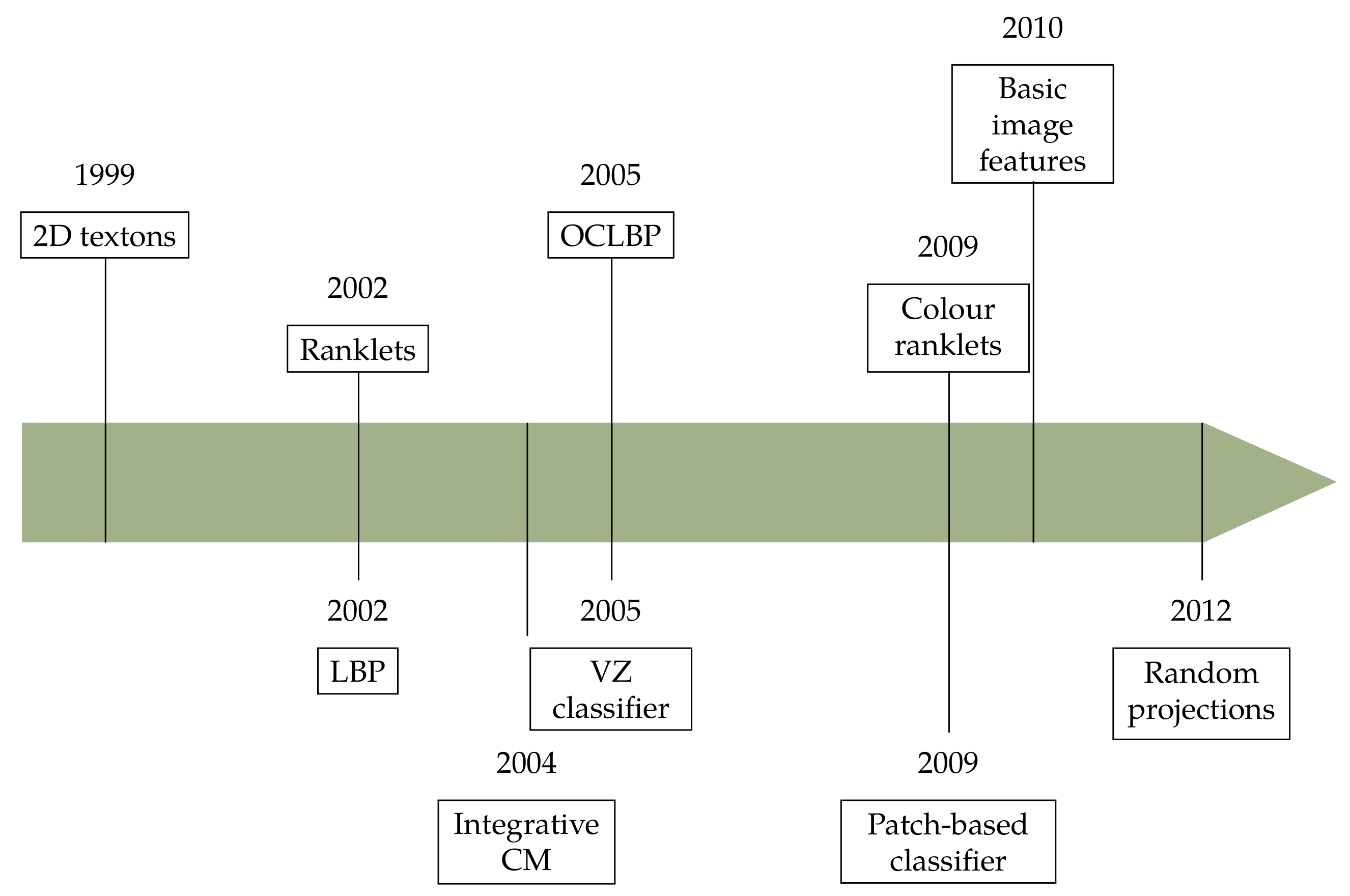
4. The New Century
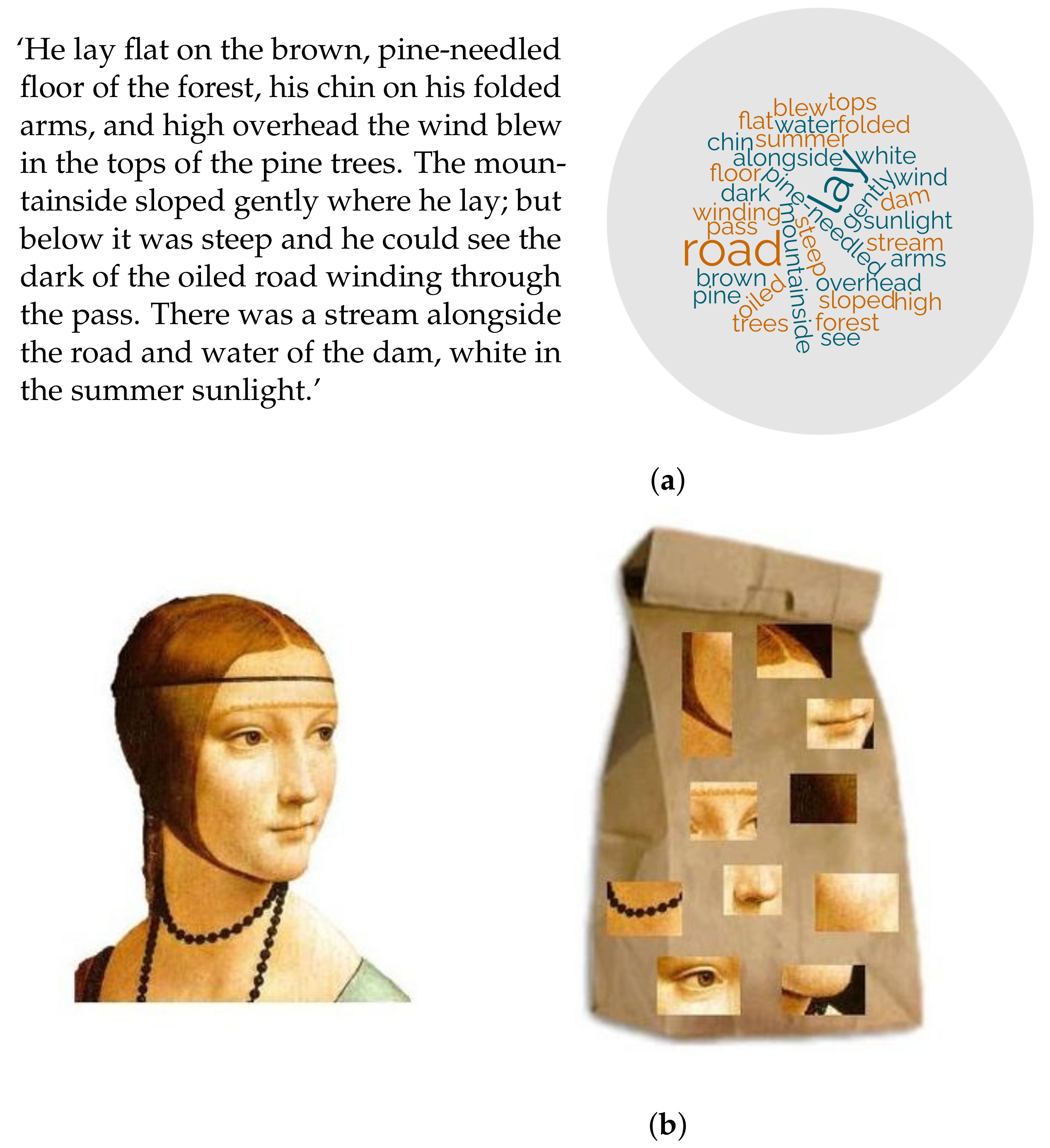
4.1. The Bag-of-Visual-Words Model
4.2. Spatial Methods
4.2.1. BoVW
Two-Dimensional Textons
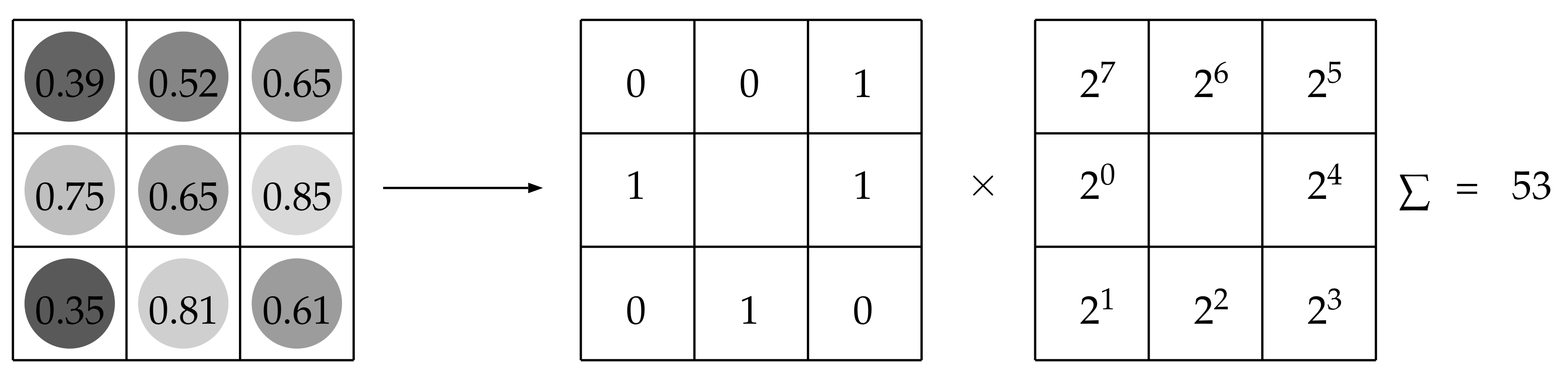
Local Binary Patterns
VZ Classifier
Image Patch-Based Classifier
Basic Image Features
Random Projections
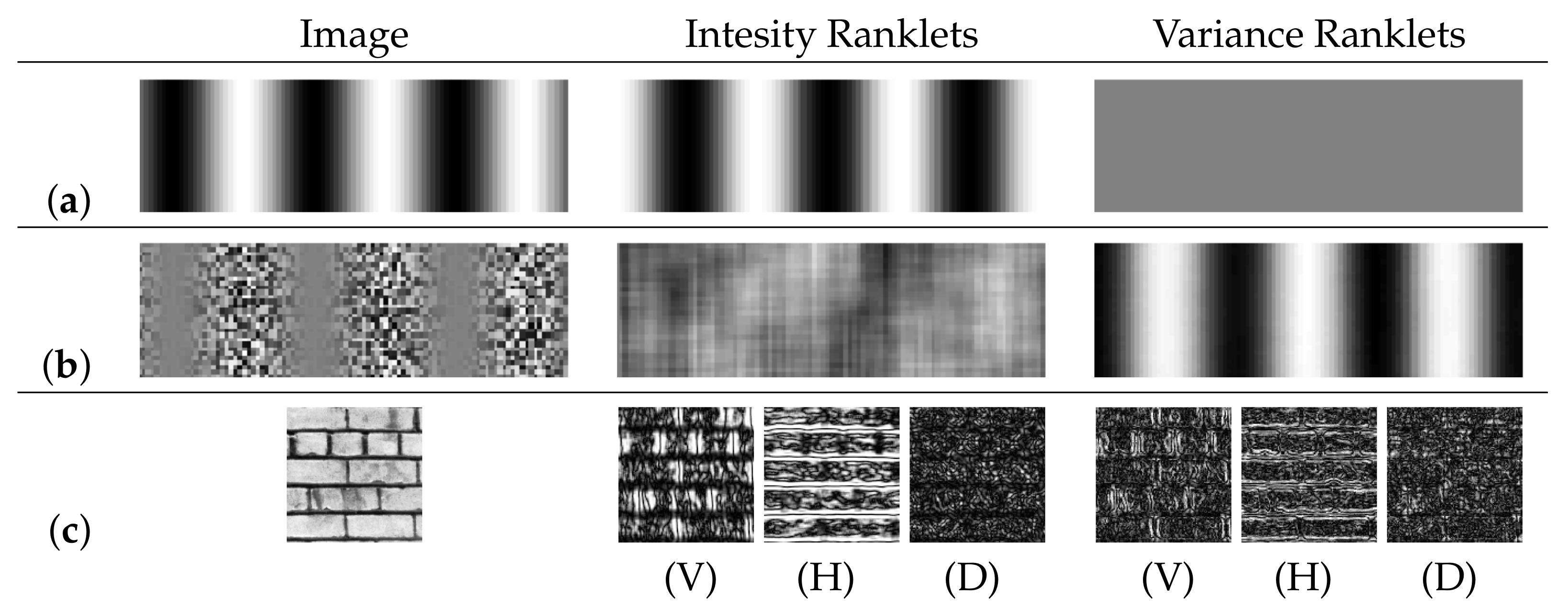
4.2.2. Ranklets
4.3. Hybrid Methods
4.3.1. Integrative Co-Occurrence Matrices
4.3.2. Opponent-Colour Local Binary Patterns
5. Deep Learning
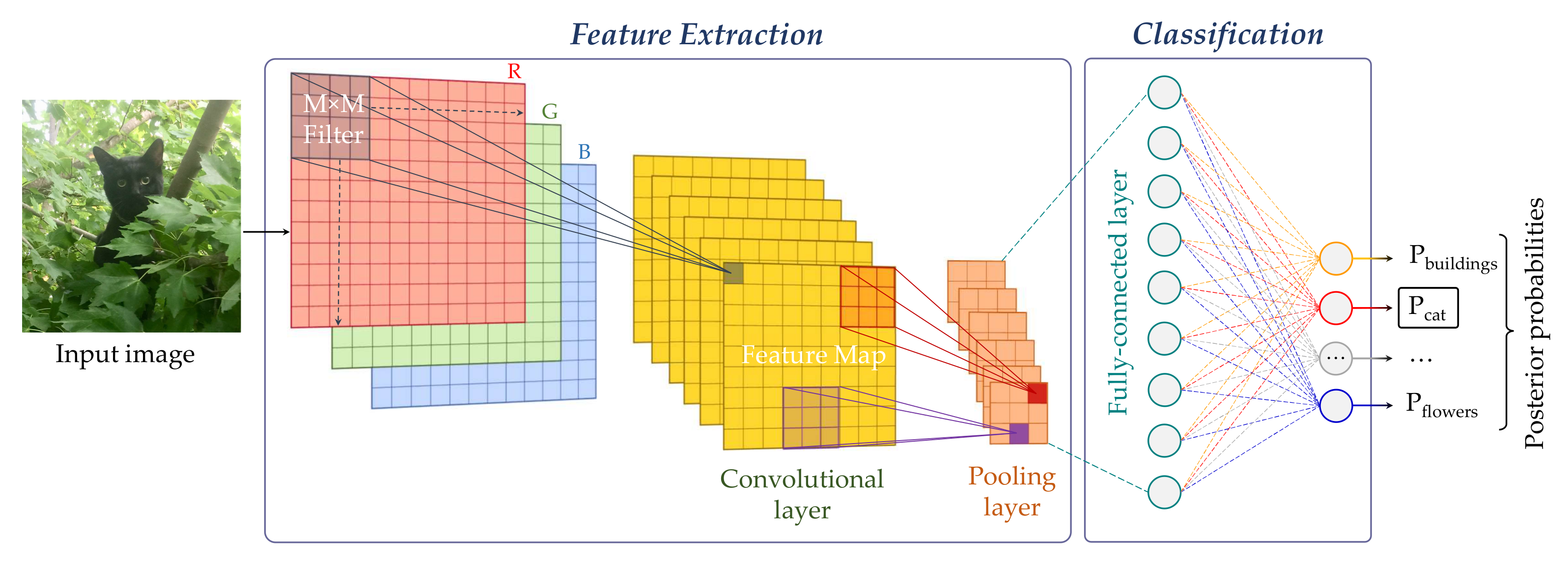
5.1. Basic CNN Blocks
5.1.1. Convolutional Layers
5.1.2. Pooling Layers
5.1.3. Fully-Connected Layers
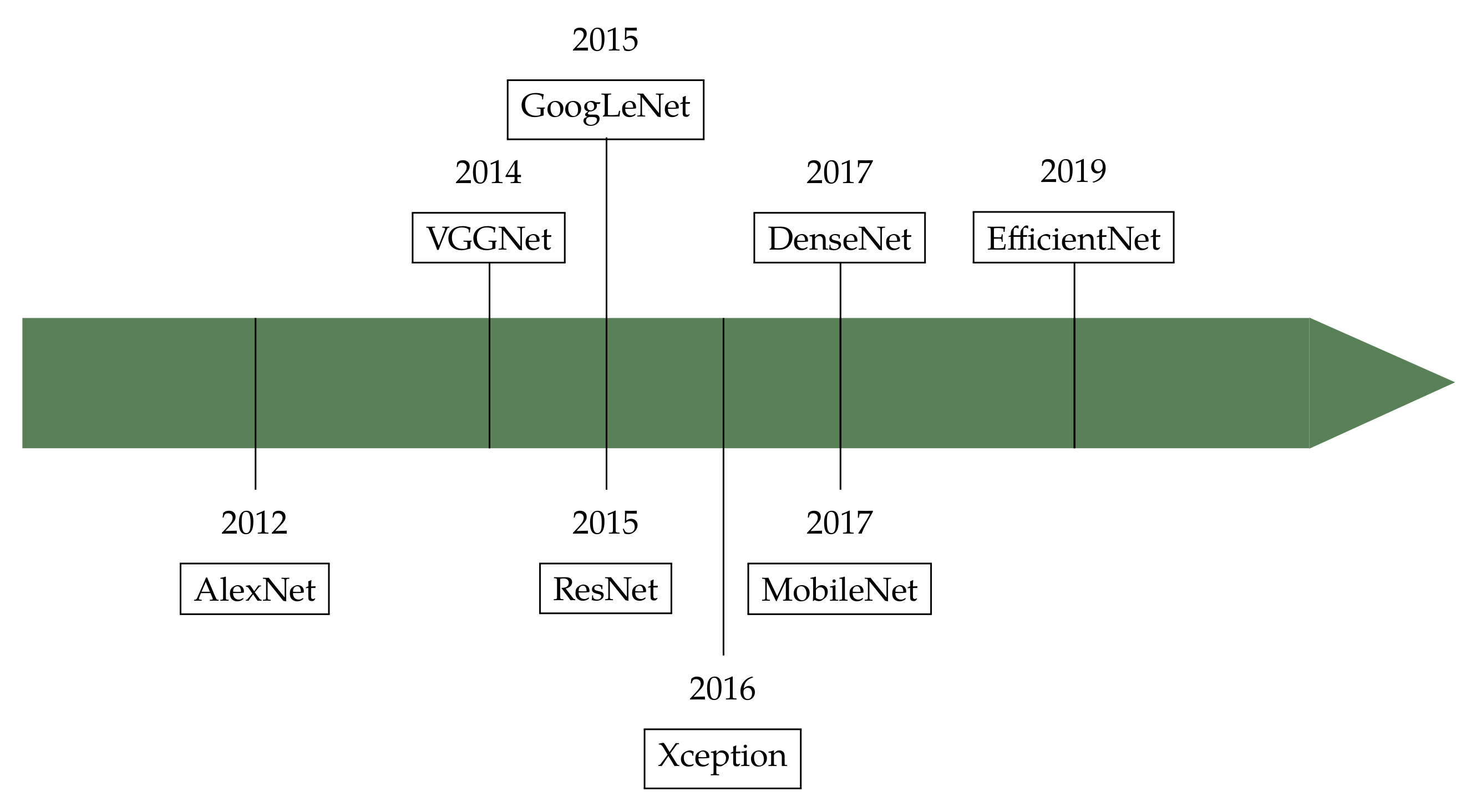
5.2. Architectures
5.2.1. AlexNet
5.2.2. VGGNet
5.2.3. GoogLeNet
5.2.4. Residual Networks (ResNets)
5.2.5. Densely Connected Networks (DenseNets)
5.2.6. MobileNets
5.2.7. EfficientNets
5.3. Usage
CNNs for Colour Texture Classification
6. Discussion
7. Conclusions
Author Contributions
Funding
Institutional Review Board Statement
Informed Consent Statement
Data Availability Statement
Conflicts of Interest
Abbreviations
| BIF | Basic Image Features |
| BoVW | Bag of Visual Words |
| BoW | Bag of Words |
| CIE | Commission Internationale de l’Éclairage |
| CNN | Convolutional Neural Network(s) |
| FV | Fisher Vector |
| GLCM | Grey-Level Co-occurrence Matrices |
| ICM | Integrative Co-occurrence Matrices |
| IPBC | Image Patch-Based Classifier |
| OCLBP | Opponent-Colour Local Binary Patterns |
| LBP | Local Binary Patterns |
| RP | Random Projections |
| RT | Rank Transform |
| VLAD | Vectors of Locally-Aggregated Descriptors |
| XAI | Explainable Artificial Intelligence |
References
- Pam, M.S. Visual Recognition. 2013. Available online: https://psychologydictionary.org/visual-recognition/ (accessed on 20 May 2021).
- Oxford English Dictionary. Online Version. 2020. Available online: https://www.oed.com/ (accessed on 20 May 2021).
- Wyszecki, G.; Stiles, W.S. Color Science. Concepts and Methods, Quantitative Data and Formulae, 2nd ed.; John Wiley & Sons: New York, NY, USA, 1982. [Google Scholar]
- Kang, H.R. Computational Color Technology; SPIE Press: Bellingham, WA, USA, 2006. [Google Scholar]
- Khelifi, R.; Adel, M.; Bourennane, S. Texture classification for multi-spectral images using spatial and spectral gray level differences. In Proceedings of the 2nd International Conference on Image Processing Theory, Tools and Applications, Paris, France, 7–10 July 2010; pp. 330–333. [Google Scholar]
- Khelifi, R.; Adel, M.; Bourennane, S. Multispectral texture characterization: Application to computer aided diagnosis on prostatic tissue images. Eurasip J. Adv. Signal Process. 2012, 2012, 118. [Google Scholar] [CrossRef] [Green Version]
- Kupidura, P. The comparison of different methods of texture analysis for their efficacy for land use classification in satellite imagery. Remote Sens. 2019, 11, 1233. [Google Scholar] [CrossRef] [Green Version]
- Vandenbroucke, N.; Porebski, A. Multi color channel vs. Multi spectral band representations for texture classification. In Proceedings of the 25th International Conference on Pattern Recognition Workshops, Milan, Italy, 10–15 January 2020; Volume 12662, pp. 310–324. [Google Scholar]
- Conni, M.; Nussbaum, P.; Green, P. The effect of camera calibration on multichannel texture classification. J. Imaging Sci. Technol. 2021, 65, 010503. [Google Scholar] [CrossRef]
- Bigun, J. Vision with Direction: A Systematic Introduction to Image Processing and Computer Vision; Springer: Heidelberg, Germany, 2006. [Google Scholar]
- Hung, C.C.; Song, E.; Lan, Y. Image Texture Analysis: Foundations, Models and Algorithms; Springer: Cham, Switzerland, 2019. [Google Scholar]
- Davies, R. Introduction to Texture Analysis. In Handbook of Texture Analysis; Mirmehdi, M., Xie, X., Suri, J., Eds.; Imperial College Press: London, UK, 2008; pp. 1–31. [Google Scholar]
- Paget, R. Texture Modelling and Synthesis. In Handbook of Texture Analysis; Mirmehdi, M., Xie, X., Suri, J., Eds.; Imperial College Press: London, UK, 2008; pp. 33–60. [Google Scholar]
- Petrou, M.; García Sevilla, P. Image Processing. Dealing with Texture; John Wiley & Sons: New York, NY, USA, 2006. [Google Scholar]
- Haralick, R.M. Statistical and structural approaches to texture. Proc. IEEE 1979, 67, 786–804. [Google Scholar] [CrossRef]
- Tuceryan, M.; Jain, A.K. Texture analysis. In Handbook of Pattern Recognition & Computer Vision; Chen, C.H., Pau, L.F., Wang, P.S.P., Eds.; World Scientific Publishing: River Edge, NJ, USA, 1993; pp. 235–276. [Google Scholar]
- Sonka, M.; Hlavac, V.; Boyle, R. Image Processing, Analysis and Machine Vision; Chapman & Hall: London, UK, 1993. [Google Scholar]
- Bergman, R.; Nachlieli, H.; Ruckenstein, G. Detection of textured areas in natural images using an indicator based on component counts. J. Electron. Imaging 2008, 17, 043003. [Google Scholar] [CrossRef]
- Xie, X.; Mirmehdi, M. A Galaxy of Texture Features. In Handbook of Texture Analysis; Mirmehdi, M., Xie, X., Suri, J., Eds.; Imperial College Press: London, UK, 2008; pp. 375–406. [Google Scholar]
- Palm, C. Color texture classification by integrative Co-occurrence matrices. Pattern Recognit. 2004, 37, 965–976. [Google Scholar] [CrossRef]
- Bianconi, F.; Harvey, R.; Southam, P.; Fernández, A. Theoretical and experimental comparison of different approaches for color texture classification. J. Electron. Imaging 2011, 20, 043006. [Google Scholar] [CrossRef]
- Liu, L.; Fieguth, P.; Guo, Y.; Wang, X.; Pietikäinen, M. Local binary features for texture classification: Taxonomy and experimental study. Pattern Recognit. 2017, 62, 135–160. [Google Scholar] [CrossRef] [Green Version]
- Liu, L.; Chen, J.; Fieguth, P.; Zhao, G.; Chellappa, R.; Pietikäinen, M. From BoW to CNN: Two decades of Texture Representation for Texture Classification. Int. J. Comput. Vis. 2019, 127, 74–109. [Google Scholar] [CrossRef] [Green Version]
- Humeau-Heurtier, A. Texture feature extraction methods: A survey. IEEE Access 2019, 7, 8975–9000. [Google Scholar] [CrossRef]
- Bello-Cerezo, R.; Bianconi, F.; Di Maria, F.; Napoletano, P.; Smeraldi, F. Comparative Evaluation of Hand-Crafted Image Descriptors vs. Off-the-Shelf CNN-Based Features for Colour Texture Classification under Ideal and Realistic Conditions. Appl. Sci. 2019, 9, 738. [Google Scholar] [CrossRef] [Green Version]
- Chollet, F. Deep Learning with Python; Manning: Shelter Island, NY, USA, 2018. [Google Scholar]
- González, E.; Bianconi, F.; Álvarez, M.X.; Saetta, S.A. Automatic characterization of the visual appearance of industrial materials through colour and texture analysis: An overview of methods and applications. Adv. Opt. Technol. 2013, 2013, 503541. [Google Scholar] [CrossRef] [Green Version]
- Haralick, R.M.; Shanmugam, K.; Dinstein, I. Textural Features for Image Classification. IEEE Trans. Syst. Man Cybern. 1973, 3, 610–621. [Google Scholar] [CrossRef] [Green Version]
- Krizhevsky, A.; Sutskever, I.; Hinton, G.E. ImageNet classification with deep convolutional neural networks. In Proceedings of the 26th Annual Conference on Neural Information Processing Systems, Lake Tahoe, NV, USA, 3–6 December 2012. [Google Scholar]
- Malik, J.; Belongie, S.; Shi, J.; Leung, T. Textons, contours and regions: Cue integration in image segmentation. In Proceedings of the IEEE International Conference on Computer Vision, Kerkyra, Greece, 20–25 September 1999; Volume 2, pp. 918–925. [Google Scholar]
- Leung, T.; Malik, J. Representing and recognizing the visual appearance of materials using three-dimensional textons. Int. J. Comput. Vis. 2001, 43, 29–44. [Google Scholar] [CrossRef]
- Ojala, T.; Pietikäinen, M.; Mäenpää, T. Multiresolution gray-scale and rotation invariant texture classification with local binary patterns. IEEE Trans. Pattern Anal. Mach. Intell. 2002, 24, 971–987. [Google Scholar] [CrossRef]
- Swain, M.J.; Ballard, D.H. Color indexing. Int. J. Comput. Vis. 1991, 7, 11–32. [Google Scholar] [CrossRef]
- Daugman, J.G. Complete Discrete 2-D Gabor Transforms by Neural Networks for Image Analysis and Compression. IEEE Trans. Acoust. Speech Signal Process. 1988, 36, 1169–1179. [Google Scholar] [CrossRef] [Green Version]
- Daubechies, I. Ten Lectures on Wavelets; CBMS-NSF Regional Conference Series in Applied Mathematics; Society for Industrial and Applied Mathematics: Philadelphia, PA, USA, 1992; Volume 61. [Google Scholar]
- Jain, A.; Healey, G. A Multiscale Representation Including Opponent Color Features for Texture Recognition. IEEE Trans. Image Process. 1998, 7, 124–128. [Google Scholar] [CrossRef] [Green Version]
- Thiyaneswaran, B.; Anguraj, K.; Kumarganesh, S.; Thangaraj, K. Early detection of melanoma images using gray level co-occurrence matrix features and machine learning techniques for effective clinical diagnosis. Int. J. Imaging Syst. Technol. 2021, 31, 682–694. [Google Scholar] [CrossRef]
- Peixoto, S.; Filho, P.P.R.; Arun Kumar, N.; de Albuquerque, V.H.C. Automatic classification of pulmonary diseases using a structural co-occurrence matrix. Neural Comput. Appl. 2020, 32, 10935–10945. [Google Scholar] [CrossRef]
- Dhanalakshmi, P.; Satyavathy, G. Grey level co-occurrence matrix (GLCM) and multi-scale non-negative sparse coding for classification of medical images. Ournal Adv. Res. Dyn. Control. Syst. 2019, 11, 481–493. [Google Scholar] [CrossRef]
- Hong, H.; Zheng, L.; Pan, S. Computation of gray level Co-Occurrence matrix based on CUDA and optimization for medical computer vision application. IEEE Access 2018, 6, 67762–67770. [Google Scholar] [CrossRef]
- Galloway, M.M. Texture analysis using gray level run lengths. Comput. Graph. Image Process. 1975, 4, 172–179. [Google Scholar] [CrossRef]
- Weszka, J.S.; Dyer, C.R.; Rosenfeld, A. A Comparative Study of Texture Measures for Terrain Classification. IEEE Trans. Syst. Man Cybern. 1976, SMC-6, 269–285. [Google Scholar] [CrossRef]
- Sun, C.; Wee, W.G. Neighboring gray level dependence matrix for texture classification. Comput. Vision Graph. Image Process. 1983, 23, 341–352. [Google Scholar] [CrossRef]
- Adamasun, M.; King, R. Textural features corresponding to textural properties. IEEE Trans. Syst. Man Cybern. 1989, 19, 1264–1274. [Google Scholar] [CrossRef]
- Cusano, C.; Napoletano, P.; Schettini, R. Evaluating color texture descriptors under large variations of controlled lighting conditions. J. Opt. Soc. Am. A Opt. Image Sci. Vis. 2016, 33, 17–30. [Google Scholar] [CrossRef] [Green Version]
- RawFooT DB: Raw Food Texture Database. Available online: http://projects.ivl.disco.unimib.it/minisites/rawfoot/ (accessed on 8 June 2021).
- Tamura, H.; Mori, T.; Yamawaki, T. Textural Features Corresponding to Visual Perception. IEEE Trans. Syst. Man Cybern. 1978, 8, 460–473. [Google Scholar] [CrossRef]
- Liu, J.; Lughofer, E.; Zeng, X. Aesthetic perception of visual textures: A holistic exploration using texture analysis, psychological experiment, and perception modeling. Front. Comput. Neurosci. 2015, 9, A134. [Google Scholar] [CrossRef] [Green Version]
- Thumfart, S.; Jacobs, R.H.A.H.; Lughofer, E.; Eitzinger, C.; Cornelissen, F.W.; Groissboeck, W.; Richter, R. Modeling human aesthetic perception of visual textures. ACM Trans. Appl. Percept. 2011, 8, 27. [Google Scholar] [CrossRef]
- Martínez-Jiménez, P.M.; Chamorro-Martínez, J.; Soto-Hidalgo, J.M. Perception-based fuzzy partitions for visual texture modeling. Fuzzy Sets Syst. 2018, 337, 1–24. [Google Scholar] [CrossRef]
- Chellappa, R.; Kashyap, R.L. Texture Synthesis Using 2-D Noncausal Autoregressive Models. IEEE Trans. Acoust. Speech Signal Process. 1985, 33, 194–203. [Google Scholar] [CrossRef]
- Mao, J.; Jain, A.K. Texture classification and segmentation using multiresolution simultaneous autoregressive models. Pattern Recognit. 1992, 25, 173–188. [Google Scholar] [CrossRef]
- Keller, J.M.; Chen, S.; Crownover, R.M. Texture description and segmentation through fractal geometry. Comput. Vision Graph. Image Process. 1989, 45, 150–166. [Google Scholar] [CrossRef]
- Varma, M.; Garg, R. Locally invariant fractal features for statistical texture classification. In Proceedings of the 11th International Conference on Computer Vision, Rio de Janeiro, Brazil, 14–21 October 2007. [Google Scholar]
- Xu, Y.; Ji, H.; Fermüller, C. Viewpoint invariant texture description using fractal analysis. Int. J. Comput. Vis. 2009, 83, 85–100. [Google Scholar] [CrossRef]
- Backes, A.R.; Casanova, D.; Bruno, O.M. Color texture analysis based on fractal descriptors. Pattern Recognit. 2012, 45, 1984–1992. [Google Scholar] [CrossRef]
- Randen, T.; Husøy, J. Filtering for Texture Classification: A Comparative Study. IEEE Trans. Pattern Anal. Mach. Intell. 1999, 21, 291–310. [Google Scholar] [CrossRef] [Green Version]
- Laws, K.I. Rapid Texture Identification. In Image Processing for Missile Guidance; Wiener, T., Ed.; SPIE: Wallisellen, Switzerland, 1980; Volume 0238. [Google Scholar]
- Daugman, J.G. Uncertainty relation for resolution in space, spatial frequency, and orientation optimized by two-dimensional visual cortical filters. J. Opt. Soc. Am. A Opt. Image Sci. Vis. 1985, 2, 1160–1169. [Google Scholar] [CrossRef]
- Franceschiello, B.; Sarti, A.; Citti, G. A Neuromathematical Model for Geometrical Optical Illusions. J. Math. Imaging Vis. 2018, 60, 94–108. [Google Scholar] [CrossRef] [Green Version]
- Clark, M.; Bovik, A.; Geisler, W.S. Texture segmentation using Gabor modulation/demodulation. Pattern Recognit. Lett. 1987, 6, 261–267. [Google Scholar] [CrossRef]
- Jain, A.; Farrokhnia, F. Unsupervised texture segmentation using Gabor filters. Pattern Recognit. 1991, 24, 1167–1186. [Google Scholar] [CrossRef] [Green Version]
- Grossmann, A.; Morlet, J. Decomposition of Hardy functions into square integrable wavelets of constant shape. SIAM J. Math. Anal. 1984, 15, 723–736. [Google Scholar] [CrossRef]
- Carter, P.H. Texture discrimination using wavelets. In Applications of Digital Image Processing XIV; Society of Photo-Optical Instrumentation Engineers (SPIE): San Diego, CA, USA, 1991; Volume 1567. [Google Scholar]
- Unser, M. Texture discrimination using wavelets. IEEE Trans. Image Process. 1995, 4, 1549–1560. [Google Scholar] [CrossRef] [PubMed] [Green Version]
- Greiner, T. Orthogonal and biorthogonal texture-matched wavelet filterbanks for hierarchical texture analysis. Signal Process. 1996, 54, 1–22. [Google Scholar] [CrossRef]
- Issac Niwas, S.; Palanisamy, P.; Sujathan, K.; Bengtsson, E. Analysis of nuclei textures of fine needle aspirated cytology images for breast cancer diagnosis using complex Daubechies wavelets. Signal Process. 2013, 93, 2828–2837. [Google Scholar] [CrossRef]
- Julesz, B. Textons, the elements of texture perception, and their interactions. Nature 1981, 290, 91–97. [Google Scholar] [CrossRef]
- Zabih, R.; Woodfill, J. Non-parametric local transforms for computing visual correspondence. In Proceedings of the 3rd European Conference on Computer Vision, Stockholm, Sweden, 2–6 May 1994; Lecture Notes in Computer Science. Volume 801, pp. 151–158. [Google Scholar]
- Lee, S.H.; Sharma, S. Real-time disparity estimation algorithm for stereo camera systems. IEEE Trans. Consum. Electron. 2011, 57, 1018–1026. [Google Scholar] [CrossRef]
- Díaz, J.; Ros, E.; Rodríguez-Gómez, R.; Del Pino, B. Real-time architecture for robust motion estimation under varying illumination conditions. J. Univers. Comput. Sci. 2007, 13, 363–376. [Google Scholar]
- Mäenpää, T.; Pietikäinen, M. Classification with color and texture: Jointly or separately? Pattern Recognit. 2004, 37, 1629–1640. [Google Scholar] [CrossRef] [Green Version]
- Napoletano, P. Hand-Crafted vs Learned Descriptors for Color Texture Classification. In Proceedings of the 6th Computational Color Imaging Workshop (CCIW’17), Milan, Italy, 29–31 March 2017; Lecture Notes in Computer Science. Volume 10213, pp. 259–271. [Google Scholar]
- Paschos, G. Fast color texture recognition using chromaticity moments. Pattern Recognit. Lett. 2000, 21, 837–841. [Google Scholar] [CrossRef]
- López, F.; Miguel Valiente, J.; Manuel Prats, J.; Ferrer, A. Performance evaluation of soft color texture descriptors for surface grading using experimental design and logistic regression. Pattern Recognit. 2008, 41, 1761–1772. [Google Scholar] [CrossRef]
- López, F.; Valiente, J.M.; Prats, J.M. Surface grading using soft colour-texture descriptors. In Proceedings of the CIARP 2005: Progress in Pattern Recognition, Image Analysis and Applications, Havana, Cuba, 9–12 September 2005; Lecture Notes in Computer Science (Including Subseries Lecture Notes in Artificial Intelligence and Lecture Notes in Bioinformatics). Volume 3773, pp. 13–23. [Google Scholar]
- Bianconi, F.; Fernández, A.; González, E.; Saetta, S.A. Performance analysis of colour descriptors for parquet sorting. Expert Syst. Appl. 2013, 40, 1636–1644. [Google Scholar] [CrossRef]
- Drimbarean, A.; Whelan, P. Experiments in colour texture analysis. Pattern Recognit. Lett. 2001, 22, 1161–1167. [Google Scholar] [CrossRef] [Green Version]
- Hemingway, E. For Whom the Bell Tolls; Arrow Books: London, UK, 2004. [Google Scholar]
- Brahnam, S.; Jain, L.C.; Nanni, L.; Lumini, A. (Eds.) Local Binary Patterns: New Variants and Applications; Studies in Computational Intelligence; Springer: Berlin/Heidelberg, Germany, 2014; Volume 506. [Google Scholar]
- Jégou, H.; Perronnin, F.; Douze, M.; Sánchez, J.; Pérez, P.; Schmid, C. Aggregating local image descriptors into compact codes. IEEE Trans. Pattern Anal. Mach. Intell. 2012, 34, 1704–1716. [Google Scholar] [CrossRef] [PubMed] [Green Version]
- Fernández, A.; Álvarez, M.X.; Bianconi, F. Texture description through histograms of equivalent patterns. J. Math. Imaging Vis. 2013, 45, 76–102. [Google Scholar] [CrossRef] [Green Version]
- Pardo-Balado, J.; Fernández, A.; Bianconi, F. Texture classification using rotation invariant LBP based on digital polygons. In New Trends in Image Analysis and Processing—ICIAP 2015 Workshops; Murino, V., Puppo, E., Eds.; Lecture Notes in Computer Science; Springer: Berlin/Heidelberg, Germany, 2015; Volume 9281, pp. 87–94. [Google Scholar]
- Nanni, L.; Lumini, A.; Brahnam, S. Local binary patterns variants as texture descriptors for medical image analysis. Artif. Intell. Med. 2010, 49, 117–125. [Google Scholar] [CrossRef]
- George, M.; Zwiggelaar, R. Comparative study on local binary patterns for mammographic density and risk scoring. J. Imaging 2019, 5, 24. [Google Scholar] [CrossRef] [Green Version]
- Pietikäinen, M.; Zhao, G. Two decades of local binary patterns: A survey. In Advances in Independent Component Analysis and Learning Machines; Bingham, E., Kaski, S., Laaksonen, J., Lampinen, J., Eds.; Academic Press: Amsterdam, The Netherlands, 2015; pp. 175–210. [Google Scholar]
- Varma, M.; Zisserman, A. A statistical approach to texture classification from single images. Int. J. Comput. Vis. 2005, 62, 61–81. [Google Scholar] [CrossRef]
- Varma, M.; Zisserman, A. A statistical approach to material classification using image patch exemplars. IEEE Trans. Pattern Anal. Mach. Intell. 2009, 31, 2032–2047. [Google Scholar] [CrossRef]
- Crosier, M.; Griffin, L.D. Using basic image features for texture classification. Int. J. Comput. Vis. 2010, 88, 447–460. [Google Scholar] [CrossRef] [Green Version]
- Liu, L.; Fieguth, P. Texture classification from random features. IEEE Trans. Pattern Anal. Mach. Intell. 2012, 34, 574–586. [Google Scholar] [CrossRef]
- Smeraldi, F. Ranklets: Orientation selective non-parametric features applied to face detection. In Proceedings of the 16th International Conference on Pattern Recognition (ICPR 2002), Quebec City, CA, USA, 11–15 August 2002; Volume 3, pp. 379–382. [Google Scholar]
- Azzopardi, G.; Smeraldi, F. Variance Ranklets: Orientation-selective Rank Features for Contrast Modulations. In Proceedings of the British Machine Vision Conference (BMVC), London, UK, 7–10 September 2009. [Google Scholar]
- Bianconi, F.; Fernández, A.; González, E.; Armesto, J. Robust color texture features based on ranklets and discrete Fourier transform. J. Electron. Imaging 2009, 18, 043012. [Google Scholar]
- Masotti, M.; Lanconelli, N.; Campanini, R. Computer-aided mass detection in mammography: False positive reduction via gray-scale invariant ranklet texture features. Med. Phys. 2009, 36, 311–316. [Google Scholar] [CrossRef] [PubMed]
- Yang, M.C.; Moon, W.K.; Wang, Y.C.F.; Bae, M.S.; Huang, C.S.; Chen, J.H.; Chang, R.F. Robust Texture Analysis Using Multi-Resolution Gray-Scale Invariant Features for Breast Sonographic Tumor Diagnosis. IEEE Trans. Med. Imaging 2013, 32, 2262–2273. [Google Scholar] [CrossRef] [Green Version]
- Lo, C.M.; Hung, P.H.; Hsieh, K.L.C. Computer-Aided Detection of Hyperacute Stroke Based on Relative Radiomic Patterns in Computed Tomography. Appl. Sci. 2019, 9, 1668. [Google Scholar] [CrossRef] [Green Version]
- Brodatz, P. Textures: A Photographic Album for Artists and Designers; Dover: New York, NY, USA, 1966. [Google Scholar]
- Arvis, V.; Debain, C.; Berducat, M.; Benassi, A. Generalization of the cooccurrence matrix for colour images: Application to colour texture classification. Image Anal. Stereol. 2004, 23, 63–72. [Google Scholar] [CrossRef] [Green Version]
- Losson, O.; Porebski, A.; Vandenbroucke, N.; Macaire, L. Color texture analysis using CFA chromatic co-occurrence matrices. Comput. Vis. Image Underst. 2013, 117, 747–763. [Google Scholar] [CrossRef]
- Cusano, C.; Napoletano, P.; Schettini, R. T1k+: A database for benchmarking color texture classification and retrieval methods. Sensors 2021, 21, 1010. [Google Scholar] [CrossRef]
- Mäenpää, T.; Pietikäinen, M. Texture Analysis with Local Binary Patterns. In Handbook of Pattern Recognition and Computer Vision, 3rd ed.; Chen, C.H., Wang, P.S.P., Eds.; World Scientific Publishing: River Edge, NJ, USA, 2005; pp. 197–216. [Google Scholar]
- Kather, J.N.; Bello-Cerezo, R.; Di Maria, F.; van Pelt, G.W.; Mesker, W.E.; Halama, N.; Bianconi, F. Classification of tissue regions in histopathological images: Comparison between pre-trained convolutional neural networks and local binary patterns variants. In Deep Learners and Deep Learner Descriptors for Medical Applications; Nanni, L., Brahnam, S., Brattin, R., Ghidoni, S., Jain, L., Eds.; Intelligent Systems Reference Library; Springer: Berlin/Heidelberg, Germany, 2020; Volume 186, Chapter 3; pp. 95–115. [Google Scholar]
- Lecun, Y.; Bengio, Y.; Hinton, G. Deep learning. Nature 2015, 521, 436–444. [Google Scholar] [CrossRef]
- Voulodimos, A.; Doulamis, N.; Doulamis, A.; Protopapadakis, E. Deep Learning for Computer Vision: A Brief Review. Comput. Intell. Neurosci. 2018, 2018, 7068349. [Google Scholar] [CrossRef]
- Nanni, L.; Brahnam, S.; Brattin, R.; Ghidoni, S.; Jain, L.C. (Eds.) Deep Learners and Deep Learner Descriptors for Medical Applications; Intelligent Systems Reference Library; Springer International Publishing: New York, NY, USA, 2020; Volume 186. [Google Scholar]
- Khan, A.; Sohail, A.; Zahoora, U.; Qureshi, A.S. A survey of the recent architectures of deep convolutional neural networks. Artif. Intell. Rev. 2020, 53, 5455–5516. [Google Scholar] [CrossRef] [Green Version]
- Simonyan, K.; Zisserman, A. Very deep convolutional networks for large-scale image recognition. In Proceedings of the 3rd International Conference on Learning Representations, San Diego, CA, USA, 7–9 May 2015. [Google Scholar]
- Szegedy, C.; Liu, W.; Jia, Y.; Sermanet, P.; Reed, S.; Anguelov, D.; Erhan, D.; Vanhoucke, V.; Rabinovich, A. Going deeper with convolutions. In Proceedings of the Conference on Computer Vision and Pattern Recognition, Boston, MA, USA, 7–12 June 2015; pp. 1–9. [Google Scholar]
- He, K.; Zhang, X.; Ren, S.; Sun, J. Deep residual learning for image recognition. In Proceedings of the IEEE Computer Society Conference on Computer Vision and Pattern Recognition, Las Vegas, NV, USA, 27–30 June 2016; pp. 770–778. [Google Scholar]
- Huang, G.; Liu, Z.; van der Maaten, L.; Weinberger, K.Q. Densely Connected Convolutional Networks. In Proceedings of the IEEE Conference on Computer Vision and Pattern Recognition, Honolulu, HI, USA, 21–26 July 2017; pp. 2261–2269. [Google Scholar]
- Howard, A.; Zhu, M.; Chen, B.; Kalenichenko, D.; Wang, W.; Weyand, T.; Andreetto, M.; Adam, H. MobileNets: Efficient Convolutional Neural Networks for Mobile Vision Applications. arXiv 2017, arXiv:1704.04861. [Google Scholar]
- Tan, M.; Le, Q.V. EfficientNet: Rethinking model scaling for convolutional neural networks. In Proceedings of the 36th International Conference on Machine Learning, ICML 2019, Long Beach, CA, USA, 10–15 June 2019; pp. 10691–10700. [Google Scholar]
- LeCun, Y.; Boser, B.; Denker, J.S.; Henderson, D.; Howard, R.E.; Hubbard, W.; Jackel, L.D. Backpropagation applied to handwritten zip code recognition. Neural Comput. 1989, 1, 541–551. [Google Scholar] [CrossRef]
- Feng, V. An Overview of ResNet and Its Variants. Towards Data Science. 2017. Available online: https://towardsdatascience.com/an-overview-of-resnet-and-its-variants-5281e2f56035 (accessed on 7 July 2021).
- Razavian, A.S.; Azizpour, H.; Sullivan, J.; Carlsson, S. CNN features off-the-shelf: An astounding baseline for recognition. In Proceedings of the IEEE Conference on Computer Vision and Pattern Recognition Workshops, Columbus, OH, USA, 23–28 June 2014; pp. 512–519. [Google Scholar]
- Nanni, L.; Ghidoni, S.; Brahnam, S. Deep features for training support vector machines. J. Imaging 2021, 7, 177. [Google Scholar] [CrossRef] [PubMed]
- Cimpoi, M.; Maji, S.; Kokkinos, I.; Vedaldi, A. Deep Filter Banks for Texture Recognition, Description, and Segmentation. Int. J. Comput. Vis. 2016, 118, 65–94. [Google Scholar] [CrossRef] [PubMed] [Green Version]
- Andrearczyk, V.; Whelan, P.F. Using filter banks in Convolutional Neural Networks for texture classification. Pattern Recognit. Lett. 2016, 84, 63–69. [Google Scholar] [CrossRef] [Green Version]
- Bianco, S.; Cusano, C.; Napoletano, P.; Schettini, R. Improving CNN-based texture classification by color balancing. J. Imaging 2017, 3, 33. [Google Scholar] [CrossRef] [Green Version]
- Kim, Y.; Yun, T.S. How to classify sand types: A deep learning approach. Eng. Geol. 2021, 288, 106142. [Google Scholar] [CrossRef]
- Vogado, L.; Veras, R.; Aires, K.; Araújo, F.; Silva, R.; Ponti, M.; Tavares, J.M.R.S. Diagnosis of leukaemia in blood slides based on a fine-tuned and highly generalisable deep learning model. Diagnostics 2021, 21, 2989. [Google Scholar] [CrossRef] [PubMed]
- Ismael, A.M.; Şengür, A. Deep learning approaches for COVID-19 detection based on chest X-ray images. Expert Syst. Appl. 2021, 164, 114054. [Google Scholar] [CrossRef]
- Ananda, A.; Ngan, K.H.; Karabaǧ, C.; Ter-Sarkisov, A.; Alonso, E.; Reyes-Aldasoro, C.C. Classification and visualisation of normal and abnormal radiographs; a comparison between eleven convolutional neural network architectures. Sensors 2021, 21, 5381. [Google Scholar] [CrossRef]
- Ather, M.; Hussain, I.; Khan, B.; Wang, Z.; Song, G. Automatic recognition and classification of granite tiles using convolutional neural networks (CNN). In Proceedings of the 3rd International Conference on Advances in Artificial Intelligence, Istanbul, Turkey, 26–28 October 2019; pp. 193–197. [Google Scholar]
- Pu, X.; Ning, Q.; Lei, Y.; Chen, B.; Tang, T.; Hu, R. Plant Diseases Identification Based on Binarized Neural Network. In Proceedings of the International Conference on Artificial Intelligence in China, Shanghai, China, 29 August 2019; pp. 12–19. [Google Scholar]
- Pundir, A.; Raman, B. Dual Deep Learning Model for Image Based Smoke Detection. Fire Technol. 2019, 55, 2419–2442. [Google Scholar] [CrossRef]
- Hasan, A.; Sohel, F.; Diepeveen, D.; Laga, H.; Jones, M. A survey of deep learning techniques for weed detection from images. Comput. Electron. Agric. 2021, 184, 106067. [Google Scholar] [CrossRef]
- ImageNet. Available online: http://www.image-net.org (accessed on 6 July 2021).
- Xu, M.; Papageorgiou, D.; Abidi, S.Z.; Dao, M.; Zhao, H.; Karniadakis, G.E. A deep convolutional neural network for classification of red blood cells in sickle cell anemia. PLoS Comput. Biol. 2017, 13, e1005746. [Google Scholar] [CrossRef]
- De Matos, J.; De Souza Britto, A.; De Oliveira, L.E.S.; Koerich, A.L. Texture CNN for histopathological image classification. In Proceedings of the 32nd International Symposium on Computer-Based Medical Systems, Córdoba, Spain, 5–7 June 2019; pp. 580–583. [Google Scholar]
- Schwartz, G.; Nishino, K. Recognizing Material Properties from Images. IEEE Trans. Pattern Anal. Mach. Intell. 2020, 42, 1981–1995. [Google Scholar] [CrossRef] [Green Version]
- Chen, H.; Pang, Y.; Hu, Q.; Liu, K. Solar cell surface defect inspection based on multispectral convolutional neural network. J. Intell. Manuf. 2020, 31, 453–468. [Google Scholar] [CrossRef] [Green Version]
- Karim, M.; Robertson, C. Landcover classification using texture-encoded convolutional neural networks: Peeking inside the black box. In Proceedings of the Conference on Spatial Knowledge and Information, Banff, AB, Canada, 22–23 February 2019; Volume 2323. [Google Scholar]
- O’Mahony, N.; Campbell, S.; Carvalho, A.; Harapanahalli, S.; Velasco-Hernandez, G.; Krpalkova, L.; Riordan, D.; Walsh, J. Deep Learning vs. Traditional Computer Vision. In Proceedings of the Computer Vision Conference, Las Vegas, NV, USA, 25–26 April 2019; Volume 943, pp. 128–144. [Google Scholar]
- Singh, A.; Sengupta, S.; Lakshminarayanan, V. Explainable deep learning models in medical image analysis. J. Imaging 2020, 6, 6060052. [Google Scholar] [CrossRef]
- Anderson, C. The End of Theory: The Data Deluge Makes the Scientific Method Obsolete. Wired Mag. 2008. Available online: https://www.wired.com/2008/06/pb-theory/ (accessed on 12 July 2021).
- Mazzocchi, F. Could Big Data be the end of theory in science? A few remarks on the epistemology of data-driven science. EMBO Rep. 2015, 16, 1250–1255. [Google Scholar] [CrossRef] [Green Version]
- Sagawa, S.; Raghunathan, A.; Koh, P.; Liang, P. An investigation of why overparameterization exacerbates spurious correlations. In Proceedings of the 37th International Conference on Machine Learning, Vienna, Austria, 12–18 July 2020; Volume 11, pp. 8316–8326. [Google Scholar]
- Adadi, A.; Berrada, M. Peeking Inside the Black-Box: A Survey on Explainable Artificial Intelligence (XAI). IEEE Access 2018, 6, 52138–52160. [Google Scholar] [CrossRef]
- Roscher, R.; Bohn, B.; Duarte, M.F.; Garcke, J. Explainable Machine Learning for Scientific Insights and Discoveries. IEEE Access 2020, 8, 42200–42216. [Google Scholar] [CrossRef]
- Došilović, F.K.; Brčić, M.; Hlupić, N. Explainable artificial intelligence: A survey. In Proceedings of the 41st International Convention on Information and Communication Technology, Electronics and Microelectronics (MIPRO), Opatija, Croatia, 21–25 May 2018; pp. 210–215. [Google Scholar]


| Definition | Authors, Year | Ref. |
|---|---|---|
| A set of texture elements (called texels) which occur in some regular or repeated pattern | Hung, Song and Lan, 2019 | [11] |
| The property of a surface that gives rise to local variations of reflectance | Davies, 2008 | [12] |
| A pattern that can be characterised by its local spatial behaviour and is statistically stationary | Paget, 2008 | [13] |
| The variation of data at scales smaller than the scales of interest | Petrou and García Sevilla, 2006 | [14] |
| Name | No. of Weights (≈) | Year | Ref. |
|---|---|---|---|
| AlexNet | 62.4 M | 2012 | [29] |
| VGG16 | 138 M | 2015 | [107] |
| VGG19 | 144 M | 2015 | [107] |
| GoogLeNet | 6.80 M | 2015 | [108] |
| ResNet50 | 25.6 M | 2016 | [109] |
| ResNet101 | 44.7 M | 2016 | [109] |
| ResNet152 | 60.4 M | 2016 | [110] |
| DenseNet121 | 8.06 M | 2017 | [110] |
| DenseNet169 | 14.3 M | 2017 | [110] |
| DenseNet201 | 20.2 M | 2017 | [110] |
| MobileNet | 4.25 M | 2017 | [111] |
| EfficientNetB0–B7 | 5.33–66.7 M | 2019 | [112] |
Publisher’s Note: MDPI stays neutral with regard to jurisdictional claims in published maps and institutional affiliations. |
© 2021 by the authors. Licensee MDPI, Basel, Switzerland. This article is an open access article distributed under the terms and conditions of the Creative Commons Attribution (CC BY) license (https://creativecommons.org/licenses/by/4.0/).
Share and Cite
Bianconi, F.; Fernández, A.; Smeraldi, F.; Pascoletti, G. Colour and Texture Descriptors for Visual Recognition: A Historical Overview. J. Imaging 2021, 7, 245. https://doi.org/10.3390/jimaging7110245
Bianconi F, Fernández A, Smeraldi F, Pascoletti G. Colour and Texture Descriptors for Visual Recognition: A Historical Overview. Journal of Imaging. 2021; 7(11):245. https://doi.org/10.3390/jimaging7110245
Chicago/Turabian StyleBianconi, Francesco, Antonio Fernández, Fabrizio Smeraldi, and Giulia Pascoletti. 2021. "Colour and Texture Descriptors for Visual Recognition: A Historical Overview" Journal of Imaging 7, no. 11: 245. https://doi.org/10.3390/jimaging7110245
APA StyleBianconi, F., Fernández, A., Smeraldi, F., & Pascoletti, G. (2021). Colour and Texture Descriptors for Visual Recognition: A Historical Overview. Journal of Imaging, 7(11), 245. https://doi.org/10.3390/jimaging7110245