
Sparsity-Based Recovery of Three-Dimensional Photoacoustic Images from Compressed Single-Shot Optical Detection


Abstract
:1. Introduction
2. Methods
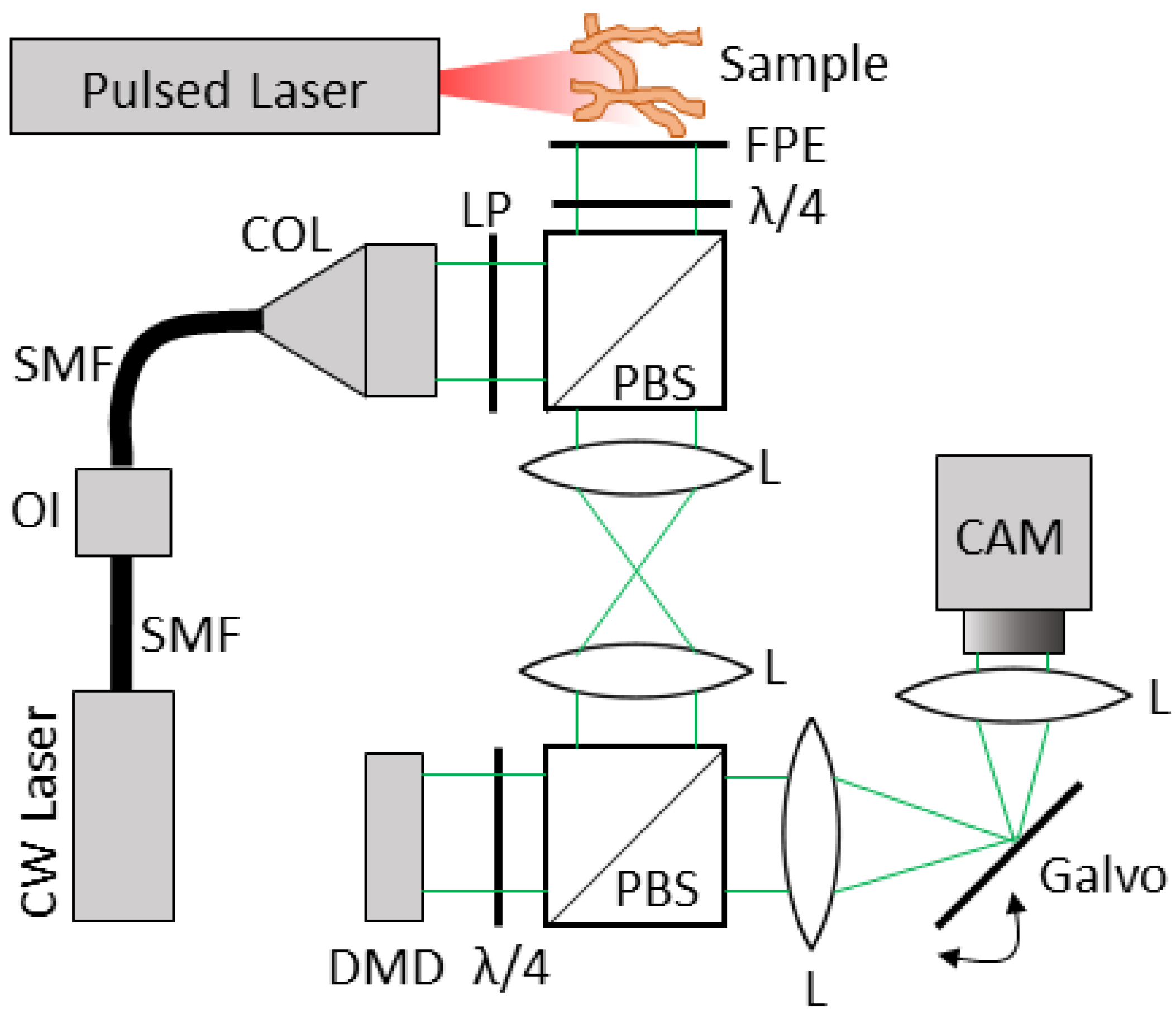
2.1. Optical Setup
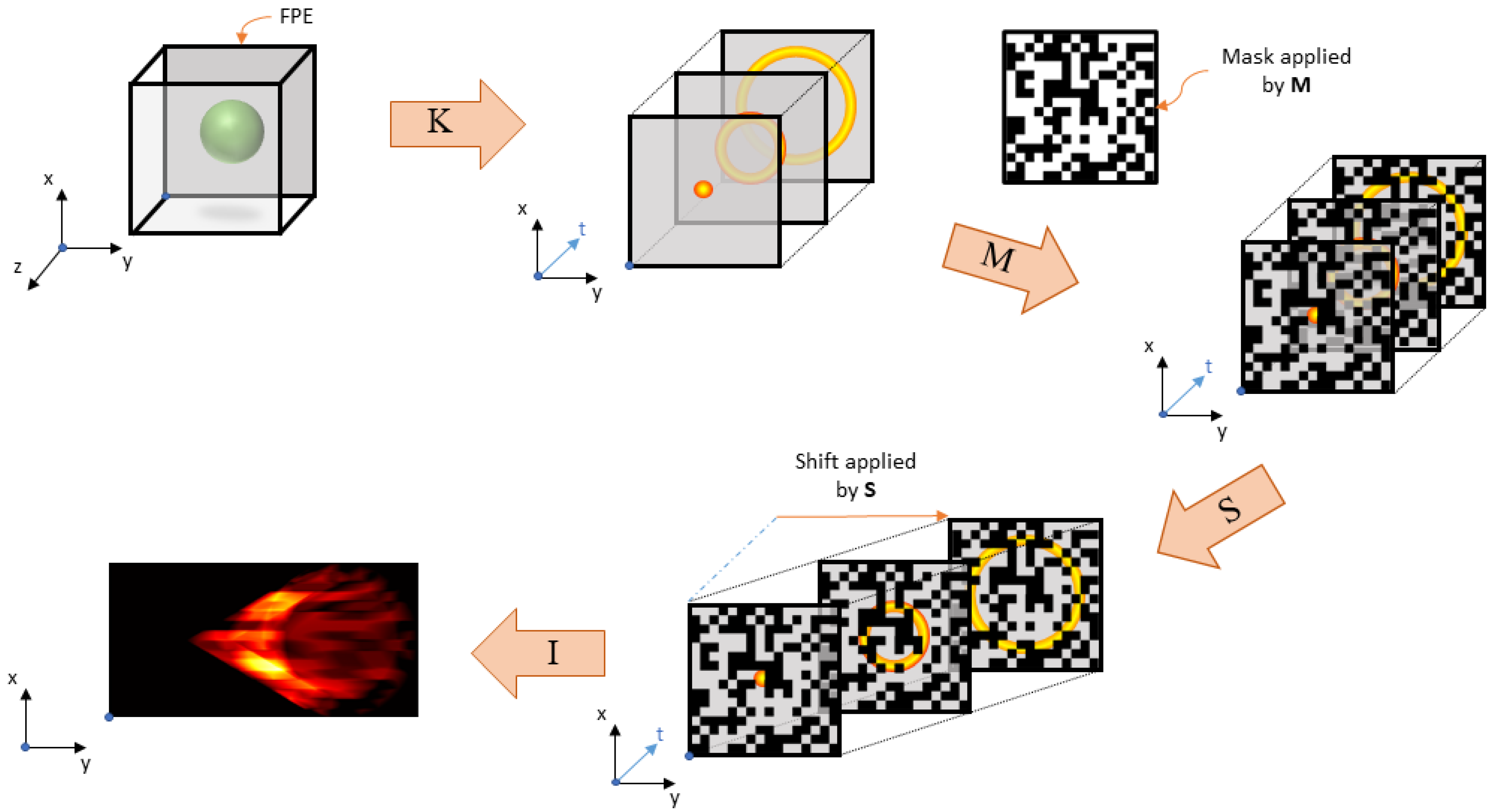
2.2. Continuous Model
2.3. Discrete Model
2.4. Image Reconstruction via Compressed Sensing
2.5. Simulation Setup and Analysis
3. Results
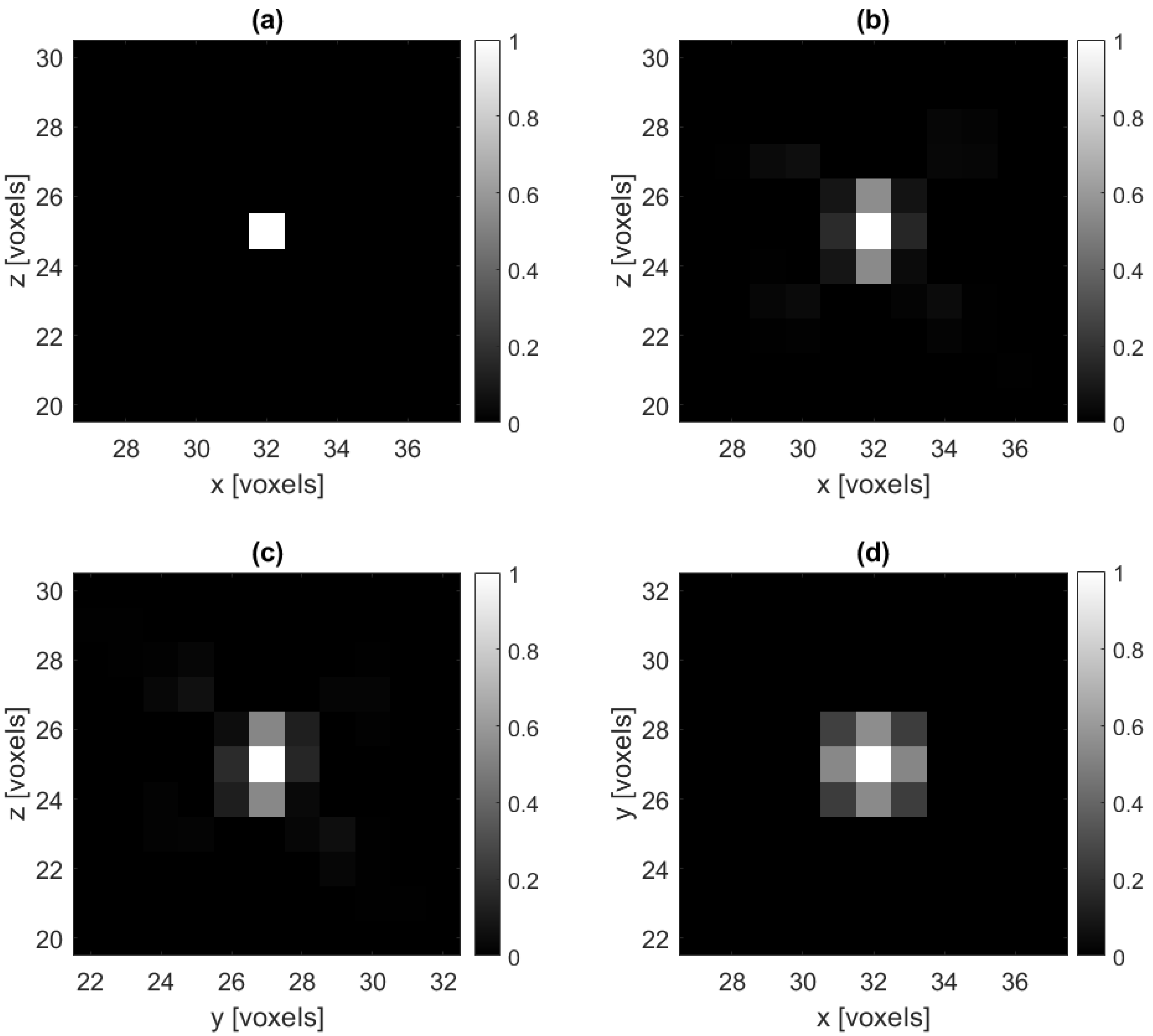
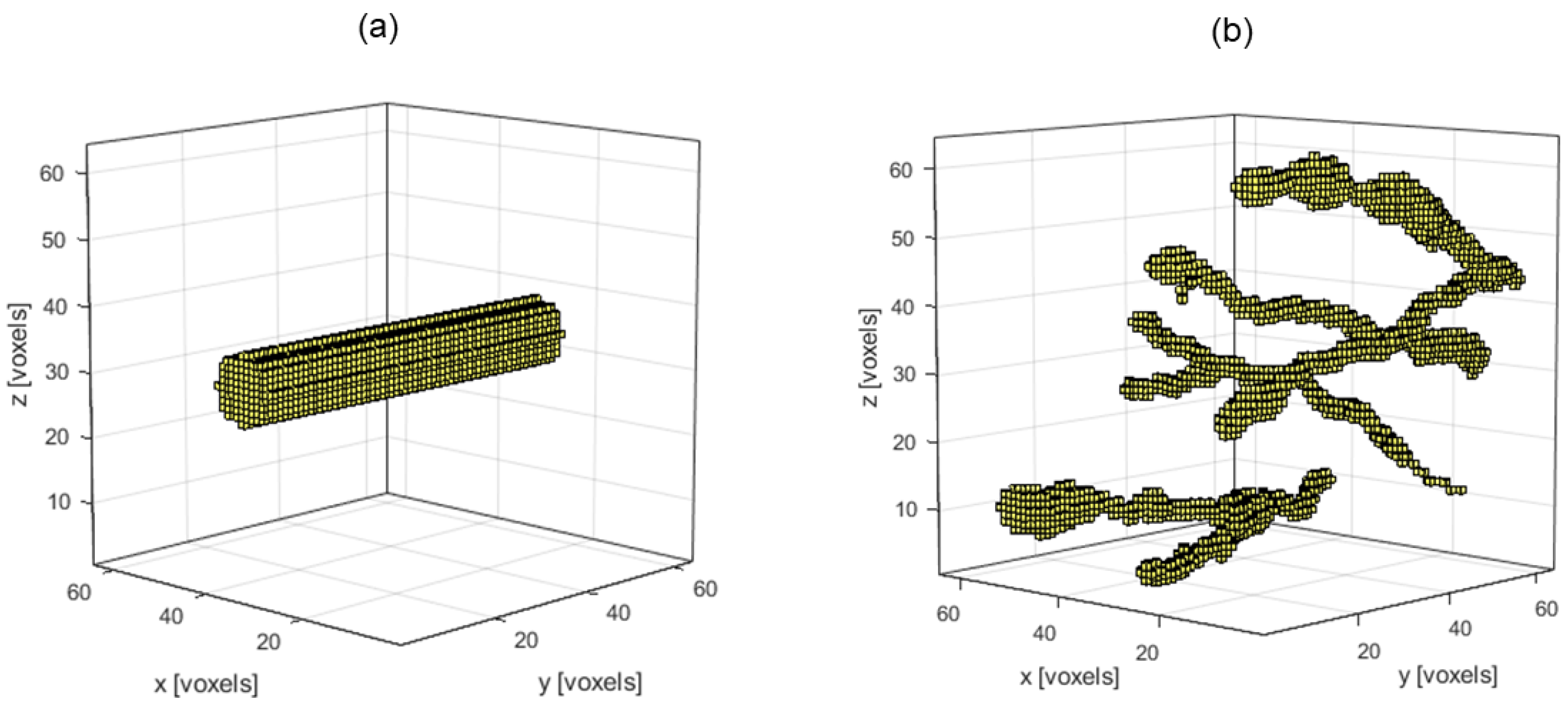
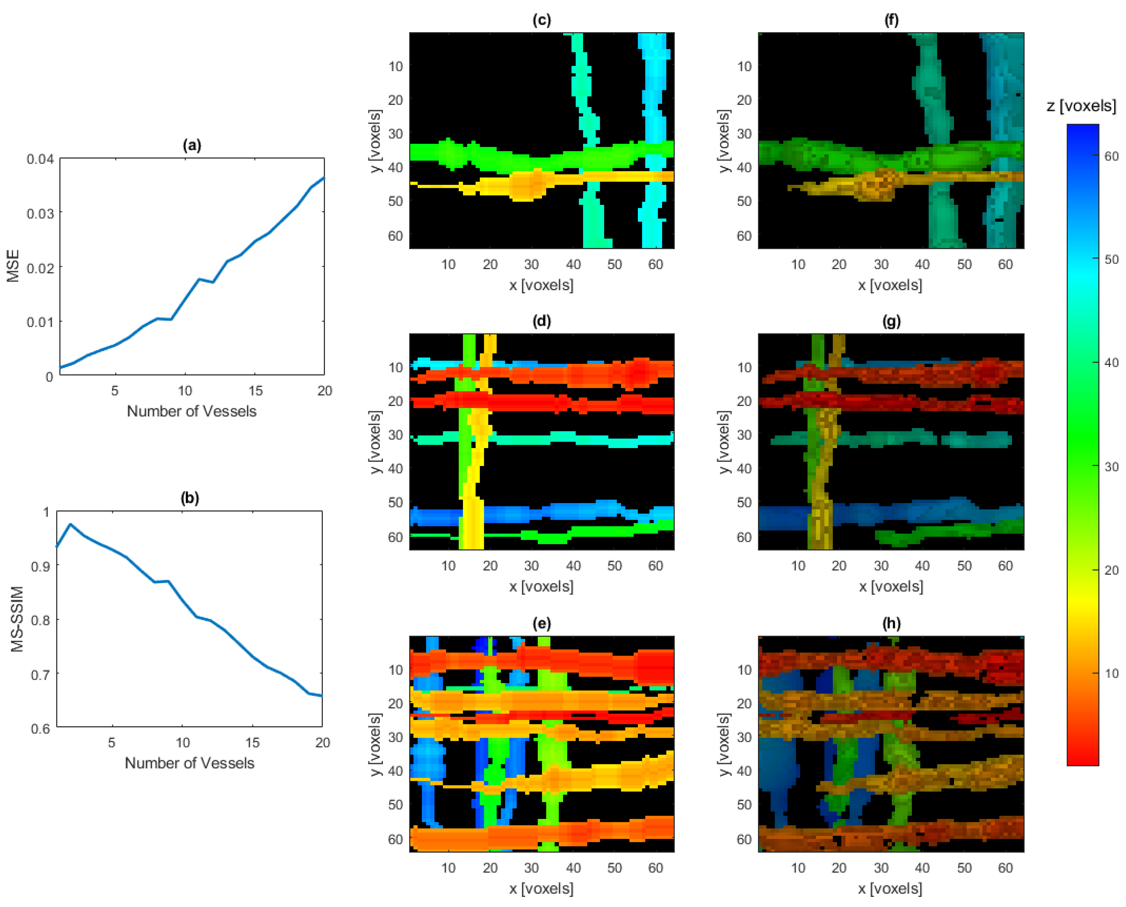
3.1. Baseline Test
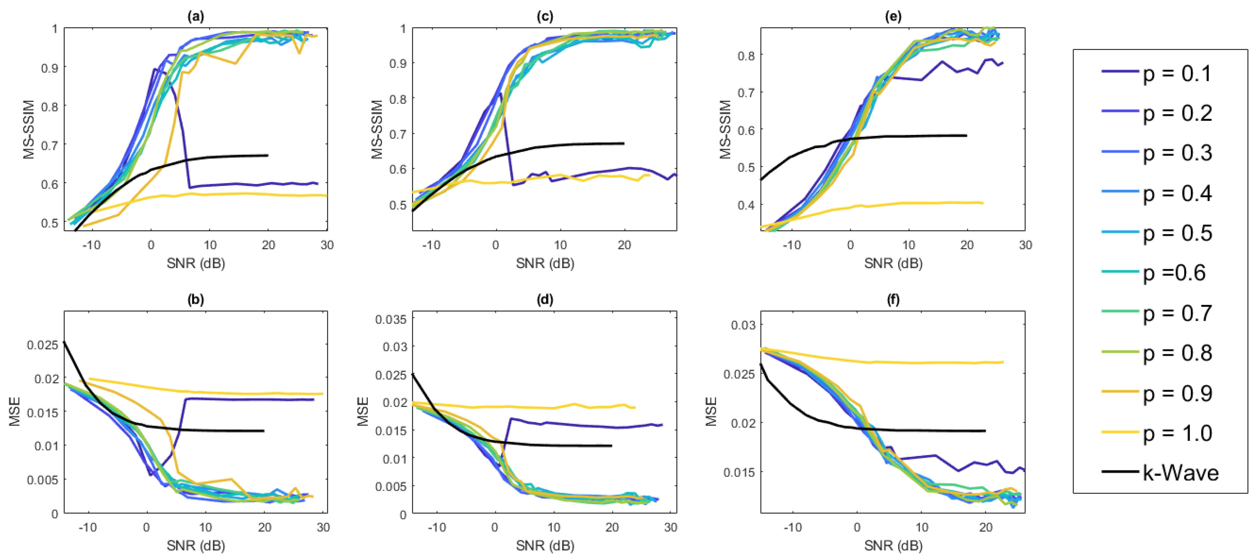
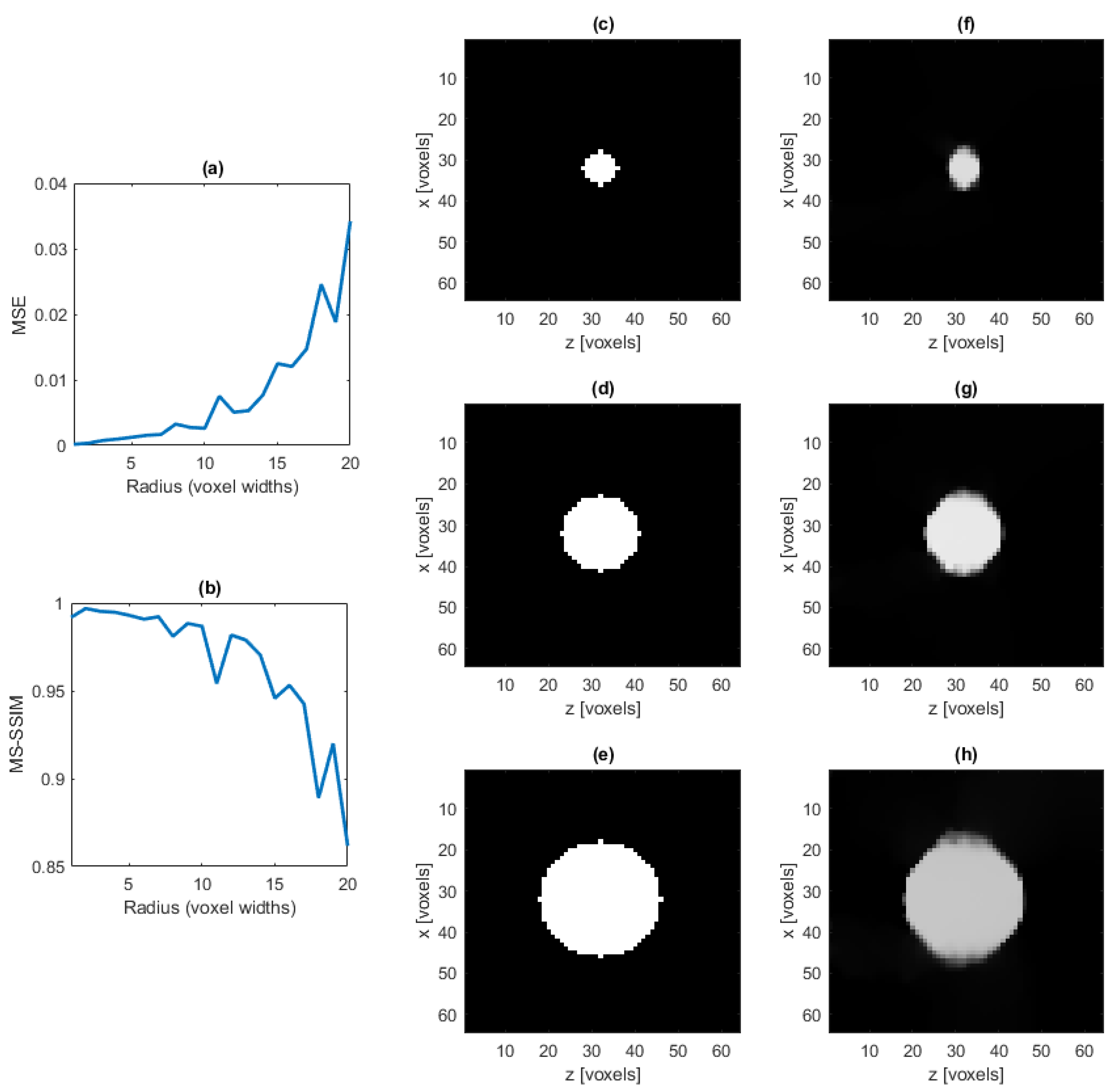
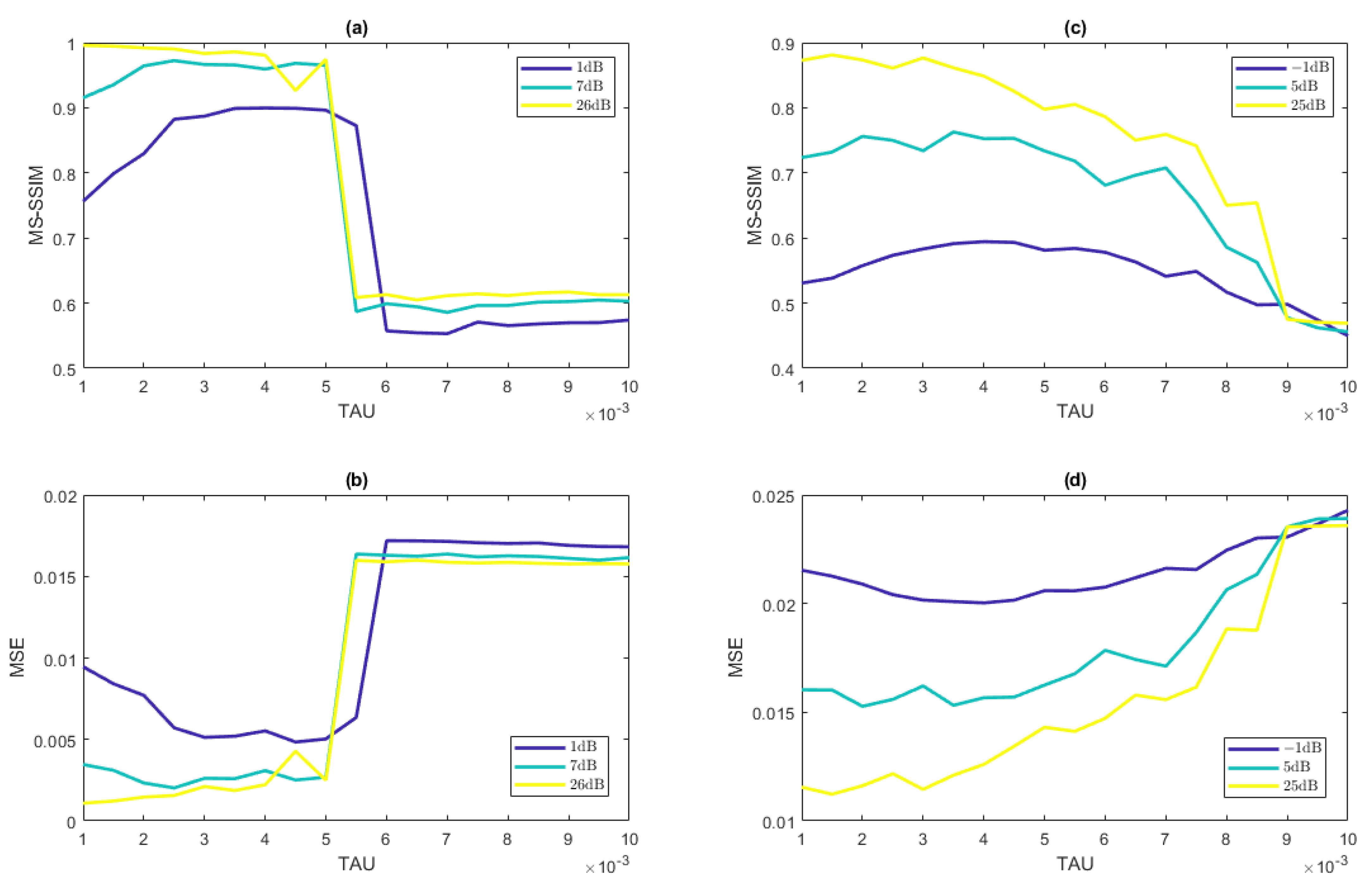
3.2. Simulated Experiments
4. Discussion
Author Contributions
Funding
Data Availability Statement
Acknowledgments
Conflicts of Interest
Abbreviations
| PA | photoacoustic |
| FPE | Fabry–Pérot etalon |
| DMD | digital micro-mirror device |
| IPD | initial pressure distribution |
| TwIST | Two-Step Iterative Shrinkage/Thresholding |
| IST | iterative shrinkage/thresholding |
| IRS | iterative reweighted shrinkage |
| MSE | mean square error |
| MS-SSIM | multi-scale structural similarity |
| SNR | signal-to-noise ratio |
References
- Xu, M.; Wang, L.V. Photoacoustic imaging in biomedicine. Rev. Sci. Instrum. 2006, 77, 041101. [Google Scholar] [CrossRef] [Green Version]
- Mallidi, S.; Luke, G.P.; Emelianov, S. Photoacoustic imaging in cancer detection, diagnosis, and treatment guidance. Trends Biotechnol. 2011, 29, 213–221. [Google Scholar] [CrossRef] [Green Version]
- Wang, X.; Pang, Y.; Ku, G.; Xie, X.; Stoica, G.; Wang, L.V. Noninvasive laser-induced photoacoustic tomography for structural and functional in vivo imaging of the brain. Nat. Biotechnol. 2003, 21, 803–806. [Google Scholar] [CrossRef]
- Wang, L.V.; Hu, S. Photoacoustic tomography: In vivo imaging from organelles to organs. Science 2012, 335, 1458–1462. [Google Scholar] [CrossRef] [Green Version]
- Cox, B.T.; Laufer, J.G.; Beard, P.C.; Arridge, S.R. Quantitative spectroscopic photoacoustic imaging: A review. J. Biomed. Opt. 2012, 17, 061202. [Google Scholar] [CrossRef] [PubMed] [Green Version]
- Wang, L.V.; Yao, J. A practical guide to photoacoustic tomography in the life sciences. Nat. Methods 2016, 13, 627–638. [Google Scholar] [CrossRef]
- Jeon, S.; Kim, J.; Lee, D.; Baik, J.W.; Kim, C. Review on practical photoacoustic microscopy. Photoacoustics 2019, 15, 100141. [Google Scholar] [CrossRef] [PubMed]
- Beard, P.C.; Perennes, F.; Mills, T.N. Transduction mechanisms of the Fabry-Perot polymer film sensing concept for wideband ultrasound detection. IEEE Trans. Ultrason. Ferroelectr. Freq. Control 1999, 46, 1575–1582. [Google Scholar] [CrossRef] [PubMed]
- Zhang, E.; Laufer, J.; Beard, P. Backward-mode multiwavelength photoacoustic scanner using a planar Fabry-Perot polymer film ultrasound sensor for high-resolution three-dimensional imaging of biological tissues. Appl. Opt. 2008, 47, 561–577. [Google Scholar] [CrossRef] [PubMed]
- Huynh, N.; Zhang, E.; Betcke, M.; Arridge, S.; Beard, P.; Cox, B. Single-pixel optical camera for video rate ultrasonic imaging. Optica 2016, 3, 26–29. [Google Scholar] [CrossRef]
- Huynh, N.; Lucka, F.; Zhang, E.Z.; Betcke, M.M.; Arridge, S.R.; Beard, P.C.; Cox, B.T. Single-pixel camera photoacoustic tomography. J. Biomed. Opt. 2019, 24, 121907. [Google Scholar] [CrossRef] [PubMed]
- Li, Y.; Li, L.; Zhu, L.; Maslov, K.; Shi, J.; Hu, P.; Bo, E.; Yao, J.; Liang, J.; Wang, L. Snapshot photoacoustic topography through an ergodic relay for high-throughput imaging of optical absorption. Nat. Photonics 2020, 14, 164–170. [Google Scholar] [CrossRef] [PubMed]
- Qi, D.; Zhang, S.; Yang, C.; He, Y.; Cao, F.; Yao, J.; Ding, P.; Gao, L.; Jia, T.; Liang, J.; et al. Single-shot compressed ultrafast photography: A review. Adv. Photonics 2020, 2, 014003. [Google Scholar] [CrossRef] [Green Version]
- Gao, L.; Liang, J.; Li, C.; Wang, L.V. Single-shot compressed ultrafast photography at one hundred billion frames per second. Nature 2014, 516, 74–77. [Google Scholar] [CrossRef]
- Wang, P.; Liang, J.; Wang, L.V. Single-shot ultrafast imaging attaining 70 trillion frames per second. Nat. Commun. 2020, 11, 1–9. [Google Scholar] [CrossRef]
- Liu, X.; Liu, J.; Jiang, C.; Vetrone, F.; Liang, J. Single-shot compressed optical-streaking ultra-high-speed photography. Opt. Lett. 2019, 44, 1387–1390. [Google Scholar] [CrossRef] [Green Version]
- Pierce, A.D. Acoustics: An Introduction to Its Physical Principles and Applications, 3rd ed.; Springer: Berlin/Heidelberg, Germany, 2019. [Google Scholar]
- Treeby, B.E.; Cox, B.T. k-Wave: MATLAB toolbox for the simulation and reconstruction of photoacoustic wave fields. J. Biomed. Opt. 2010, 15, 021314. [Google Scholar] [CrossRef]
- Candès, E.J.; Romberg, J.; Tao, T. Robust uncertainty principles: Exact signal reconstruction from highly incomplete frequency information. IEEE Trans. Inf. Theory 2006, 52, 489–509. [Google Scholar] [CrossRef] [Green Version]
- Donoho, D.L. Compressed sensing. IEEE Trans. Inf. Theory 2006, 52, 1289–1306. [Google Scholar] [CrossRef]
- Guo, Z.; Li, C.; Song, L.; Wang, L.V. Compressed sensing in photoacoustic tomography in vivo. J. Biomed. Opt. 2010, 15, 021311. [Google Scholar] [CrossRef] [PubMed]
- Arridge, S.; Beard, P.; Betcke, M.; Cox, B.; Huynh, N.; Lucka, F.; Ogunlade, O.; Zhang, E. Accelerated high-resolution photoacoustic tomography via compressed sensing. Phys. Med. Biol. 2016, 61, 8908–8940. [Google Scholar] [CrossRef] [PubMed]
- Haltmeier, M.; Sandbichler, M.; Berer, T.; Bauer-Marschallinger, J.; Burgholzer, P.; Nguyen, L. A sparsification and reconstruction strategy for compressed sensing photoacoustic tomography. J. Acoust. Soc. Am. 2018, 143, 3838–3848. [Google Scholar] [CrossRef]
- Betcke, M.M.; Cox, B.T.; Huynh, N.; Zhang, E.Z.; Beard, P.C.; Arridge, S.R. Acoustic wave field reconstruction from compressed measurements with application in photoacoustic tomography. IEEE Trans. Comput. Imaging 2017, 3, 710–721. [Google Scholar] [CrossRef] [Green Version]
- Kutyniok, G. Theory and applications of compressed sensing. GAMM-Mitteilungen 2013, 36, 79–101. [Google Scholar] [CrossRef] [Green Version]
- Draganic, A.; Orovic, I.; Stankovic, S. On some common compressive sensing recovery algorithms and applications-Review paper. arXiv 2017, arXiv:1705.05216. [Google Scholar]
- Bioucas-Dias, J.M.; Figueiredo, M.A. A new TwIST: Two-step iterative shrinkage/thresholding algorithms for image restoration. IEEE Trans. Image Process. 2007, 16, 2992–3004. [Google Scholar] [CrossRef] [PubMed] [Green Version]
- Shang, R.; Archibald, R.; Gelb, A.; Luke, G.P. Sparsity-based photoacoustic image reconstruction with a linear array transducer and direct measurement of the forward model. J. Biomed. Opt. 2018, 24, 031015. [Google Scholar] [CrossRef]
- Wang, Z.; Simoncelli, E.P.; Bovik, A.C. Multiscale structural similarity for image quality assessment. In Proceedings of the the Thrity-Seventh Asilomar Conference on Signals, Systems & Computers, Pacific Grove, CA, USA, 9–12 November 2003; Volume 2, pp. 1398–1402. [Google Scholar]
- Madsen, E.L.; Zagzebski, J.A.; Banjavie, R.A.; Jutila, R.E. Tissue mimicking materials for ultrasound phantoms. Med. Phys. 1978, 5, 391–394. [Google Scholar] [CrossRef]


| Parameter | Description | Value |
|---|---|---|
| N | length of IPD grid [pixels] | 64 |
| length of computational grid [pixels] | 96 | |
| width of boundary condition layer [pixels] | 15 | |
| speed of sound in the medium [m/s] | 1540 | |
| h | pixel width [m] | 122 |
| f | center frequency [MHz] | 5 |
| T | total time steps | 400 |
| time step size [ns] | 24 | |
| [pixels-widths/s] | 12 | |
| s | downsize factor | 4 |
Publisher’s Note: MDPI stays neutral with regard to jurisdictional claims in published maps and institutional affiliations. |
© 2021 by the authors. Licensee MDPI, Basel, Switzerland. This article is an open access article distributed under the terms and conditions of the Creative Commons Attribution (CC BY) license (https://creativecommons.org/licenses/by/4.0/).
Share and Cite
Green, D.; Gelb, A.; Luke, G.P. Sparsity-Based Recovery of Three-Dimensional Photoacoustic Images from Compressed Single-Shot Optical Detection. J. Imaging 2021, 7, 201. https://doi.org/10.3390/jimaging7100201
Green D, Gelb A, Luke GP. Sparsity-Based Recovery of Three-Dimensional Photoacoustic Images from Compressed Single-Shot Optical Detection. Journal of Imaging. 2021; 7(10):201. https://doi.org/10.3390/jimaging7100201
Chicago/Turabian StyleGreen, Dylan, Anne Gelb, and Geoffrey P. Luke. 2021. "Sparsity-Based Recovery of Three-Dimensional Photoacoustic Images from Compressed Single-Shot Optical Detection" Journal of Imaging 7, no. 10: 201. https://doi.org/10.3390/jimaging7100201
APA StyleGreen, D., Gelb, A., & Luke, G. P. (2021). Sparsity-Based Recovery of Three-Dimensional Photoacoustic Images from Compressed Single-Shot Optical Detection. Journal of Imaging, 7(10), 201. https://doi.org/10.3390/jimaging7100201