Full 3D Microwave Breast Imaging Using a Deep-Learning Technique


Abstract
1. Introduction
2. 3D CSI-Deep-Learning Methodology
2.1. Microwave Imaging via Contrast Source Inversion
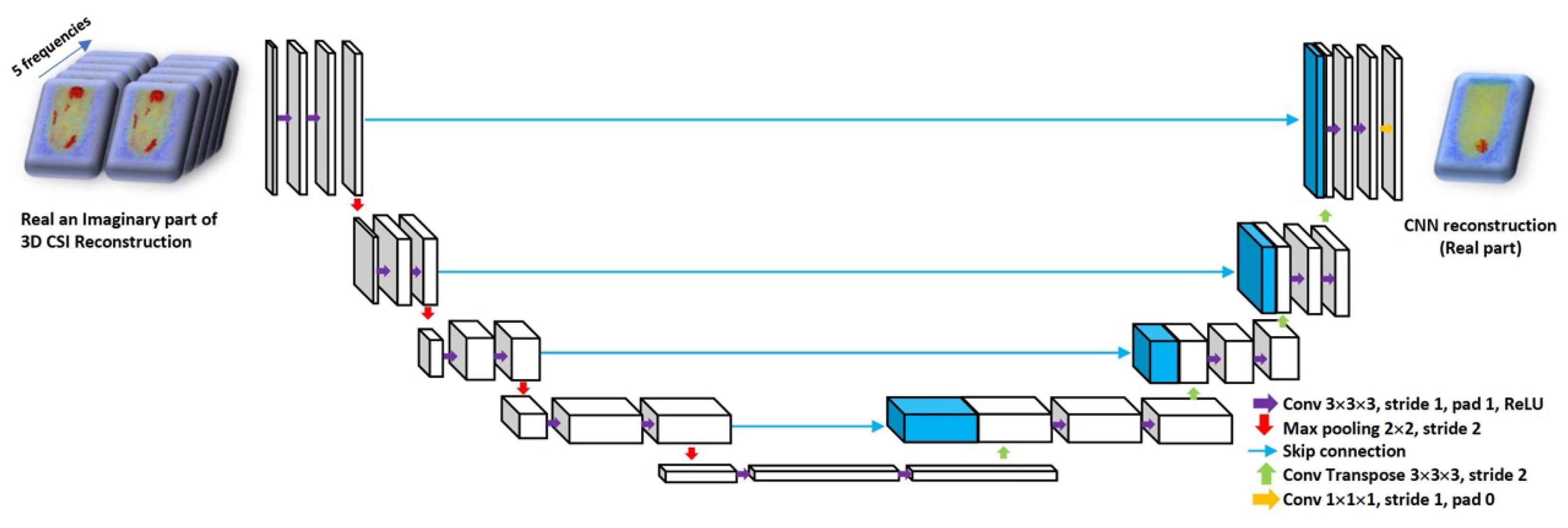
2.2. Machine Learning Approach to Reconstruction
3. Numerical Experiments
3.1. Datasets
3.2. Network Training
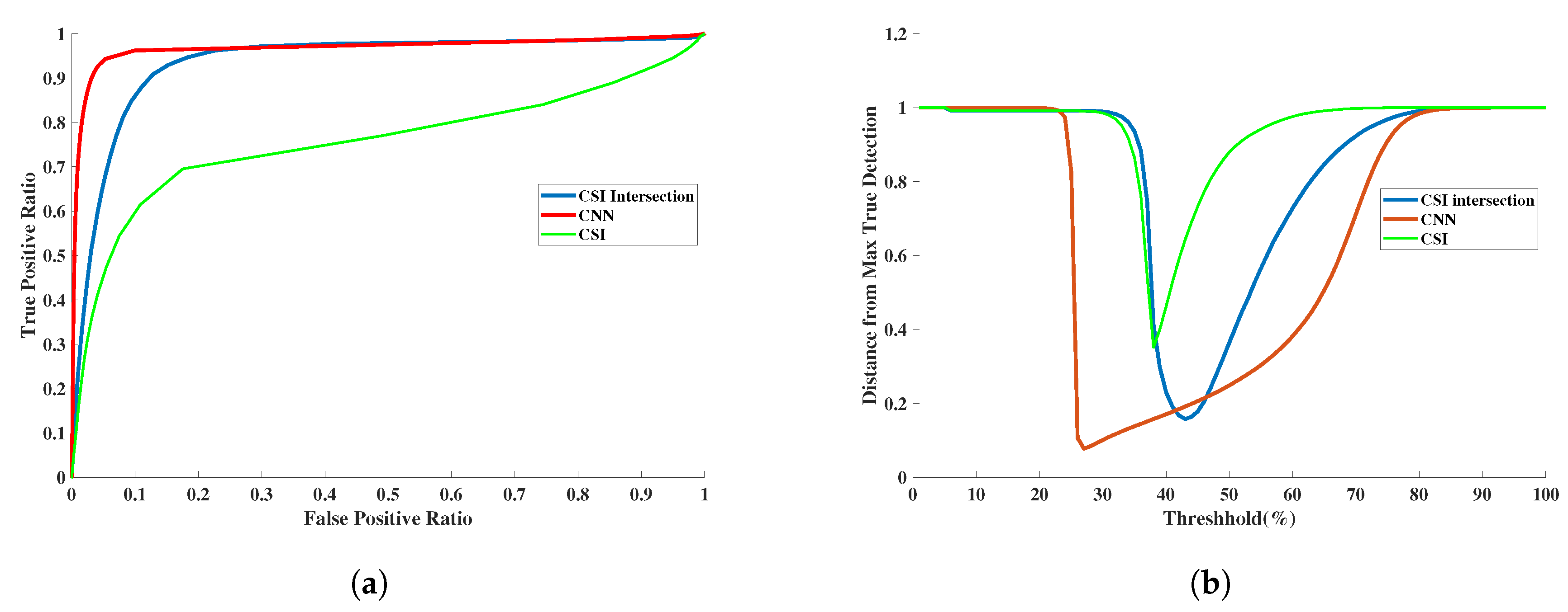
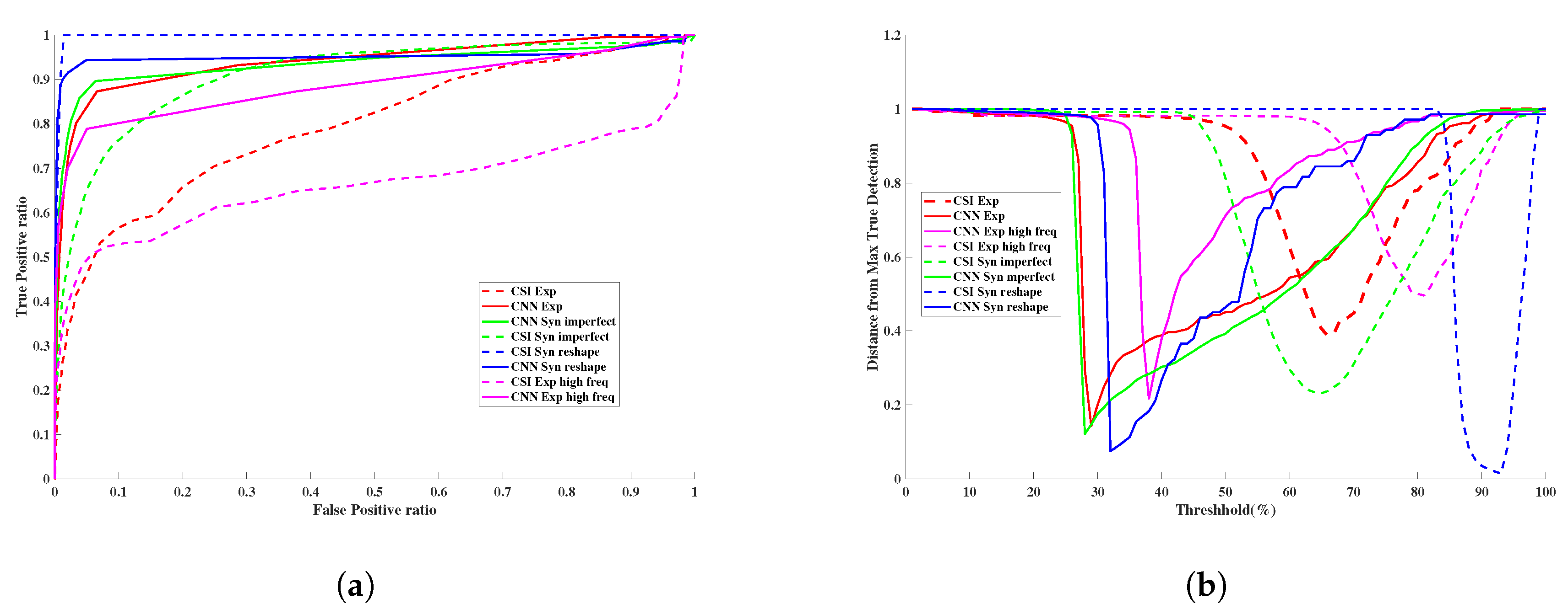
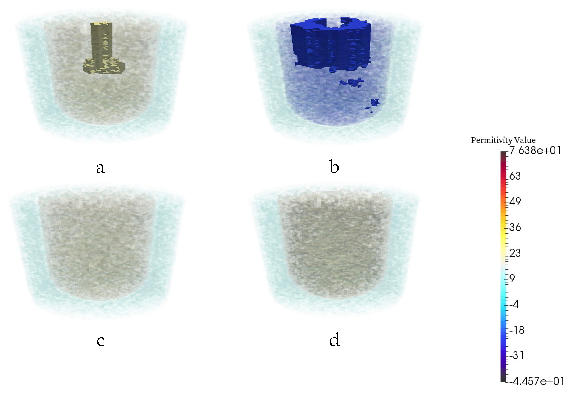
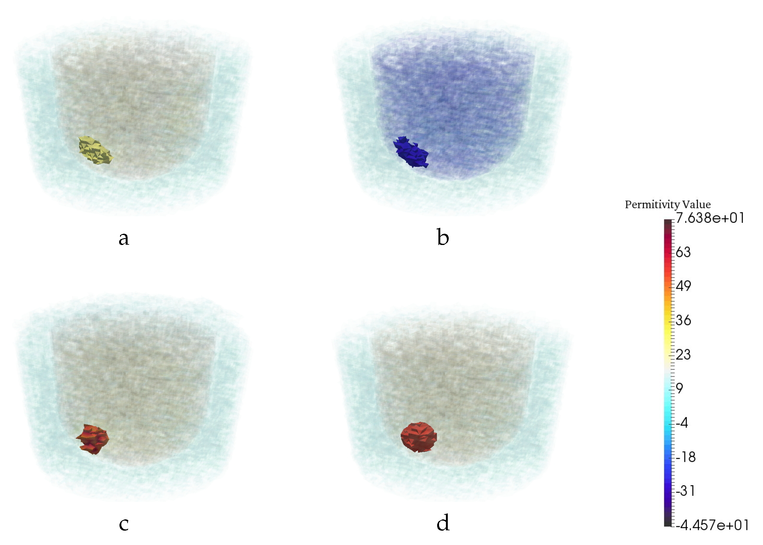
3.3. Quantitative Assessment
3.4. Assessment of Robustness
3.4.1. Robustness to Changes in Frequency
3.4.2. Robustness to Changes in Breast Phantom Geometry
3.4.3. Robustness to Imperfections in Prior Information
3.4.4. Robustness to Breast Phantom with No Tumor
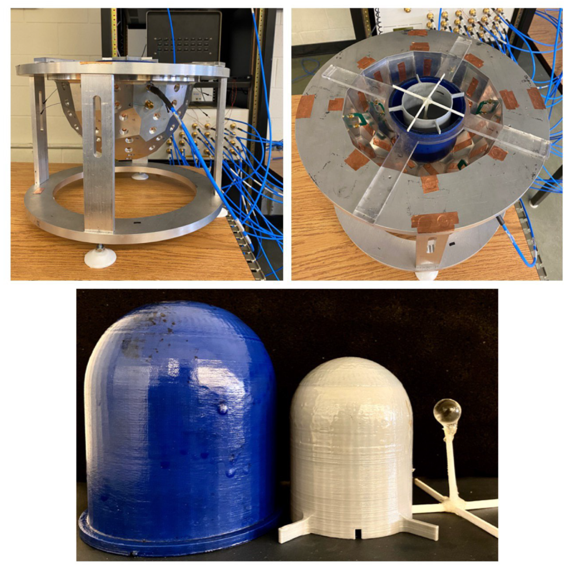
4. Experimental Tests and Results
5. Conclusions
Author Contributions
Funding
Conflicts of Interest
References
- O’Loughlin, D.; O’Halloran, M.J.; Moloney, B.M.; Glavin, M.; Jones, E.; Elahi, M.A. Microwave Breast Imaging: Clinical Advances and Remaining Challenges. IEEE Trans. Biomed. Eng. 2018, 65, 2580–2590. [Google Scholar] [CrossRef]
- Bolomey, J.C. Crossed Viewpoints on Microwave-Based Imaging for Medical Diagnosis: From Genesis to Earliest Clinical Outcomes. In The World of Applied Electromagnetics: In Appreciation of Magdy Fahmy Iskander; Lakhtakia, A., Furse, C.M., Eds.; Springer International Publishing: Cham, Switzerland, 2018; pp. 369–414. [Google Scholar]
- Lazebnik, M.; Popovic, D.; McCartney, L.; Watkins, C.B.; Lindstrom, M.J.; Harter, J.; Sewall, S.; Ogilvie, T.; Magliocco, A.; Breslin, T.M.; et al. A large-scale study of the ultrawideband microwave dielectric properties of normal, benign and malignant breast tissues obtained from cancer surgeries. Phys. Med. Biol. 2007, 52, 6093. [Google Scholar] [CrossRef]
- Halter, R.J.; Zhou, T.; Meaney, P.M.; Hartov, A.; Barth, R.J., Jr.; Rosenkranz, K.M.; Wells, W.A.; Kogel, C.A.; Borsic, A.; Rizzo, E.J.; et al. The correlation of in vivo and ex vivo tissue dielectric properties to validate electromagnetic breast imaging: Initial clinical experience. Physiol. Meas. 2009, 30, S121. [Google Scholar] [CrossRef]
- Pastorino, M. Microwave Imaging; John Wiley & Sons: Hoboken, NJ, USA, 2010. [Google Scholar]
- Van den Berg, P.M.; Kleinman, R.E. A contrast source inversion method. Inverse Probl. 1997, 13, 1607–1620. [Google Scholar] [CrossRef]
- Abubakar, A.; van den Berg, P.M.; Mallorqui, J.J. Imaging of biomedical data using a multiplicative regularized contrast source inversion method. IEEE Trans. Microw. Theory Tech. 2002, 50, 1761–1771. [Google Scholar] [CrossRef]
- Zakaria, A.; Gilmore, C.; LoVetri, J. Finite-element contrast source inversion method for microwave imaging. Inverse Probl. 2010, 26, 115010. [Google Scholar] [CrossRef]
- Kurrant, D.; Baran, A.; LoVetri, J.; Fear, E. Integrating prior information into microwave tomography Part 1: Impact of detail on image quality. Med. Phys. 2017, 44, 6461–6481. [Google Scholar] [CrossRef] [PubMed]
- Baran, A.; Kurrant, D.; Fear, E.; LoVetri, J. Integrating prior information into microwave tomography part 2: Impact of errors in prior information on microwave tomography image quality. Med. Phys. 2017, 44, 6482–6503. [Google Scholar]
- Chen, X. Computational Methods for Electromagnetic Inverse Scattering; Wiley Online Library: Hoboken, NJ, USA, 2018. [Google Scholar]
- Goodfellow, I.; Bengio, Y.; Courville, A. Deep Learning; MIT Press: Cambridge, MA, USA, 2016; Available online: http://www.deeplearningbook.org (accessed on 10 August 2020).
- Ronneberger, O.; Fischer, P.; Brox, T. U-Net: Convolutional Networks for Biomedical Image Segmentation. arXiv 2015, arXiv:1505.04597. [Google Scholar]
- Wang, G.; Li, W.; Zuluaga, M.A.; Pratt, R.; Patel, P.A.; Aertsen, M.; Doel, T.; David, A.L.; Deprest, J.; Ourselin, S.; et al. Interactive Medical Image Segmentation Using Deep Learning With Image-Specific Fine Tuning. IEEE Trans. Med. Imaging 2018, 37, 1562–1573. [Google Scholar] [CrossRef]
- Shin, H.; Roth, H.R.; Gao, M.; Lu, L.; Xu, Z.; Nogues, I.; Yao, J.; Mollura, D.; Summers, R.M. Deep Convolutional Neural Networks for Computer-Aided Detection: CNN Architectures, Dataset Characteristics and Transfer Learning. IEEE Trans. Med Imaging 2016, 35, 1285–1298. [Google Scholar] [CrossRef]
- McCann, M.T.; Jin, K.H.; Unser, M. Convolutional Neural Networks for Inverse Problems in Imaging: A Review. IEEE Signal Process. Mag. 2017, 34, 85–95. [Google Scholar] [CrossRef]
- Xie, Y.; Xia, Y.; Zhang, J.; Song, Y.; Feng, D.; Fulham, M.; Cai, W. Knowledge-based Collaborative Deep Learning for Benign-Malignant Lung Nodule Classification on Chest CT. IEEE Trans. Med. Imaging 2019, 38, 991–1004. [Google Scholar] [CrossRef] [PubMed]
- Kang, E.; Min, J.; Ye, J.C. A deep convolutional neural network using directional wavelets for low-dose X-ray CT reconstruction. Med. Phys. 2017, 44, e360–e375. [Google Scholar] [CrossRef] [PubMed]
- Han, Y.; Yoo, J.J.; Ye, J.C. Deep Residual Learning for Compressed Sensing CT Reconstruction via Persistent Homology Analysis. arXiv 2016, arXiv:1611.06391. [Google Scholar]
- Jin, K.H.; McCann, M.T.; Froustey, E.; Unser, M. Deep Convolutional Neural Network for Inverse Problems in Imaging. IEEE Trans. Image Process. 2017, 26, 4509–4522. [Google Scholar] [CrossRef]
- Han, Y.; Yoo, J.; Kim, H.H.; Shin, H.J.; Sung, K.; Ye, J.C. Deep learning with domain adaptation for accelerated projection-reconstruction MR. Magn. Reson. Med. 2018, 80, 1189–1205. [Google Scholar] [CrossRef]
- Rahama, Y.A.; Aryani, O.A.; Din, U.A.; Awar, M.A.; Zakaria, A.; Qaddoumi, N. Novel Microwave Tomography System Using a Phased-Array Antenna. IEEE Trans. Microw. Theory Tech. 2018, 66, 5119–5128. [Google Scholar] [CrossRef]
- Rekanos, I.T. Neural-network-based inverse-scattering technique for online microwave medical imaging. IEEE Trans. Magn. 2002, 38, 1061–1064. [Google Scholar] [CrossRef]
- Li, L.; Wang, L.G.; Teixeira, F.L.; Liu, C.; Nehorai, A.; Cui, T.J. DeepNIS: Deep Neural Network for Nonlinear Electromagnetic Inverse Scattering. IEEE Trans. Antennas Propag. 2019, 67, 1819–1825. [Google Scholar] [CrossRef]
- Khoshdel, V.; Ashraf, A.L.J. Enhancement of Multimodal Microwave-Ultrasound Breast Imaging Using a Deep-Learning Technique. Sensors 2019, 19, 4050. [Google Scholar] [CrossRef] [PubMed]
- Rana, S.P.; Dey, M.; Tiberi, G.; Sani, L.; Vispa, A.; Raspa, G.; Duranti, M.; Ghavami, M.; Dudley, S. Machine learning approaches for automated lesion detection in microwave breast imaging clinical data. Sci. Rep. 2019, 9, 1–12. [Google Scholar] [CrossRef] [PubMed]
- Asefi, M.; Baran, A.; LoVetri, J. An Experimental Phantom Study for Air-Based Quasi-Resonant Microwave Breast Imaging. IEEE Trans. Microw. Theory Tech. 2019, 67, 3946–3954. [Google Scholar] [CrossRef]
- Meaney, P.M.; Paulsen, K.D.; Geimer, S.D.; Haider, S.A.; Fanning, M.W. Quantification of 3-D field effects during 2-D microwave imaging. IEEE Trans. Biomed. Eng. 2002, 49, 708–720. [Google Scholar] [CrossRef]
- Golnabi, A.H.; Meaney, P.M.; Epstein, N.R.; Paulsen, K.D. Microwave imaging for breast cancer detection: Advances in three–dimensional image reconstruction. In Proceedings of the 2011 Annual International Conference of the IEEE Engineering in Medicine and Biology Society, Boston, MA, USA, 30 August–3 September 2011; pp. 5730–5733. [Google Scholar]
- Golnabi, A.H.; Meaney, P.M.; Geimer, S.D.; Paulsen, K.D. 3-D Microwave Tomography Using the Soft Prior Regularization Technique: Evaluation in Anatomically Realistic MRI-Derived Numerical Breast Phantoms. IEEE Trans. Biomed. Eng. 2019, 66, 2566–2575. [Google Scholar] [CrossRef]
- Abdollahi, N.; Kurrant, D.; Mojabi, P.; Omer, M.; Fear, E.; LoVetri, J. Incorporation of Ultrasonic Prior Information for Improving Quantitative Microwave Imaging of Breast. IEEE J. Multiscale Multiphys. Comput. Tech. 2019, 4, 98–110. [Google Scholar] [CrossRef]
- Gil Cano, J.D.; Fasoula, A.D.L.; Bernard, J.G. Wavelia Breast Imaging: The Optical Breast Contour Detection Subsystem. Appl. Sci. 2020, 10, 1234. [Google Scholar] [CrossRef]
- Odle, T.G. Breast imaging artifacts. Radiol. Technol. 2015, 89, 428. [Google Scholar]
- Chew, W.C.; Wang, Y.M. Reconstruction of two-dimensional permittivity distribution using the distorted Born iterative method. IEEE Trans. Med. Imaging 1990, 9, 218–225. [Google Scholar] [CrossRef]
- Joachimowicz, N.; Pichot, C.; Hugonin, J.P. Inverse scattering: An iterative numerical method for electromagnetic imaging. IEEE Trans. Antennas Propag. 1991, 39, 1742–1753. [Google Scholar] [CrossRef]
- Franchois, A.; Pichot, C. Microwave imaging-complex permittivity reconstruction with a Levenberg-Marquardt method. IEEE Trans. Antennas Propag. 1997, 45, 203–215. [Google Scholar] [CrossRef]
- Bulyshev, A.; Semenov, S.; Souvorov, A.; Svenson, R.; Nazarov, A.; Sizov, Y.; Tatsis, G. Computational modeling of three-dimensional microwave tomography of breast cancer. IEEE Trans. Biomed. Eng. 2001, 48, 1053–1056. [Google Scholar] [CrossRef] [PubMed]
- Meaney, P.M.; Geimer, S.D.; Paulsen, K.D. Two-step inversion with a logarithmic transformation for microwave breast imaging. Med. Phys. 2017, 44, 4239–4251. [Google Scholar] [CrossRef]
- Mojabi, P.; LoVetri, J. Overview and classification of some regularization techniques for the Gauss-Newton inversion method applied to inverse scattering problems. IEEE Trans. Antennas Propag. 2009, 57, 2658–2665. [Google Scholar] [CrossRef]
- Van den Berg, P.; Abubakar, A.; Fokkema, J. Multiplicative regularization for contrast profile inversion. Radio Sci. 2003, 38. [Google Scholar] [CrossRef]
- Zakaria, A.; Jeffrey, I.; LoVetri, J.; Zakaria, A. Full-Vectorial Parallel Finite-Element Contrast Source Inversion Method. Prog. Electromagn. Res. 2013, 142, 463–483. [Google Scholar] [CrossRef]
- Nemez, K.; Baran, A.; Asefi, M.; LoVetri, J. Modeling Error and Calibration Techniques for a Faceted Metallic Chamber for Magnetic Field Microwave Imaging. IEEE Trans. Microw. Theory Techn. 2017, 65, 4347–4356. [Google Scholar] [CrossRef]
- He, K.; Zhang, X.; Ren, S.; Sun, J. Deep Residual Learning for Image Recognition. In Proceedings of the 2016 IEEE Conference on Computer Vision and Pattern Recognition (CVPR), Las Vegas, NV, USA, 27–30 June 2016; pp. 770–778. [Google Scholar]
- Trabelsi, C.; Bilaniuk, O.; Zhang, Y.; Serdyuk, D.; Subramanian, S.; Santos, J.F.; Mehri, S.; Rostamzadeh, N.; Bengio, Y.; Pal, C. Deep Complex Networks. arXiv 2018, arXiv:1705.09792. [Google Scholar]
- Krizhevsky, A.; Sutskever, I.; Hinton, G.E. ImageNet Classification with Deep Convolutional Neural Networks. In Advances in Neural Information Processing Systems 25; Pereira, F., Burges, C.J.C., Bottou, L., Weinberger, K.Q., Eds.; Curran Associates, Inc.: Red Hook, NY, USA, 2012; pp. 1097–1105. [Google Scholar]
- Glorot, X.; Bengio, Y. Understanding the difficulty of training deep feedforward neural networks. In Proceedings of the International Conference on Artificial Intelligence and Statistics (AISTATS’10), Society for Artificial Intelligence and Statistics, Tübingen, Germany, 21–23 April 2010. [Google Scholar]
- Hanley, J.; McNeil, B. The meaning and use of the area under a receiver operating characteristic (ROC) curve. Radiology 1982, 43, 29–36. [Google Scholar] [CrossRef]


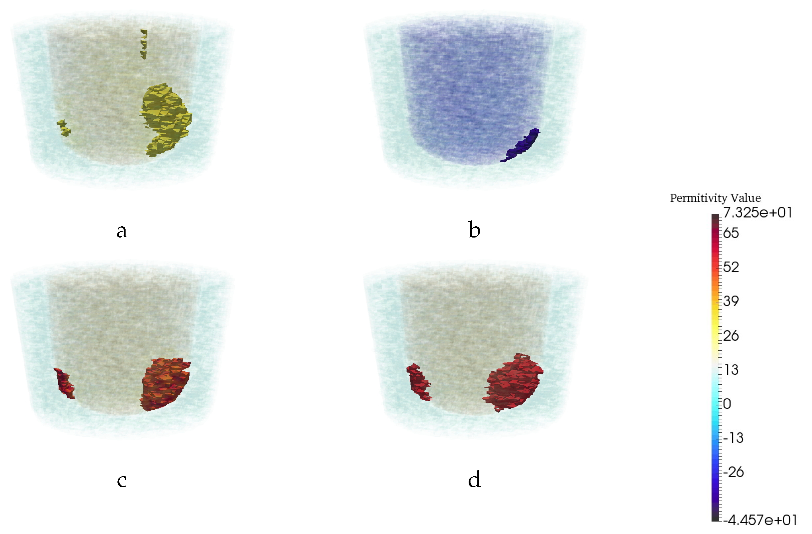
| Permittivity | |||
|---|---|---|---|
| Air | Fat | Fibroglandular | Tumor |
| 1 − 0.001j | 3 − 0.6j | 20 − 21.6j | 56.3 − 30j |
| RMS Error | AUC | |||
|---|---|---|---|---|
| CSI | CNN | CSI | CNN | |
| Synthetic Data | 1.4356 | 1.161 | 0.935 | 0.957 |
| Exprimental Data | 1.250 | 1.172 | 0.794 | 0.938 |
© 2020 by the authors. Licensee MDPI, Basel, Switzerland. This article is an open access article distributed under the terms and conditions of the Creative Commons Attribution (CC BY) license (http://creativecommons.org/licenses/by/4.0/).
Share and Cite
Khoshdel, V.; Asefi, M.; Ashraf, A.; LoVetri, J. Full 3D Microwave Breast Imaging Using a Deep-Learning Technique. J. Imaging 2020, 6, 80. https://doi.org/10.3390/jimaging6080080
Khoshdel V, Asefi M, Ashraf A, LoVetri J. Full 3D Microwave Breast Imaging Using a Deep-Learning Technique. Journal of Imaging. 2020; 6(8):80. https://doi.org/10.3390/jimaging6080080
Chicago/Turabian StyleKhoshdel, Vahab, Mohammad Asefi, Ahmed Ashraf, and Joe LoVetri. 2020. "Full 3D Microwave Breast Imaging Using a Deep-Learning Technique" Journal of Imaging 6, no. 8: 80. https://doi.org/10.3390/jimaging6080080
APA StyleKhoshdel, V., Asefi, M., Ashraf, A., & LoVetri, J. (2020). Full 3D Microwave Breast Imaging Using a Deep-Learning Technique. Journal of Imaging, 6(8), 80. https://doi.org/10.3390/jimaging6080080