Color Photometric Stereo Using Multi-Band Camera Constrained by Median Filter and Occluding Boundary


Abstract
1. Introduction
2. Related Work
3. Multispectral Color Photometric Stereo Method
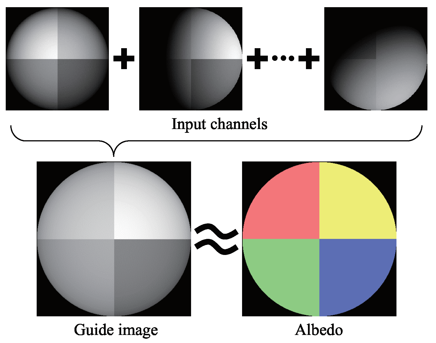
3.1. Image Formulation
3.2. Cost Function
3.3. Determining Surface Normal and Albedo
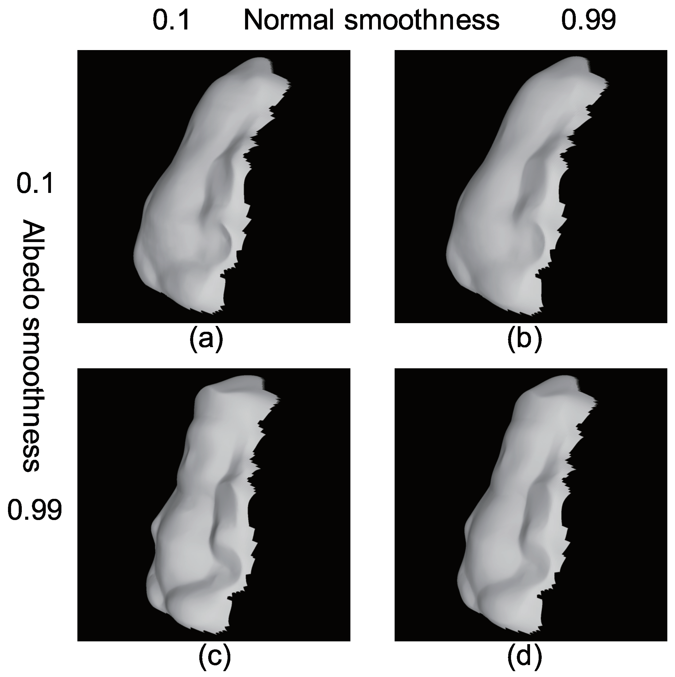
3.4. Smoothness Constraint for Surface Normal
3.5. Smoothness Constraint for Albedo
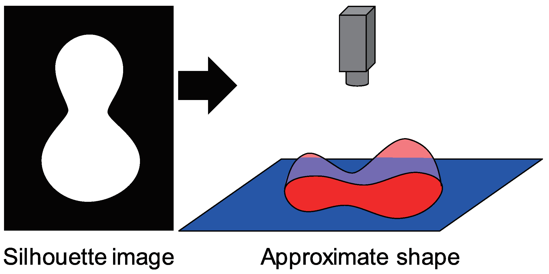
3.6. Occluding Boundary Constraint and Initial Value of Surface Normal
3.7. Initial Value of Albedo
3.8. Update Rule
3.9. Outlier Detection
3.10. Calculating Height from Surface Normal
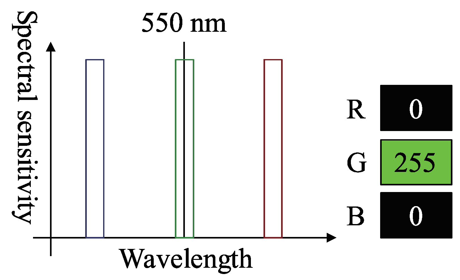
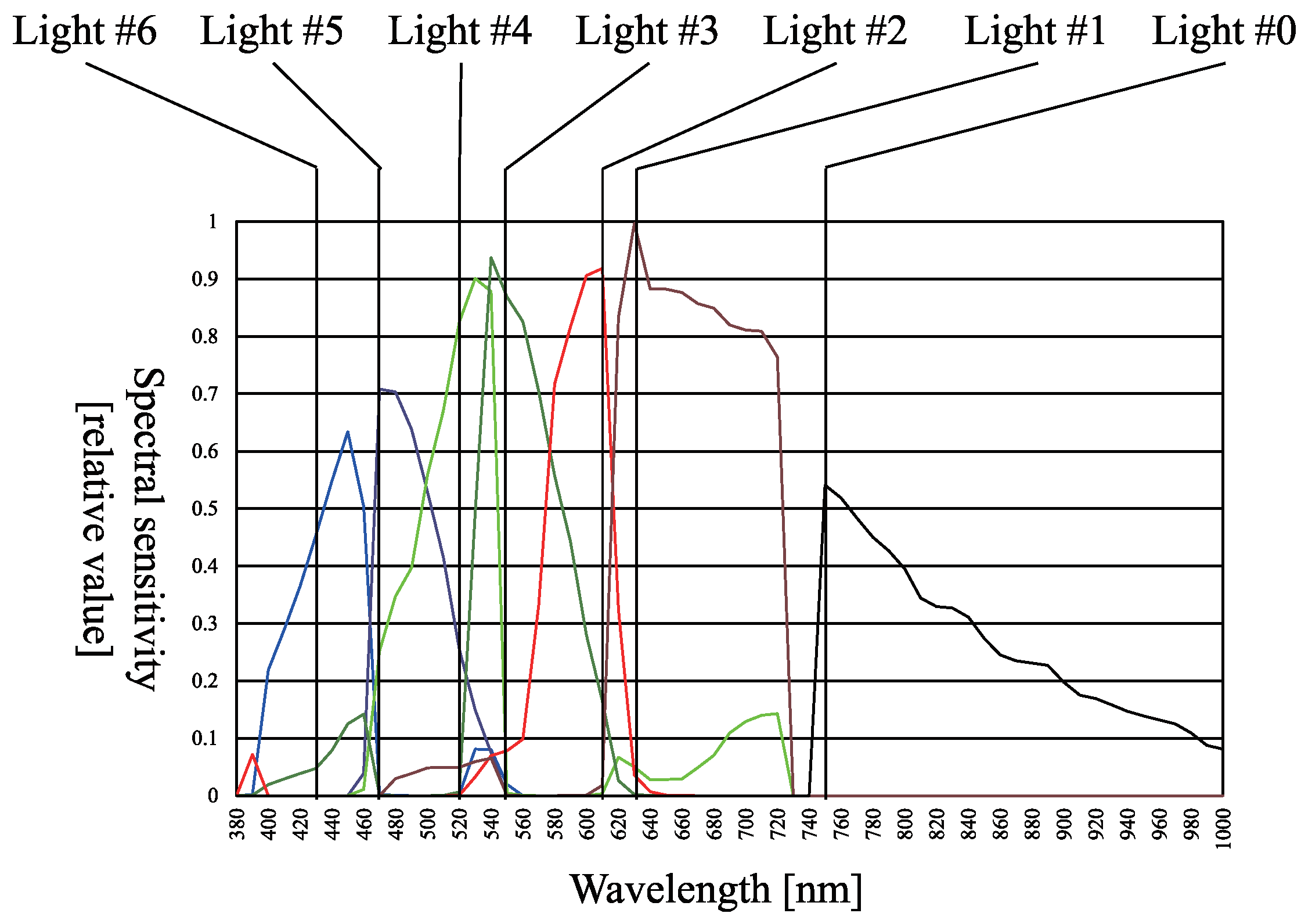
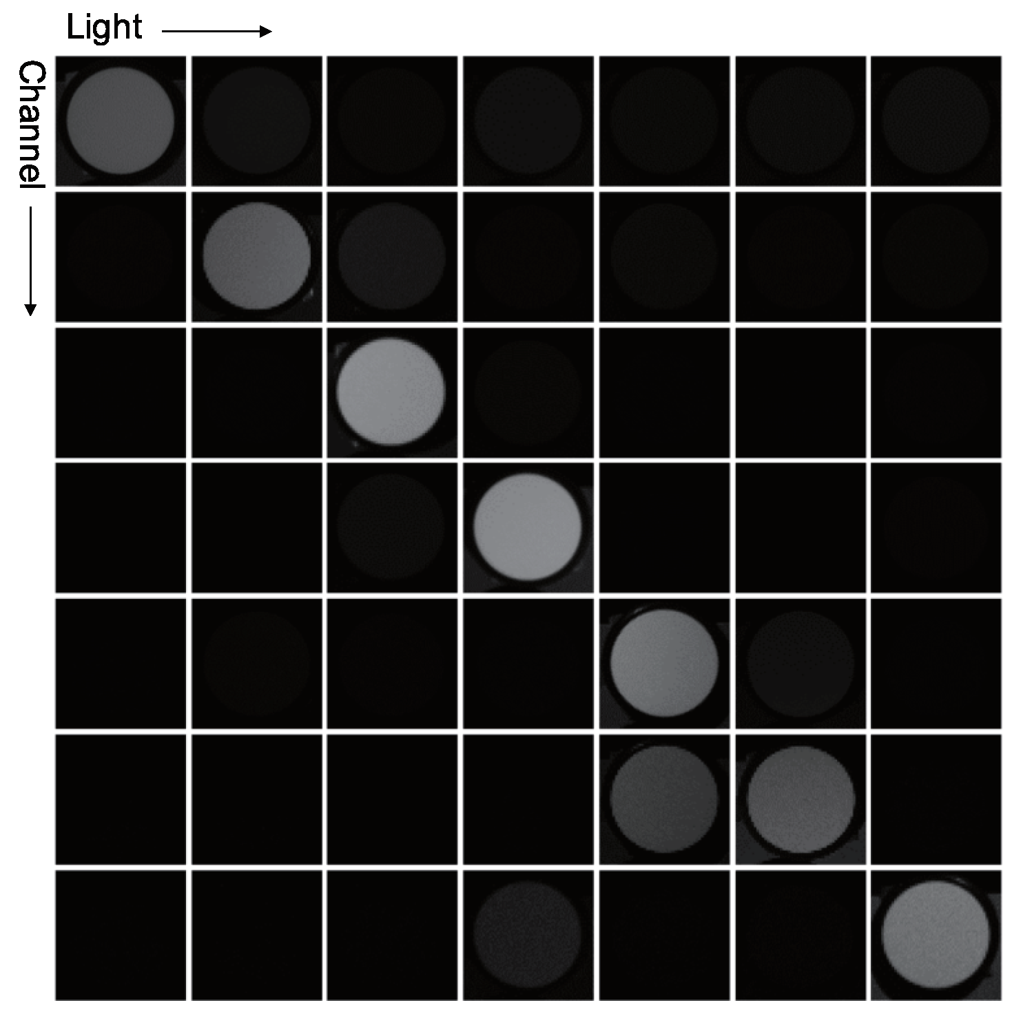
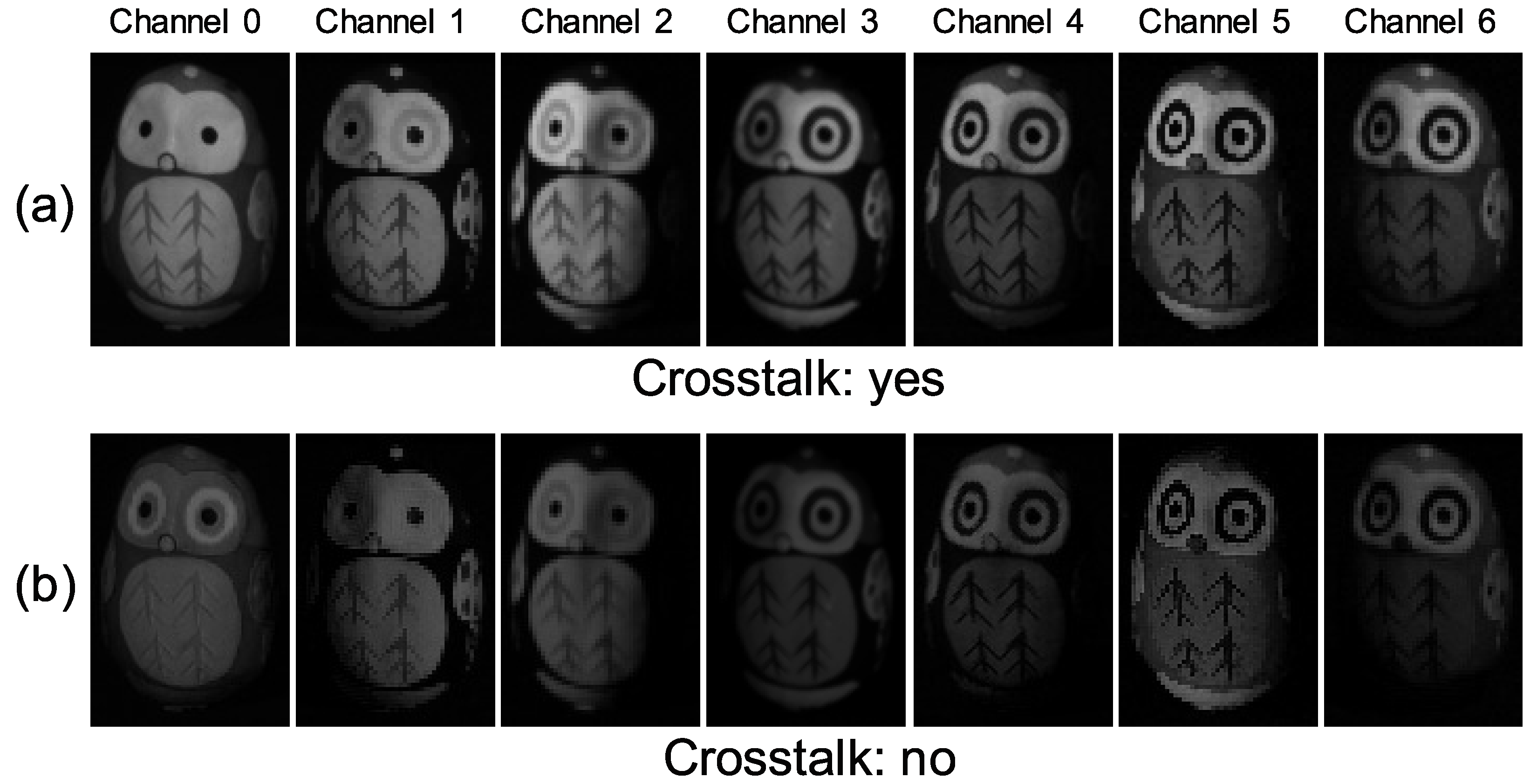
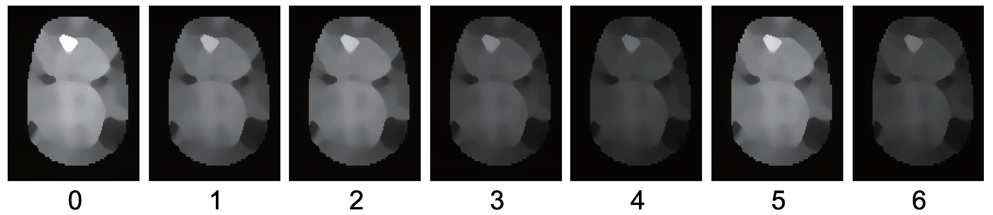
3.11. Channel Crosstalk
4. Experiment
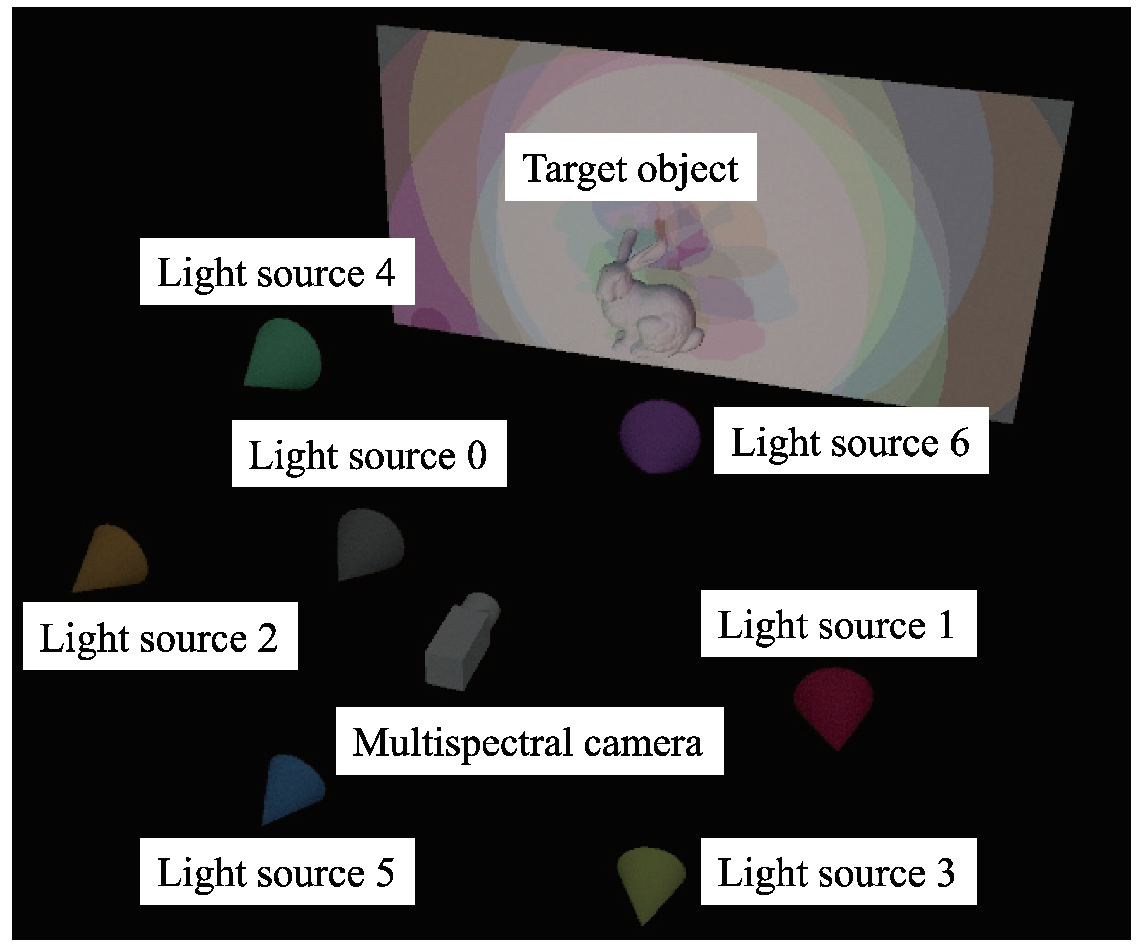
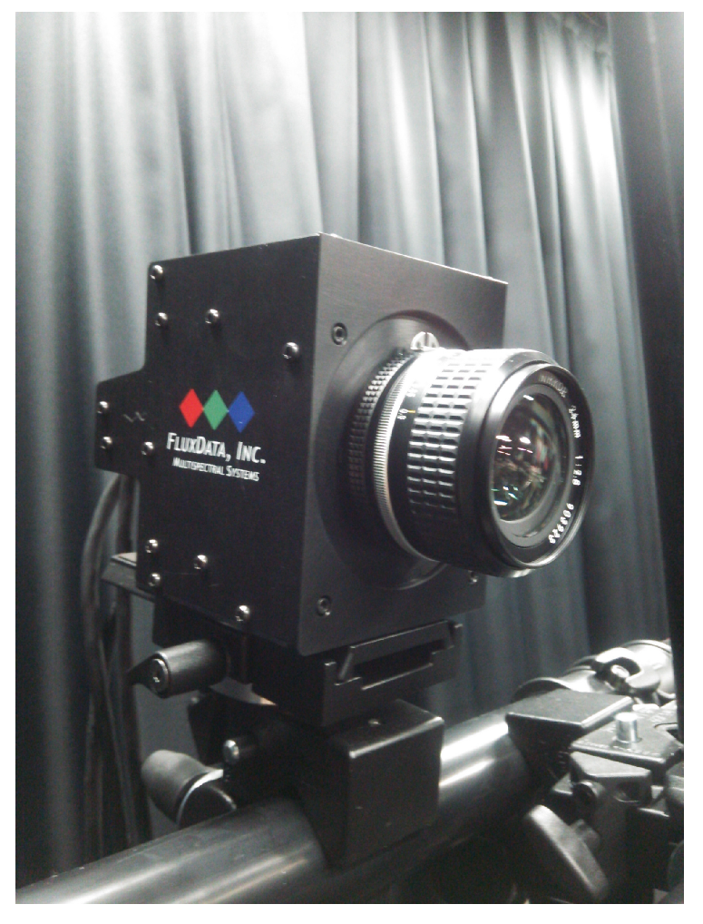
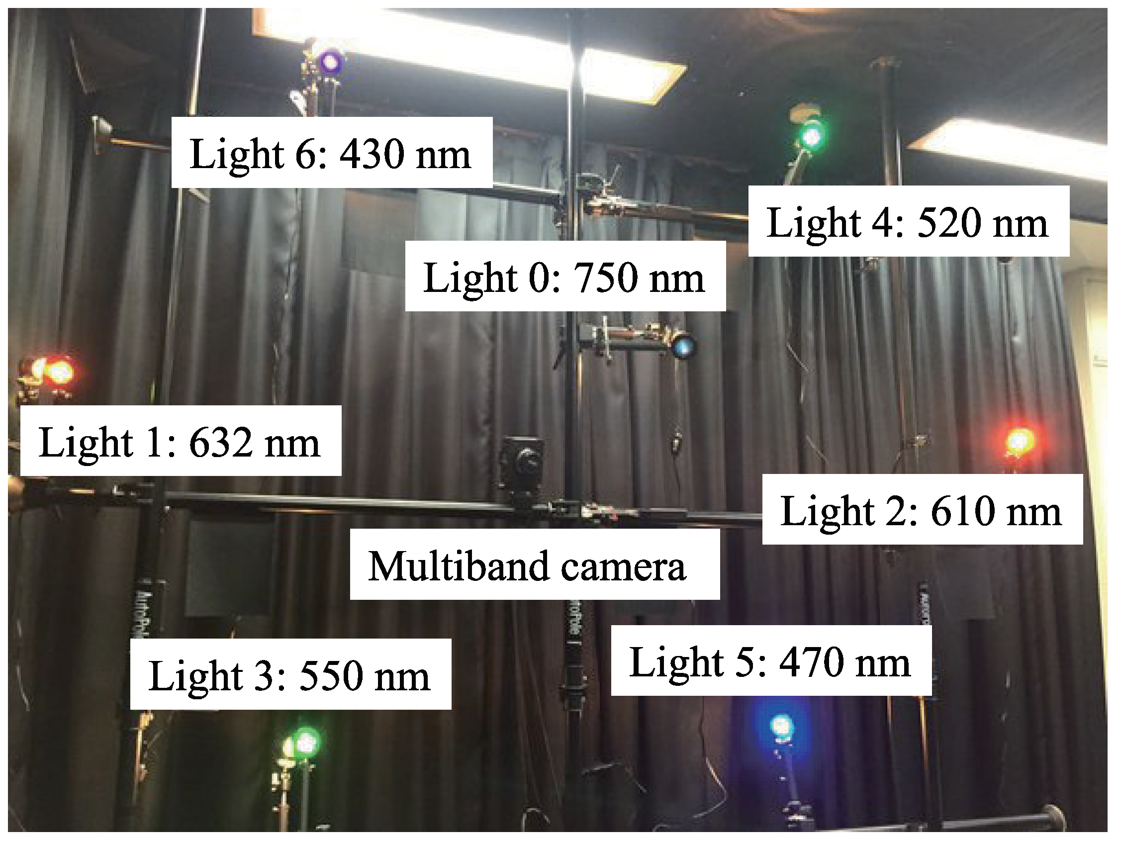
4.1. Experimental Setup
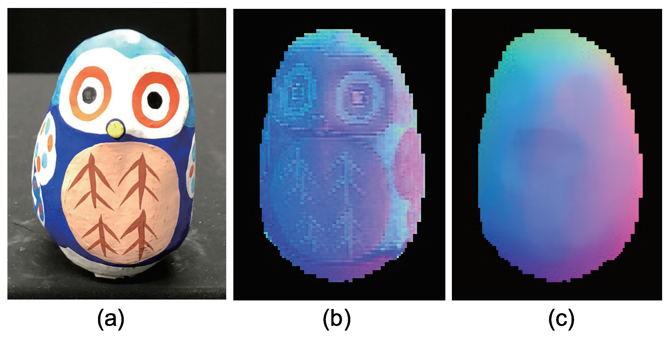
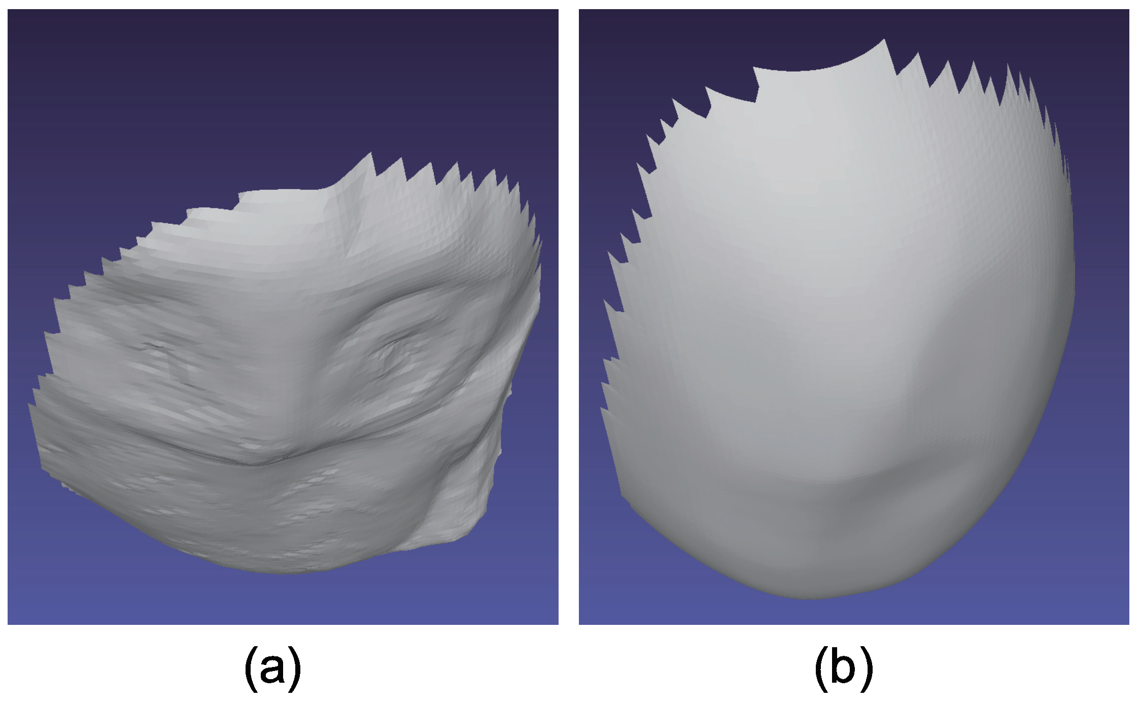
4.2. Experimental Result
4.3. Discussion
5. Conclusions
Author Contributions
Funding
Acknowledgments
Conflicts of Interest
References
- Silver, W.M. Determining Shape and Reflectance Using Multiple Images. Master’s Thesis, Massachusetts Institute of Technology, Cambridge, MA, USA, 1980. [Google Scholar]
- Woodham, R.J. Photometric method for determining surface orientation from multiple images. Opt. Eng. 1980, 19, 139–144. [Google Scholar] [CrossRef]
- Drew, M.; Kontsevich, L. Closed-form attitude determination under spectrally varying illumination. In Proceedings of the IEEE Conference on Computer Vision and Pattern Recognition, Seattle, WA, USA, 21–23 June 1994; pp. 985–990. [Google Scholar]
- Kontsevich, L.; Petrov, A.; Vergelskaya, I. Reconstruction of shape from shading in color images. J. Opt. Soc. Am. A 1994, 11, 1047–1052. [Google Scholar] [CrossRef]
- Woodham, R.J. Gradient and curvature from photometric stereo including local confidence estimation. J. Opt. Soc. Am. 1994, 11, 3050–3068. [Google Scholar] [CrossRef]
- Anderson, R.; Stenger, B.; Cipolla, R. Color photometric stereo for multicolored surfaces. In Proceedings of the International Conference on Computer Vision, Barcelona, Spain, 6–13 November 2011; pp. 2182–2189. [Google Scholar]
- Brostow, G.J.; Stenger, B.; Vogiatzis, G.; Hernández, C.; Cipolla, R. Video normals from colored lights. IEEE Trans. Pattern Anal. Mach. Intell. 2011, 33, 2104–2114. [Google Scholar] [CrossRef] [PubMed]
- Chakrabarti, A.; Sunkavalli, K. Single-image RGB photometric stereo with spatially-varying albedo. In Proceedings of the International Conference on 3D Vision, Stanford, CA, USA, 25–28 October 2016; pp. 258–266. [Google Scholar]
- Drew, M.S. Reduction of rank-reduced orientation-from-color problem with many unknown lights to two-image known-illuminant photometric stereo. In Proceedings of the International Symposium on Computer Vision, Coral Gables, FL, USA, 21–23 November 1995; pp. 419–424. [Google Scholar]
- Drew, M.S. Direct solution of orientation-from-color problem using a modification of Pentland’s light source direction estimator. Comput. Vis. Image Understand. 1996, 64, 286–299. [Google Scholar] [CrossRef]
- Drew, M.S.; Brill, M.H. Color from shape from color: A simple formalism with known light sources. J. Opt. Soc. Am. A 2000, 17, 1371–1381. [Google Scholar] [CrossRef]
- Fyffe, G.; Yu, X.; Debevec, P. Single-shot photometric stereo by spectral multiplexing. In Proceedings of the IEEE International Conference on Computational Photography, Pittsburgh, PA, USA, 8–10 April 2011; pp. 1–6. [Google Scholar]
- Hernandez, C.; Vogiatzis, G.; Brostow, G.J.; Stenger, B.; Cipolla, R. Non-rigid photometric stereo with colored lights. In Proceedings of the IEEE International Conference on Computer Vision, Rio de Janeiro, Brazil, 14–21 October 2007; p. 8. [Google Scholar]
- Hernández, C.; Vogiatzis, G.; Cipolla, R. Shadows in three-source photometric stereo. In Proceedings of the ECCV 2008, Marseille, France, 12–18 October 2008; pp. 290–303. [Google Scholar]
- Jiao, H.; Luo, Y.; Wang, N.; Qi, L.; Dong, J.; Lei, H. Underwater multi-spectral photometric stereo reconstruction from a single RGBD image. In Proceedings of the Asia-Pacific Signal and Information Processing Association Annual Summit and Conference, Jeju, South Korea, 13–16 December 2016; pp. 1–4. [Google Scholar]
- Kim, H.; Wilburn, B.; Ben-Ezra, M. Photometric stereo for dynamic surface orientations. In Proceedings of the European Conference on Computer Vision, LNCS 6311, Crete, Greece, 5–11 Septermber 2010; pp. 59–72. [Google Scholar]
- Landstrom, A.; Thurley, M.J.; Jonsson, H. Sub-millimeter crack detection in casted steel using color photometric stereo. In Proceedings of the International Conference on Digital Image Computing: Techniques and Applications, Hobart, TAS, Australia, 26–28 November 2013; pp. 1–7. [Google Scholar]
- Petrov, A.P.; Kontsevich, L.L. Properties of color images of surfaces under multiple illuminants. J. Opt. Soc. Am. A 1994, 11, 2745–2749. [Google Scholar] [CrossRef]
- Rahman, S.; Lam, A.; Sato, I.; Robles-Kelly, A. Color photometric stereo using a rainbow light for non-Lambertian multicolored surfaces. In Proceedings of the Asian Conference on Computer Vision, Singapore, 1–5 November 2014; pp. 335–350. [Google Scholar]
- Roubtsova, N.; Guillemaut, J.Y. Colour Helmholtz stereopsis for reconstruction of complex dynamic scenes. In Proceedings of the International Conference on 3D Vision, Tokyo, Japan, 8–11 December 2014; pp. 251–258. [Google Scholar]
- Vogiatzis, G.; Hernández, C. Practical 3d reconstruction based on photometric stereo. In Computer Vision: Detection, Recognition and Reconstruction; Cipolla, R., Battiato, S., Farinella, G.M., Eds.; Springer: Berlin/Heidelberg, Germany, 2010; pp. 313–345. [Google Scholar]
- Vogiatzis, G.; Hernandez, C. Self-calibrated, multi-spectral photometric stereo for 3D face capture. Int. J. Comput. Vis. 2012, 97, 91–103. [Google Scholar] [CrossRef]
- Gotardo, P.F.U.; Simon, T.; Sheikh, Y.; Mathews, I. Photogeometric scene flow for high-detail dynamic 3D reconstruction. In Proceedings of the IEEE International Conference on Computer Vision, Santiago, Chile, 7–13 December 2015; pp. 846–854. [Google Scholar]
- Nicodemus, F.E.; Richmond, J.C.; Hsia, J.J.; Ginsberg, I.W.; Limperis, T. Geometrical considerations and nomenclature of reflectance. In Radiometry; Wolff, L.B., Shafer, S.A., Healey, G., Eds.; Jones and Bartlett Publishers, Inc.: Boston, MA, USA, 1992; pp. 940–945. [Google Scholar]
- Quéau, Y.; Mecca, R.; Durou, J.-D. Unbiased photometric stereo for colored surfaces: A variational approach. In Proceedings of the IEEE Conference on Computer Vision and Pattern Recognition, Las Vegas, NV, USA, 27–30 June 2016; pp. 4359–4368. [Google Scholar]
- Oswald, M.R.; Töppe, E.; Cremers, D. Fast and globally optimal single view reconstruction of curved objects. In Proceedings of the IEEE Conference on Computer Vision and Pattern Recognition, Providence, RI, USA, 16–21 June 2012; pp. 534–541. [Google Scholar]
- Quéau, Y.; Durou, J.-D.; Aujol, J.-F. Normal integration: A survey. J. Math. Imaging Vis. 2018, 60, 576–593. [Google Scholar] [CrossRef]
- Horn, B.K.P.; Brooks, M.J. The variational approach to shape from shading. Comput. Vis. Graph. Image Process. 1986, 33, 174–208. [Google Scholar] [CrossRef]
- Ikeuchi, K.; Horn, B.K.P. Numerical shape from shading and occluding boundaries. Artif. Intell. 1981, 17, 141–184. [Google Scholar] [CrossRef]
- Frankot, R.T.; Chellappa, R. A method for enforcing integrability in shape from shading algorithms. IEEE Trans. Pattern Anal. Mach. Intell. 1988, 10, 439–451. [Google Scholar] [CrossRef]
- Bähr, M.; Breuß, M.; Quéu, Y.; Boroujerdi, A.S.; Durou, J.-D. Fast and accurate surface normal integration on non-rectangular domains. Comput. Vis. Media 2017, 3, 107–129. [Google Scholar] [CrossRef]
- Barnard, K.; Ciurea, F.; Funt, B. Sensor sharpening for computational color constancey. J. Opt. Soc. Am. A 2001, 18, 2728–2743. [Google Scholar] [CrossRef]
- Finlayson, G.D. Spectral sharpening: Sensor transformations for improved color constancey. J. Opt. Soc. Am. A 1994, 11, 1553–1563. [Google Scholar] [CrossRef]
- Kawakami, R.; Ikeuchi, K. Color estimation from a single surface color. In Proceedings of the IEEE Conference on Computer Vision and Pattern Recognition, Miami, FL, USA, 20–25 June 2009; pp. 635–642. [Google Scholar]
- Sun, J.; Smith, M.; Smith, L.; Midha, S.; Bamber, J. Object surface recovery using a multi-light photometric stereo technique for non-Lambertian surfaces subject to shadows and specularities. Image Vis. Comput. 2007, 25, 1050–1057. [Google Scholar] [CrossRef]
- Quéau, Y.; Mecca, R.; Durou, J.-D.; Descombes, X. Photometric stereo with only two image: A theoretical study and numerical solution. Image Vis. Comput. 2017, 57, 175–191. [Google Scholar] [CrossRef][Green Version]


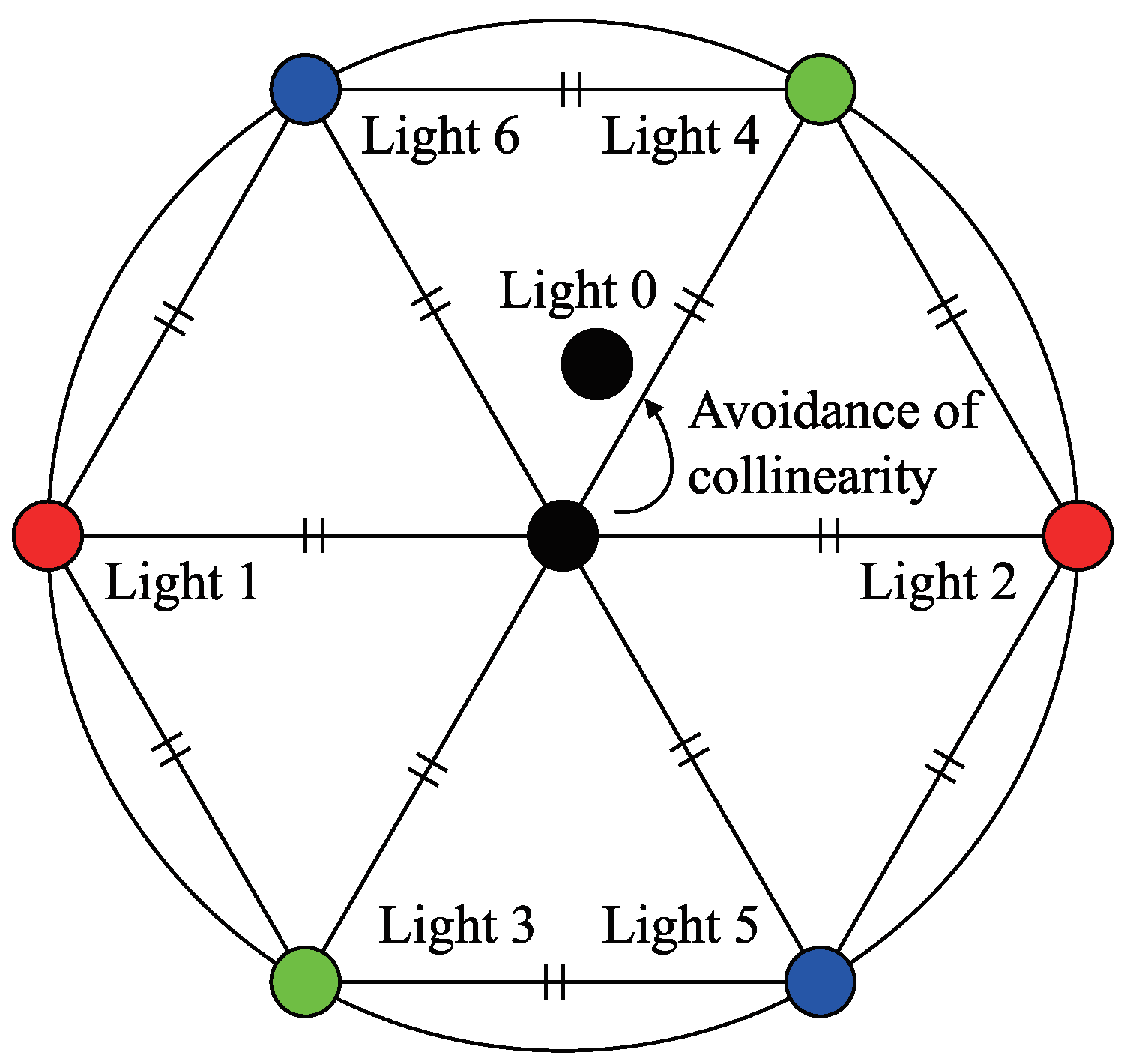
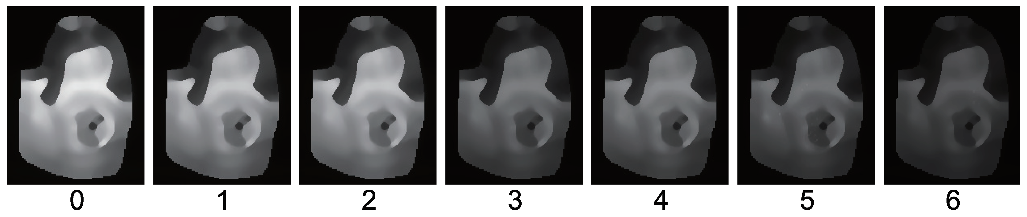
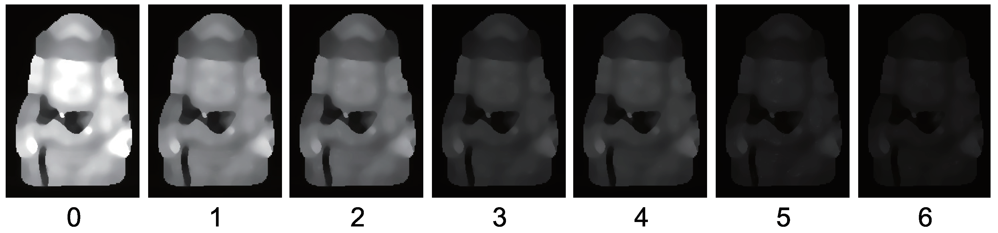
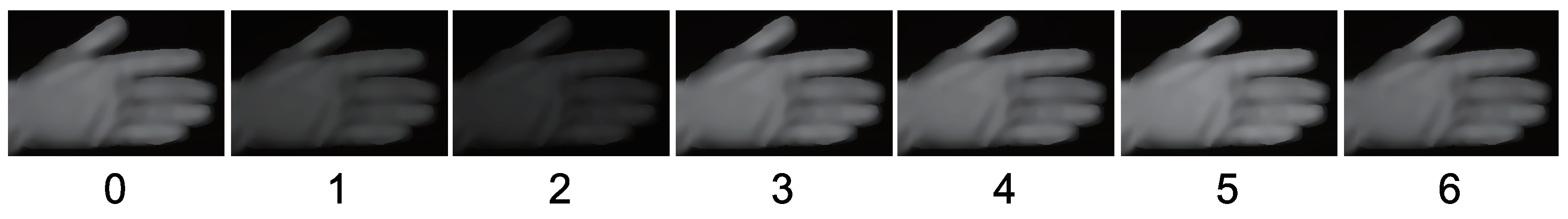
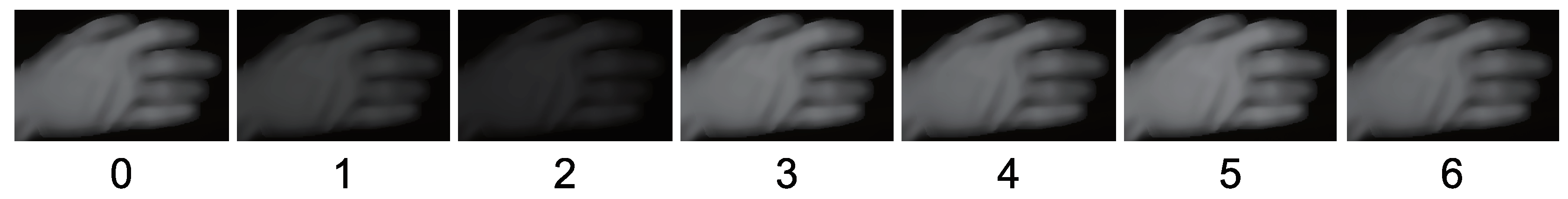
| Light | 0 | 1 | 2 | 3 | 4 | 5 | 6 |
|---|---|---|---|---|---|---|---|
| Peak | 750 nm | 632 nm | 610 nm | 550 nm | 520 nm | 470 nm | 430 nm |
| FWHM | 10 nm | 10 nm | 10 nm | 10 nm | 10 nm | 10 nm | 10 nm |
© 2019 by the authors. Licensee MDPI, Basel, Switzerland. This article is an open access article distributed under the terms and conditions of the Creative Commons Attribution (CC BY) license (http://creativecommons.org/licenses/by/4.0/).
Share and Cite
Miyazaki, D.; Onishi, Y.; Hiura, S. Color Photometric Stereo Using Multi-Band Camera Constrained by Median Filter and Occluding Boundary. J. Imaging 2019, 5, 64. https://doi.org/10.3390/jimaging5070064
Miyazaki D, Onishi Y, Hiura S. Color Photometric Stereo Using Multi-Band Camera Constrained by Median Filter and Occluding Boundary. Journal of Imaging. 2019; 5(7):64. https://doi.org/10.3390/jimaging5070064
Chicago/Turabian StyleMiyazaki, Daisuke, Yuka Onishi, and Shinsaku Hiura. 2019. "Color Photometric Stereo Using Multi-Band Camera Constrained by Median Filter and Occluding Boundary" Journal of Imaging 5, no. 7: 64. https://doi.org/10.3390/jimaging5070064
APA StyleMiyazaki, D., Onishi, Y., & Hiura, S. (2019). Color Photometric Stereo Using Multi-Band Camera Constrained by Median Filter and Occluding Boundary. Journal of Imaging, 5(7), 64. https://doi.org/10.3390/jimaging5070064