A Review of Supervised Edge Detection Evaluation Methods and an Objective Comparison of Filtering Gradient Computations Using Hysteresis Thresholds

Abstract

Useful for human visual perception, edge detection remains a crucial stage in numerous image processing applications. One of the most challenging goals in contour detection is to operate algorithms that can process visual information as humans require. To ensure that an edge detection technique is reliable, it needs to be rigorously assessed before being used in a computer vision tool. This assessment corresponds to a supervised evaluation process to quantify differences between a reference edge map and a candidate, computed by a performance measure/criterion. To achieve this task, a supervised evaluation computes a score between a ground truth edge map and a candidate image. This paper presents a survey of supervised edge detection evaluation methods. Considering a ground truth edge map, various methods have been developed to assess a desired contour. Several techniques are based on the number of false positive, false negative, true positive and/or true negative points. Other methods strongly penalize misplaced points when they are outside a window centered on a true or false point. In addition, many approaches compute the distance from the position where a contour point should be located. Most of these edge detection assessment methods will be detailed, highlighting their drawbacks using several examples. In this study, a new supervised edge map quality measure is proposed. The new measure provides an overall evaluation of the quality of a contour map by taking into account the number of false positives and false negatives, and the degrees of shifting. Numerous examples and experiments show the importance of penalizing false negative points differently than false positive pixels because some false points may not necessarily disturb the visibility of desired objects, whereas false negative points can significantly change the aspect of an object. Finally, an objective assessment is performed by varying the hysteresis thresholds on contours of real images obtained by filtering techniques. Theoretically, by varying the hysteresis thresholds of the thin edges obtained by filtering gradient computations, the minimum score of the measure corresponds to the best edge map, compared to the ground truth. Twenty-eight measures are compared using different edge detectors that are robust or not robust regarding noise. The scores of the different measures and different edge detectors are recorded and plotted as a function of the noise level in the original image. The plotted curve of a reliable edge detection measure must increase monotonously with the noise level and a reliable edge detector must be less penalized than a poor detector. In addition, the obtained edge map tied to the minimum score of a considered measure exposes the reliability of an edge detection evaluation measure if the edge map obtained is visually closer to the ground truth or not. Hence, experiments illustrate that the desired objects are not always completely visible using ill-suited evaluation measure.

1. Introduction: Edge Detection and Hysteresis Thresholding

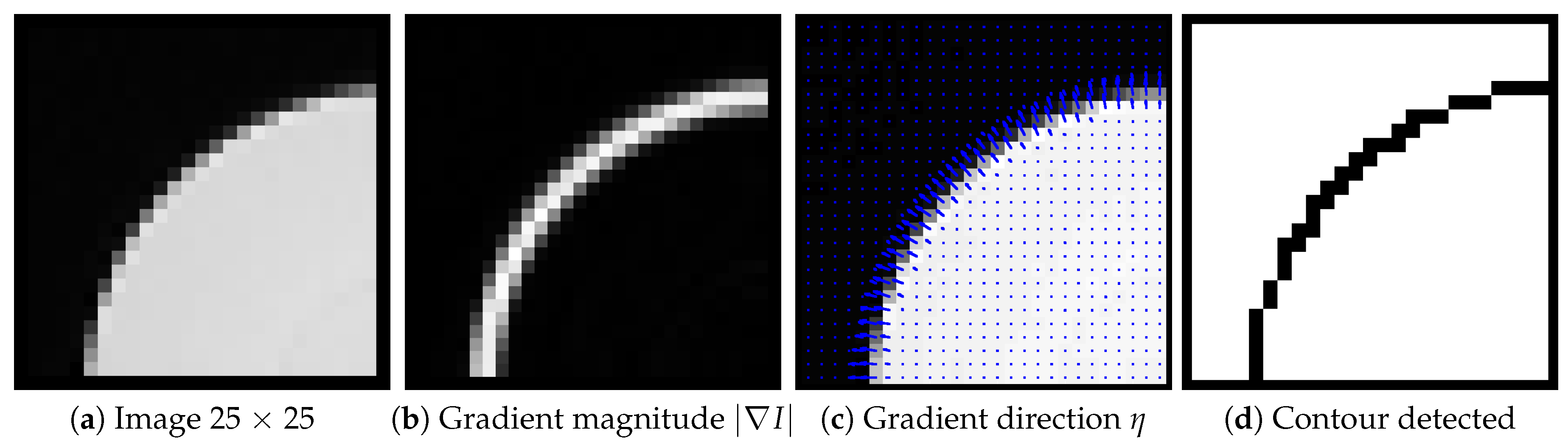
A digital image is a discrete representation of a real and continuous world. Each point of an image, i.e., pixel, quantifies a piece or pieces of gray-scale, brightness or color information. The transition between dark and bright pixels corresponds to contours. They are essential information for the interpretation and exploitation of images. Edge detection is an important field and one of the oldest topics in image processing because the process frequently attempts to capture the most important structures in the image [1]. Edge detection is therefore a fundamental step in computer vision approaches. Furthermore, edge detection could itself be used to qualify a region segmentation technique. Additionally, the edge detection assessment remains very useful in image segmentation, registration, reconstruction or interpretation. It is hard to design an algorithm that is able to detect the exact edge from an image with good localization and orientation. In the literature, various techniques have emerged and, due to its importance, edge detection continues to be an active research area [2]. The detection is based on the local geometric properties of the considered image by searching for intensity variation in the gradient direction [1]. There are two main approaches for contour detection: first-order derivative [3,4,5,6,7] or second-order [8]. The best-known and most useful edge detection methods are based on gradient computing first-order fixed operators [3,4]. Oriented first-order operators compute the maximum energy in an orientation [9,10,11] or two directions [12]. As illustrated in Figure 1, typically, these methods consist of three steps:

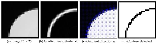
Figure 1. Example of edge detection on an image. In (c), arrows representing $\eta$ are pondered by $|\nabla I|$.

• Computation of the gradient magnitude $|\nabla I|$ and its orientation $\eta$, see Table 1, using a 3 × 3 templates [3], the first derivative of the filter (vertical and horizontal [4]), steerable Gaussian filters, oriented anisotropic Gaussian kernels or combination of two half Gaussian kernels.
  Table 1. Gradient magnitude and orientation computation for a scalar image I, where $I_{\theta }$ represents the image derivative using a first-order filter at the $\theta$ orientation (in radians).

  Type of Operator	Fixed Operator [3,4,5,6,7]	Oriented Filters [9,10,11]	Half Gaussian Kernels [12]
  Gradient magnitude	$|\nabla I|=\sqrt{I_0^2+I_{\pi /2}^2}$	$|\nabla I|={\displaystyle \underset{\theta \in \left[0,\pi \right[}{max}}|I_{\theta }|$	$|\nabla I|={\displaystyle \underset{\theta \in \left[0,2\pi \right[}{max}}{I}_{\theta }-{\displaystyle \underset{\theta \in \left[0,2\pi \right[}{min}}{I}_{\theta }$
  Gradient direction	$\eta =arctan\left({\displaystyle \frac{I_{\pi /2}}{I_0}}\right)$	$\eta ={\displaystyle \underset{\theta \in \left[0,\pi \right[}{argmax}}|I_{\theta }|+{\displaystyle \frac{\pi }{2}}$	$\eta =\left({\displaystyle \underset{\theta \in \left[0,2\pi \right[}{argmax}}{I}_{\theta }+{\displaystyle \underset{\theta \in \left[0,2\pi \right[}{argmin}}{I}_{\theta }\right)/2$

• Non-maximum suppression to obtain thin edges: the selected pixels are those having gradient magnitude at a local maximum along the gradient direction $\eta$, which is perpendicular to the edge orientation [4].
• Thresholding of the thin contours to obtain an edge map.

Table 1 gives the different possibilities for gradient and its associated orientations involving several edge detection algorithms compared in this paper.

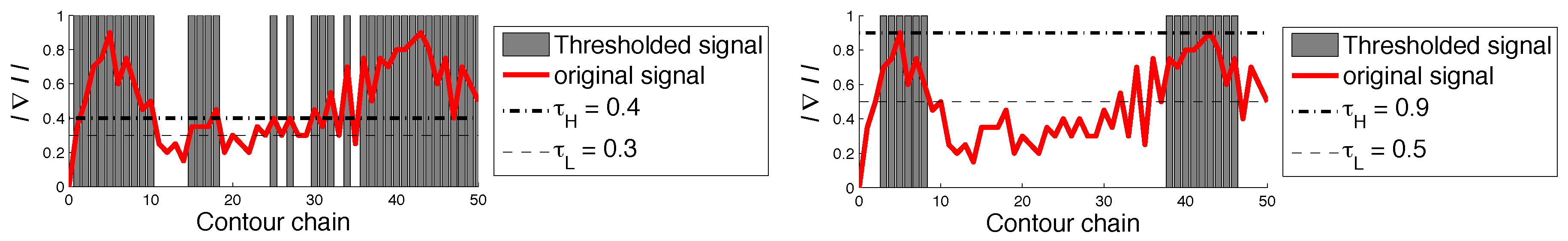
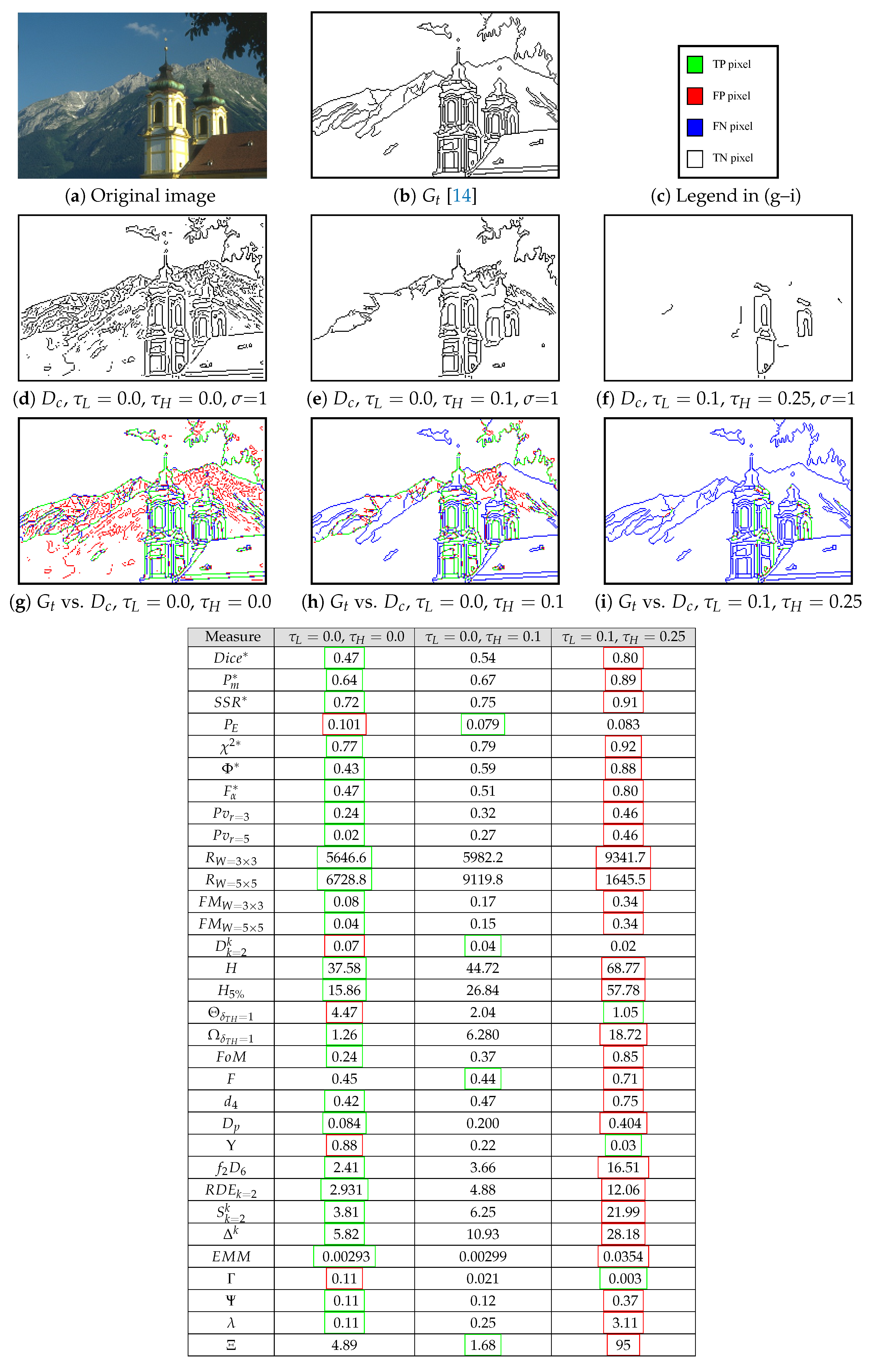
The final step remains a difficult stage in image processing, but it is a crucial operation for comparing several segmentation algorithms. Unfortunately, it is far from straightforward to choose an ideal threshold value to detect the edges of the desirable features. Usually, a threshold is fixed in a function of the objects’ contours, which must be visible, but this is not an objective segmentation for the evaluation. Otherwise, in edge detection, the hysteresis process uses the connectivity information of the pixels belonging to thin contours and thus remains a more elaborated method than binary thresholding [4]. To put it simply, this technique determines a contour image that has been thresholded at different levels (low: ${\tau }_L$ and high: ${\tau }_H$). The low threshold ${\tau }_L$ determines which pixels are considered as edge points if at least one point higher than ${\tau }_H$ exists in a contour chain where all the pixel values are also higher than ${\tau }_L$, as represented with a signal in Figure 2. Segmented real images using hysteresis thresholds are presented, later in this paper, in Figure 11. On the one hand, this algorithm is able to partly detect blurred edges of an object. On the other hand, the lower the thresholds are, the more the undesirable pixels are preserved and the problem remains that thresholds are fixed for both the segmentation and the evaluation.

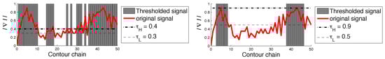
Figure 2. Example of hysteresis threshold applied along a contour chain.

In order to compare the quality of the results by different methods, they need to render binary edge maps. This normally requires a manual process of threshold selection aimed at maximizing the quality of the results by each of the contending methods. However, this assessment suffers from a major drawback: segmentations are compared using the (deliberately) chosen threshold, and this evaluation is very subjective and not reproducible. The aim is therefore to use the dissimilarity measures without any user intervention for an objective assessment. Finally, to consider a valuable edge detection assessment, the evaluation process should produce a result that correlates with the perceived quality of the edge image, which relies on human judgment [13,14,15]. In other words, a reliable edge map should characterize all the relevant structures of an image as closely as possible, without any disappearance of desired contours. In addition, a minimum of spurious pixels should be created by the edge detector, disturbing at the same time the visibility of the main/desired objects to be detected.

In this paper, a novel technique is presented to compare edge detection techniques by using hysteresis thresholds in a supervised way, consistent with the visual perception of a human being. Comparing a ground truth contour map with an ideal edge map, several assessments can be compared by varying the parameters of the hysteresis thresholds. This study shows the importance of more strongly penalizing false negative points than false positive points, leading to a new edge detection evaluation algorithm. The experiment using synthetic and real images demonstrated that the proposed method obtains contour maps closer to the ground truth without requiring tuning parameters, and objectively outperforms other assessment methods.

2. Supervised Measures for Image Contour Evaluations

In the last 40 years, several edge detectors have been developed for digital images. Depending on their applications, with different difficulties such as noise, blur or textures in images, the best edge detector must be selected for a given task. An edge detector therefore needs to be carefully tested and assessed to study the influence of the input parameters. The measurement process can be classified as either an unsupervised or a supervised evaluation criterion. The first class of methods exploits only the input contour image and gives a coherence score that qualifies the result given by the algorithm [15]. For example, two desirable qualities are measured in [16,17]: continuation and thinness of edges; for continuation, two connected pixels of a contour must have almost identical gradient direction ($\eta$). In addition, the connectivity, i.e., how contiguous and connected edge pixels are, is evaluated in [18]. These approaches obtain a segmentation that could generally be well interpreted in image processing tasks. Even though the segmentation includes continuous, thin and contiguous edges, it does not enable evaluation of whether the segmentation result is close to or far from a desired contour. A supervised evaluation criterion computes a dissimilarity measure between a segmentation result and a ground truth, generally obtained from synthetic data or expert judgement (i.e., manual segmentation). Pioneer works in edge detection assessments were directly applicable only to vertical edges [19,20] (examples for [19] are available in [21]). Another method [22] considers either vertical contours or closed forms, pixels of contour chains connected to the true contour. Contours inside or outside the closed form are treated differently. Alternatively, authors in [23] propose an edge detector performance evaluation method in the context of image compression according to a mean square difference between the reconstructed image and the original uncompressed one. Various supervised methods have been proposed in the literature to assess different shapes of edges [21,24,25,26], the majority are detailed in this study, and more precisely in an objective way using hysteresis thresholds. In this paper, the closer to 0 the score of the evaluation is, the more the segmentation is qualified as good. Several measures are presented with respect to this property. This work focusses on comparisons of supervised edge detection evaluations in an objective way and proposes a new measure, aimed at achieving an objective assessment.

2.1. Error Measures Involving Only Statistics

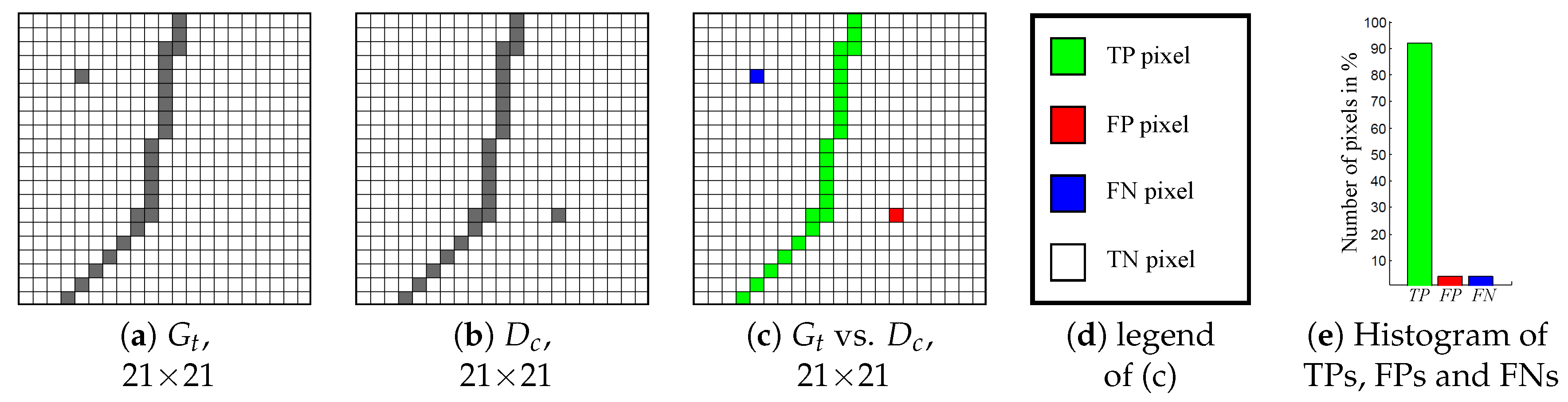
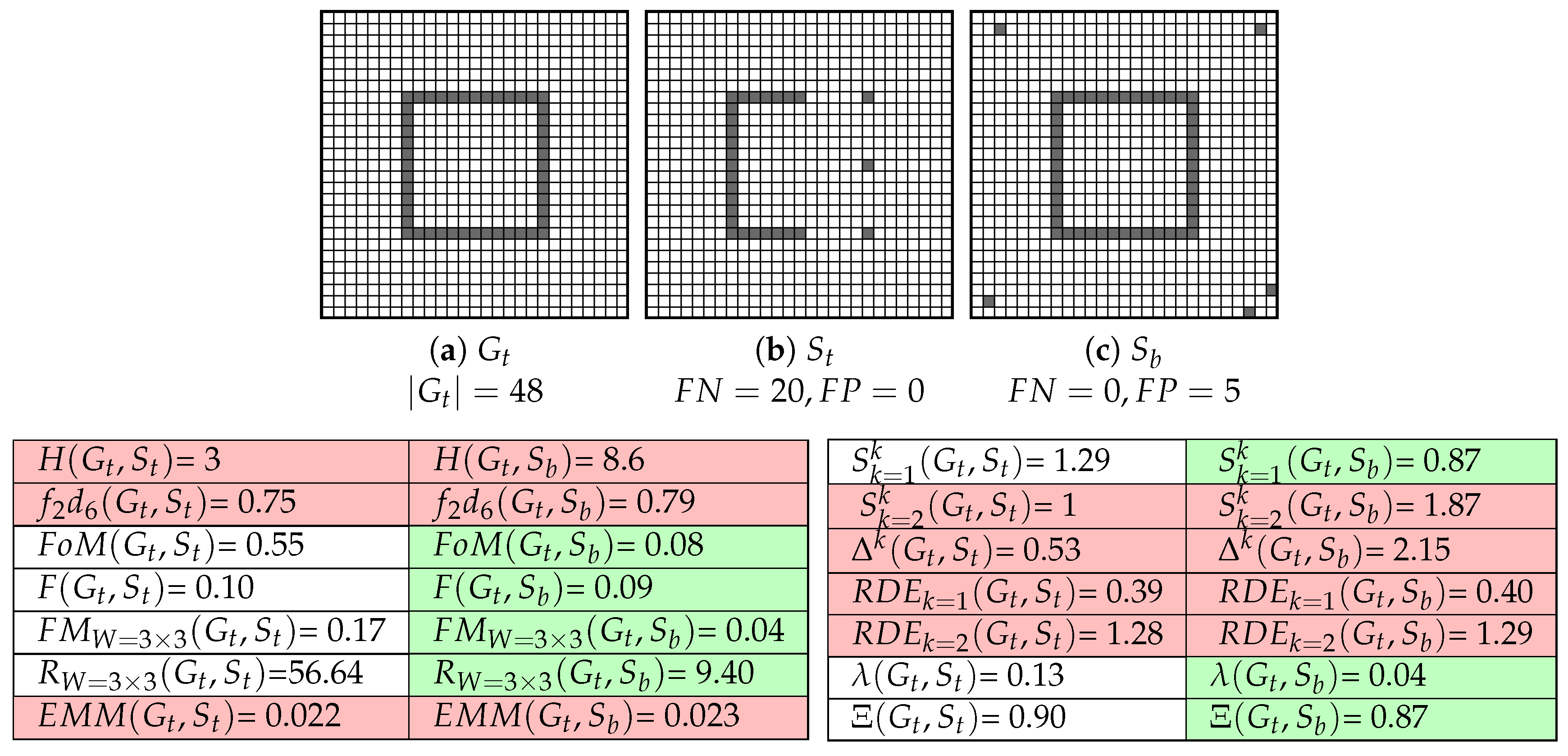
To assess an edge detector, the confusion matrix remains a cornerstone in boundary detection evaluation methods. Let $G_t$ be the reference contour map corresponding to ground truth and $D_c$ the detected contour map of an original image I. Comparing pixel per pixel $G_t$ and $D_c$, the 1st criterion to be assessed is the common presence of edge/non-edge points. A basic evaluation is composed of statistics; to that end, $G_t$ and $D_c$ are combined. Afterwards, denoting $|·|$ as the cardinality of a set, all points are divided into four sets (see Figure 3):

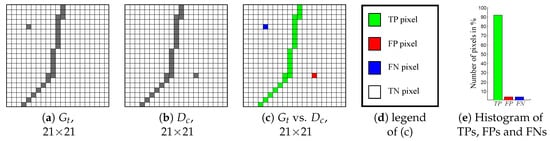
Figure 3. Example of ground truth ($G_t$) versus (vs.) a desired contour ($D_c$).

• True Positive points (TPs), common points of $G_t$ and $D_c$:          $TP=\left|G_t\cap D_c\right|$,
• False Positive points (FPs), spurious detected edges of $D_c$:        $FP=\left|\neg G_t\cap D_c\right|$,
• False Negative points (FNs), missing boundary points of $D_c$:    $FN=\left|G_t\cap \neg D_c\right|$,
• True Negative points (TNs), common non-edge points:               $TN=\left|\neg G_t\cap \neg D_c\right|$.

Figure 3 presents an example of $G_t$ and $D_c$. Comparing these two images, there are 23 TPs, one FN and one FP. Other examples are presented in Figure 10 comparing different $D_c$ with the same $G_t$.

Several edge detection evaluations involving confusion matrices are presented in Table 2. Computing only FPs and FNs or their sum enables a segmentation assessment to be performed and several edge detectors to be compared [12]. On the contrary, TPs are an indicator, as for Absotude Grading ($A_G$) and $SSR$; these two formulae are nearly the same, just a square root of difference, so they behave absolutely similarly. The Performance measure ($P_m$, also known as Jaccard coefficient [27]) or $Dice$ directly and simultaneously considers the three entities $TP$, $FP$ and $FN$ to assess a binary image. It decreases with improved quality of detection. Note that $|G_t|=TP+FN$ and that $|D_c|=TP+FP$, so it is easy to observe that $Dic{e}^{\ast }$, $A_G\ast$, $SS{R}^{\ast }$ and $P_m^{\ast }$ behave similarly when $FN$ and/or $FP$ increase (more details in [21]), as shown in the experimental results. Moreover, considering the original versions of $Dice$ and $P_m$ are widely utilized for medical images assessments, they are related by $Dice=\frac{2·|G_t\cap D_c|}{|G_t|+|D_c|}=\frac{2·|G_t\cap D_c|}{|G_t\cup D_c|}/\left(1+\frac{|G_t\cap D_c|}{|G_t\cup D_c|}\right)=\frac{2·P_m}{P_m+1}$. In addition, $Localization-error$ ($P_E$) and $Misclassification$ $Error$ ($ME$) represent the same measurement. Indeed, as $|I|=TP+TN+FP+FN$, the $ME$ measure can be rewritten as:

$$ME\left(G_t,D_c\right)=1-{\displaystyle \frac{TP+TN}{TN+FN+TP+FP}}={\displaystyle \frac{TN+FN+TP+FP}{TN+FN+TP+FP}}-{\displaystyle \frac{TP+TN}{TN+FN+TP+FP}}=P_E.$$

Table 2. List of error measures involving only statistics.

Complemented $Dice$ measure [28]	$Dic{e}^{\ast }=1-{\displaystyle \frac{2·TP}{2·TP+FN+FP}}$
Complemented $Performance$ $measure$ [29,30,31,32]	$P_m^{\ast }\left(G_t,D_c\right)=1-{\displaystyle \frac{TP}{|G_t\cup D_c|}}=1-{\displaystyle \frac{TP}{TP+FP+FN}}$
Complemented Absolute Grading [33]	$A_G^{\ast }=1-{\displaystyle \frac{TP}{\sqrt{\left|G_t\right|·\left|D_c\right|}}}=1-{\displaystyle \frac{TP}{\sqrt{\left(TP+FN\right)·\left(TP+FP\right)}}}$
Complemented Segmentation Success Ratio [34]	$SS{R}^{\ast }=1-{\displaystyle \frac{T{P}^2}{\left|G_t\right|·\left|D_c\right|}}=1-{\displaystyle \frac{T{P}^2}{\left(TP+FN\right)·\left(TP+FP\right)}}$
$Localization-error$ [35]	$P_E\left(G_t,D_c\right)={\displaystyle \frac{FP+FN}{|I|}}$
$Misclassification$ $Error$ [36]	$ME\left(G_t,D_c\right)=1-{\displaystyle \frac{TP+TN}{TN+FN+TP+FP}}$
Complemented $\mathsf{\Phi }$ measure [37]	${\mathsf{\Phi }}^{\ast }\left(G_t,D_c\right)=1-{\displaystyle \frac{TPR·TN}{TN+FP}}$
Complemented ${\chi }^2$ measure [38]	${\chi }^{2\ast }\left(G_t,D_c\right)=1-{\displaystyle \frac{TPR-TP-FP}{1-TP-FP}·\frac{TP+FP+FPR}{TP+FP}}$
Complemented $F_{\alpha }$ measure [39]	$F_{\alpha }^{\ast }\left(G_t,D_c\right)=1-{\displaystyle \frac{P\mathrm{REC}·TPR}{\alpha ·TPR+(1-\alpha )·P\mathrm{REC}}}$, with $\alpha \in ]0;1]$

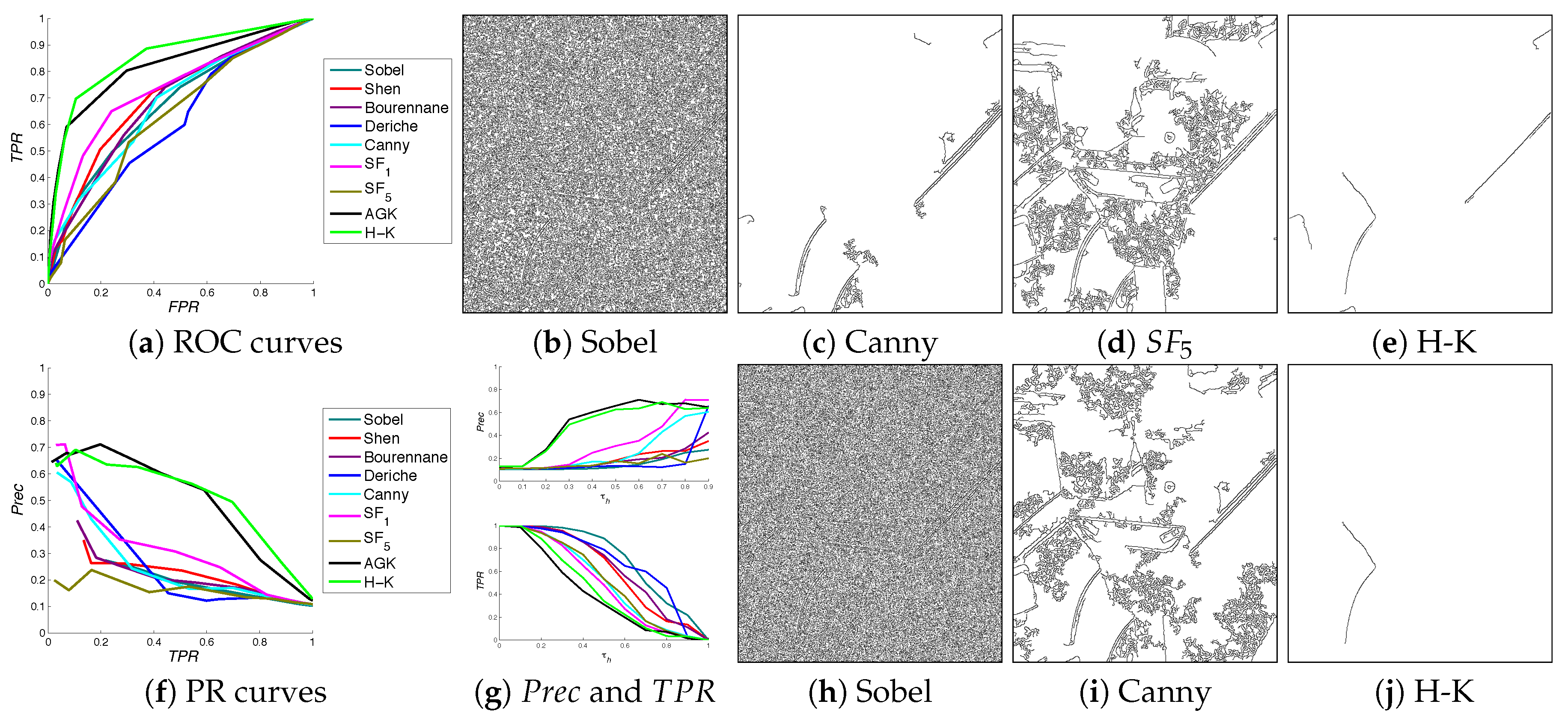
Another way to display evaluations is to create Receiver Operating Characteristic (ROC) [40] curves, involving True Positive Rates ($TPR$) and False Positive Rates ($FPR$):

$$TPR=\frac{TP}{TP+FN}\mathrm{and}FPR=\frac{FP}{FP+TN}.$$

(1)

Then, $TPR$ is plotted versus (vs.) $FPR$ by varying the threshold of the detector (see Figure 4 (Section 4 details filters)). The closer the area under the curve is to 1, the better the segmentation, and an area of 1 represents a perfect edge detection. Finally, the score higher than and furthest from the diagonal (i.e., line from (0, 0) to (1, 1)) of ROC is considered as the best segmentation (here, H-K in (e) in Figure 4). However, the score of $S{F}_5$ is poor, but the segmentation seems better than Canny, Sobel and H-K for this example. Thus, any edge detectors can be called the best by simply making small changes $G_t$ or the parameter set [41]. As TNs are the majority set of pixels, Precision–Recall (PR) [39,42] does not take into account the $TN$ value by substituting $FPR$ with a precision variable: $Prec=\frac{TP}{TP+FP}$. By using both $TPR$ and $Prec$ entities, PR curves quantify more precisely than ROC curves the compromise between under-detection ($TPR$ value) and over-detection ($Prec$ value) (see Figure 4g). An example of PR curve is available in Figure 4f. The best segmentation is tied to the curve point closest to the point situated in (1, 1). As shown in Figure 4h,j, results of Sobel and H-K for PR are similar to those obtained with ROC. These evaluation types are effective for $G_t$ having precise locations of edges, as in synthetic images [14,43], since a displacement of $G_t$ or $D_c$ points strongly penalizes the segmentation.

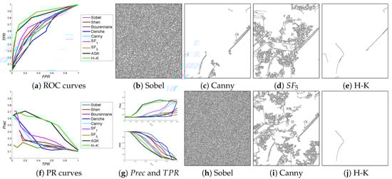
Figure 4. Receiver Operating Characteristic (ROC) and Precision–Recall (PR) curves for several edge detectors. Images in (b–e) and (h–j) represent the best segmentation for each indicated detector tied to ROC curves and PR curves, respectively. The ground truth image (parkingmeter) is available in Figure 16 and the original image in Figure 17 (Peak Signal to Noise Ratio: PSNR = 14 dB).

Derived from $TPR$ and $FPR$, the three measures $\mathsf{\Phi }$, ${\chi }^2$ and $F_{\alpha }$ (detailed in Table 2) are frequently used. The complement of these measures translates a value close to 0 as a good segmentation. Among these three measures, $F_{\alpha }$ remains the most stable because it does not consider the TNs, which are dominant in edge maps (see [14]). Indeed, taking into consideration $TN$ in $\mathsf{\Phi }$ and ${\chi }^2$ influences solely the measurement (as is the case in huge images). These measures evaluate the comparison of two edge images, pixel per pixel, tending to severely penalize an (even slightly) misplaced contour, as illustrated in Figure 8.

Consequently, some evaluations resulting from the confusion matrix recommend incorporating spatial tolerance. Tolerating a distance from the true contour and integrating several TPs for one detected contour can penalize efficient edge detection methods, or, on the contrary, benefit poor ones (especially for corners or small objects). The assessment should therefore penalize a misplaced edge point proportionally to the distance from its true location. More details are given in [21,26], some examples and comparisons are shown in [21].

2.2. Assessments Involving Spacial Areas Around Edges

2.2.1. The Performance Value $P{v}_r$

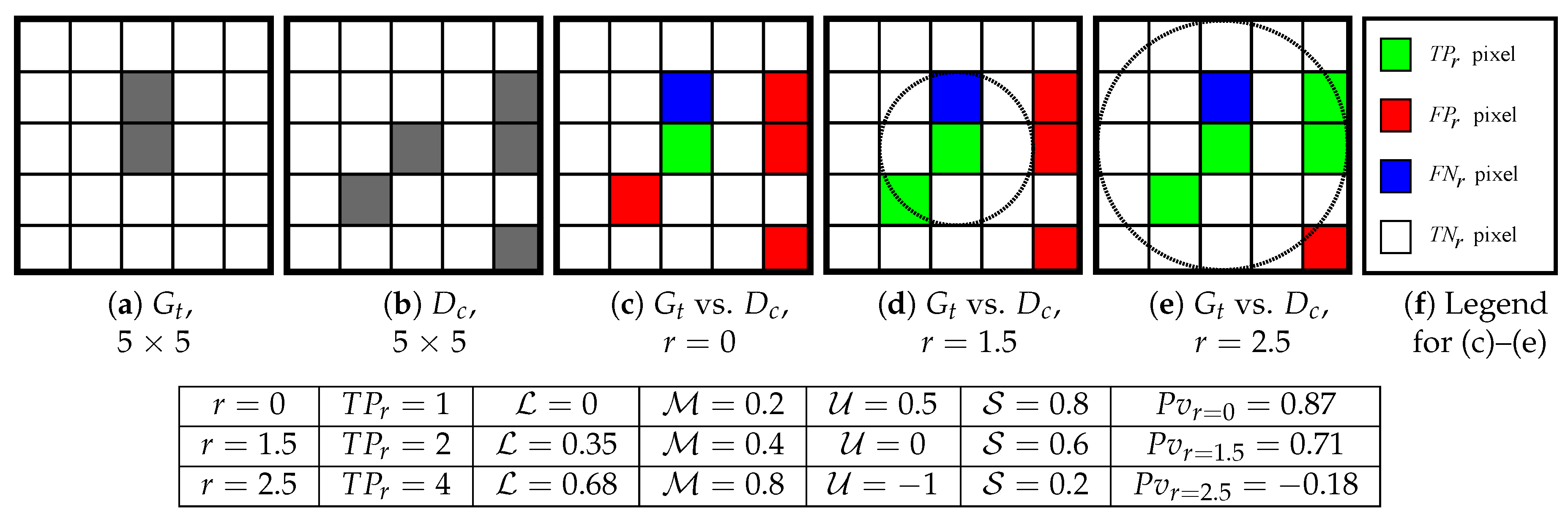
To judge the quality of segmentation results and the performance of algorithms, the performance value $P{v}_r$ in [44] combines four features: location ($\mathcal{L}$), matching ($\mathcal{M}$), unmatching ($\mathcal{U}$) and spurious ($\mathcal{S}$). In this approach, $D_c$ pixels are assimilated as TP when they belong to a disc of radius r centered on a pixel of $G_t$, as illustrated in Figure 5; this set of pixels is denoted $T{P}_r$. Thus, $F{N}_r$ represents the set of pixels of $G_t$ located at a distance (In our tests, the Euclidean distance is used, and the next section exposes different measures using distances of misplaced pixels.) higher than r of $D_c$ and, conversely, $F{P}_r$ the set of points of $D_c$ at a distance higher than r of $G_t$. The location criteria depends on the sum of the distance between each point of $T{P}_r$ and $G_t$, denoted by: ${\sum }_{p\in T{P}_r}{d}_{G_t}\left(p\right)$. Hence, the four criteria are computed as follows:

$$\left\{\begin{array}{cc}\mathcal{L}=& {\displaystyle \frac{{\sum }_{p\in T{P}_r}{d}_{G_t}\left(p\right)}{|T{P}_r|·|G_t|}},\\ \mathcal{M}=& {\displaystyle \frac{|T{P}_r|}{|D_c|}},\\ \mathcal{U}=& {\displaystyle \frac{|G_t|-|T{P}_r|}{|G_t|}}={\displaystyle \frac{F{N}_r}{|G_t|}},\\ \mathcal{S}=& {\displaystyle \frac{|D_c|-|T{P}_r|}{|D_c|}}={\displaystyle \frac{F{P}_r}{|D_c|}}.\end{array}\right.$$

(2)

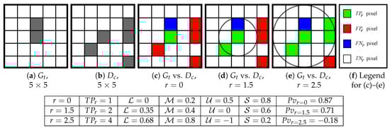
Figure 5. $Pv$ evaluation depends on the r parameter and can produce a negative evaluation. The variable r is represented by the radius of the circle in (c–e). The higher the value of r, the higher $\mathcal{L}$ and $\mathcal{M}$ are and the smaller $\mathcal{U}$ and $\mathcal{S}$ are (or can become negative for $\mathcal{U}$).

Finally, the performance value $P{v}_r$ is obtained by:

$$P{v}_r(G_t,D_c)=1-{\displaystyle \frac{\mathcal{M}}{\mathcal{M}+\mathcal{L}+\mathcal{U}+\mathcal{S}}}.$$

(3)

The main drawback of $P{v}_r$ is that the term $\frac{\mathcal{M}}{\mathcal{M}+\mathcal{L}+\mathcal{U}+\mathcal{S}}$ can obtain negative or huge values. This is explainable when $r⩾1$, we can obtain $|G_t|<|T{P}_r|$ (typically when $|G_t|<|D_c|$). Thus, $\mathcal{U}<0$; so if $|\mathcal{U}|>\mathcal{M}+\mathcal{L}+\mathcal{S}$, $P{v}_r$ could be negative, as illustrated in Figure 5. Finally, when $\mathcal{U}<0$ and $\mathcal{M}+\mathcal{L}+\mathcal{U}+\mathcal{S}\approx 0$, $P{v}_r$ tends to ± infinity (see experiments). Moreover, as illustrated in Figure 8, $P{v}_{r>1}$ obtains the same measurement for two different shapes because FPs are close to the desired contour, which is not desirable for the evaluation of small objects segmentation. Note that, when $r⩽1$, $\mathcal{L}$, and $P{v}_r$ is equivalent to $P_m^{\ast }$, since:

$$P{v}_{r⩽1}(G_t,D_c)=1-{\displaystyle \frac{TP}{{\displaystyle \frac{|D_c|·FN}{|G_t|}}+FP+TP}}.$$

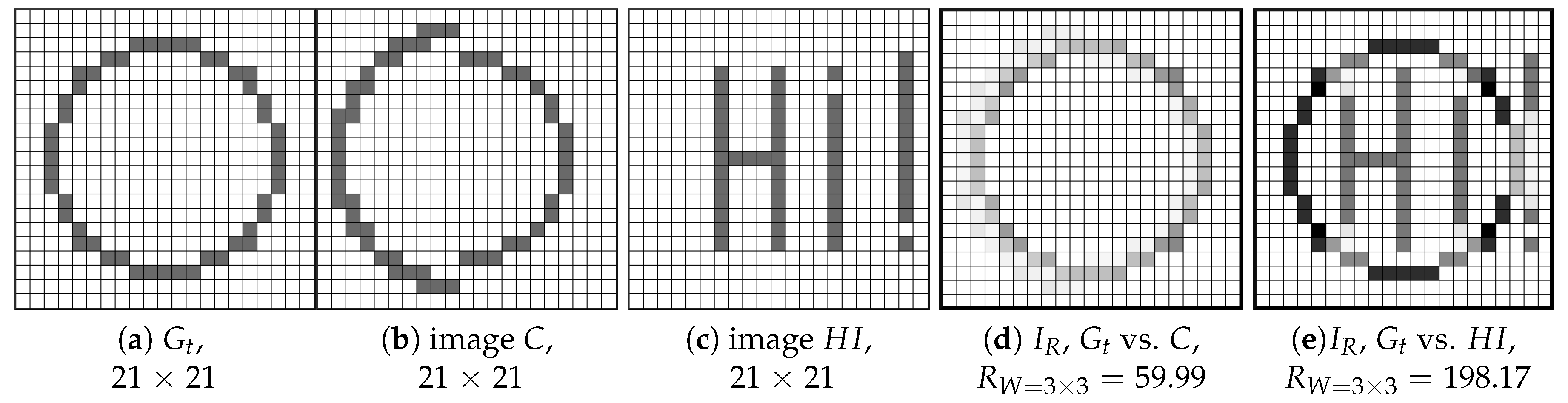
2.2.2. The Quality Measure R

In [45], a mixed measure of quality $R_W$ is presented. This evaluation depends on the number of FPs and FNs and the calculus focuses on a window W for each mistake (FP or FN). For each point of $FN$ or of $FP$, to estimate the evaluation measure $R_W$, several variables are computed:

• $n_b$, the number of FPs in W, minus the central pixel: $n_b={\displaystyle \sum _{p\in FP\cap W}}p-p_c$, with $p_c=1$ if the central pixel is a FP point, or 0 otherwise,
• $n_h$, the number of FNs in W, minus the central pixel: $n_h={\displaystyle \sum _{p\in FN\cap W}}p-p_c$, with $p_c=1$ if the central pixel is a FN point, or 0 otherwise.
• $n_e$, the number of edge points belonging to $G_t$ in W: $n_e={\displaystyle \sum _{p\in G_t\cap W}}p$,
• $n_{bt}$, the number of FPs in direct contact (i.e., 8-connexity) with the central pixel: for a pixel p, if $p\in FN$, $n_{bt}={\displaystyle \sum _{p\in FN\cap W_{3\times 3}}}p-1$, with $W_{3\times 3}$ a window of size 3 × 3 centered on p,
• $n_{ht}$, the number of FNs in direct contact with the central pixel: for a pixel p, if $p\in FP$, thus $n_{bt}={\displaystyle \sum _{p\in FP\cap W_{3\times 3}}}p-1$, with $W_{3\times 3}$ a window of size 3 × 3 centered on p.

Then, the final expression of $R_W$ is given by:

$$R_W(G_t,D_c)=K·\left[w·{\displaystyle \sum _{p\in FP}}{\displaystyle \frac{1+b·n_b}{1+p·n_e+i_{bh}·n_{ht}}}+{\displaystyle \sum _{p\in FN}}{\displaystyle \frac{1+h·n_h}{1+c_{Euler}·i_{hb}·n_{bt}}}\right].$$

(4)

Table 3 contains the (rounded) coefficients determined by a least square adjustment [45]. The computation of $R_W$ depends on the number of FP(s) and the number of FN(s) in a local window around each mistake, but not on the distances of misplaced points, as explained in the next section. Figure 6 exposes an example of the error images $I_R$, representing $R_W$ with the coefficients available in Table 3.

Table 3. Coefficients of Equation (4) determined by a least square adjustment [45].

K	w	b	p	${\mathit{i}}_{\mathit{bh}}$	h	${\mathit{i}}_{\mathit{hb}}$	${\mathit{c}}_{\mathit{Euler}}$
1.7	1.1	0.013	0.15	4.5	0.37	0.086	8.9

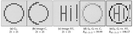
Figure 6. R evaluation depends on mistake distances but depends on an area contained in a window around a mistake point. $I_R$ corresponds to the value of $R_W$ for each pixel. Images representing $I_R$ in (d,e) correspond to inverse images. Here, the window size around each mistake is of size $W=3\times 3$.

2.2.3. The Failure Measure $FM$

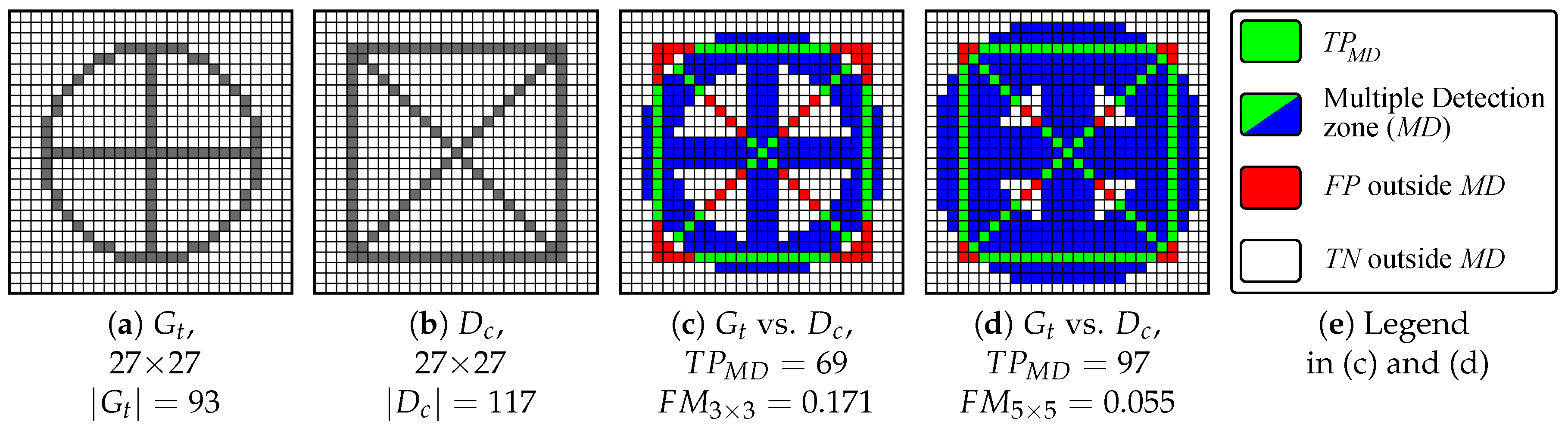
The $failure$ $measure$ [46] is an extension of [20] (see beginning of Section 2). These evaluation computes four criteria, taking into account a multiple detection zone ($MD$). The detection zone of the ideal image can be represented as a dilation of $G_t$, creating a rough edge, as illustrated in Figure 7. Then, the criteria are as follows: (1) False negative ($F{N}_{FM}$), (2) False positive ($F{P}_{FM}$), (3) Multiple detection ($D{M}_{FM}$) and (4) Localization ($LO{C}_{FM}$). They are computed by:

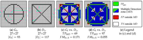
Figure 7. Failure Measure ($FM$) evaluation with two different Multiple Detection ($MD$) zones: in (c), dilation of $G_t$ with structuring element 3 × 3, and 5 × 5 in (d). The greater the $MD$ area, the lower the $FM$ error.

• $F{N}_{FM}={\displaystyle \frac{max(0,|G_t|-T{P}_{MD})}{|G_t|}}$, where $T{P}_{MD}$ represents the number of points of $D_c$ in $MD$ (see Figure 7 and Figure 8), green pixels,
  

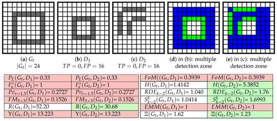  Figure 8. Different $D_c$: number of false positive points ($FP$) and false negative points ($FN$) are the same for $D_1$ and for $D_2$ but the distances of FNs and the shapes of the two $D_c$ are different. The legend for (d,e) is available in Figure 7.
• $F{P}_{FM}={\displaystyle \frac{F{P}_{MD}}{|I|-|MD|}}$, with $F{P}_{MD}$ the number of points of $D_c$ outside $MD$ and $|MD|$ denoting the number of pixels of $MD$, see Figure 7 and Figure 8, green and blue pixels,
• $D{M}_{FM}={\displaystyle \frac{T{P}_{MD}-TP}{|MD|-|G_t|}}$, $TP$ representing the number of TPs (see above),
• $LO{C}_{FM}={\displaystyle \frac{1}{|G_t|·\mathcal{C}}}·{\sum }_{p\in G_t}max(\mathcal{C},d(p,D_c))$, where $\mathcal{C}$ is a constant ($\mathcal{C}=5$ in our experiments) and $d(p,D_c)$ represents the Euclidean distance between p and $D_c$ (see next section). In [20], $LO{C}_{FM}$ represents the number of rows containing a point around the vertical edge.

On end, the $failure$ $measure$ ($FM$) is defined as:

$$FM(G_t,D_c)=\alpha ·F{N}_{FM}+\beta ·F{P}_{FM}+\gamma ·D{M}_{FM}+\delta ·LO{C}_{FM},$$

(5)

with ($\alpha ,\beta ,\gamma ,\delta$) four positive coefficients such that $\alpha +\beta +\gamma +\delta =1$; in the experiments: $\alpha =0.4,\beta =0.4,\gamma =0.1$ and $\delta =0.1$. Unfortunately, due to the multiple detection zone, $FM$ behaves like $Pv$ for the evaluation of small object segmentation, as shown in Figure 8, and $FM$ obtains the same measurement for two different shapes.

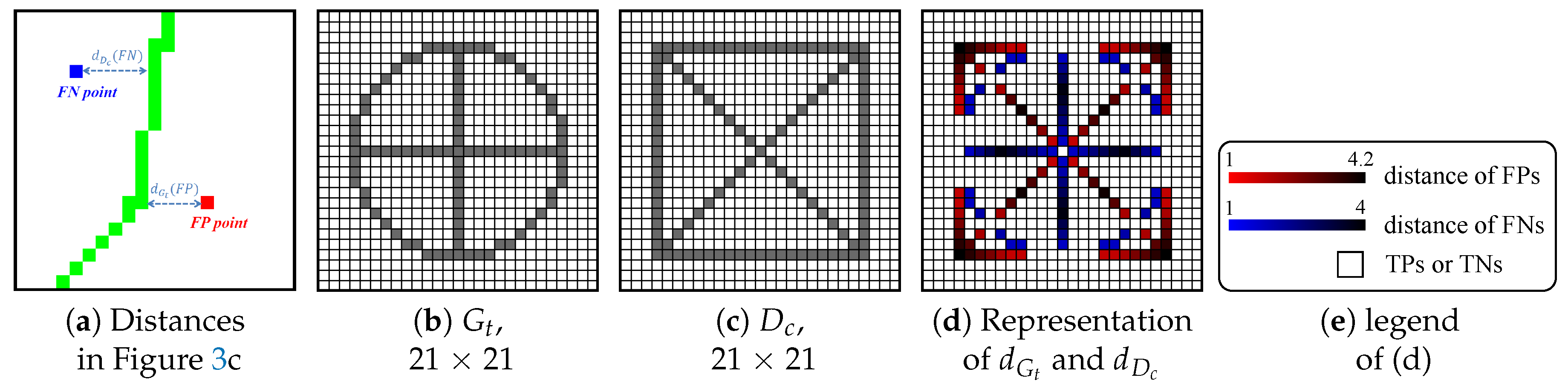
2.3. Assessment Involving Distances of Misplaced Pixels

A reference-based edge map quality measure requires that a displaced edge should be penalized in function not only of FPs and/or FNs, but also of the distance from the position where it should be located. Table 4 reviews the most relevant measures involving distances. Thus, for a pixel p belonging to the desired contour $D_c$, $d_{G_t}\left(p\right)$ represents the minimal Euclidian distance between p and $G_t$. If p belongs to the ground truth $G_t$, $d_{D_c}\left(p\right)$ is the minimal distance between p and $D_c$, and Figure 9a shows the difference between $d_{G_t}\left(p\right)$ and $d_{D_c}\left(p\right)$. Mathematically, denoting $(x_p,y_p)$ and $(x_t,y_t),$ the pixel coordinates of two points p and t, respectively; thus, $d_{G_t}\left(p\right)$ and $d_{D_c}\left(p\right)$ are described by:

$$\left\{\begin{array}{cc}\mathrm{for}p\in D_c:& \\ d_{G_t}\left(p\right)& =\mathrm{Inf}\left\{\sqrt{{(x_p-x_t)}^2+{(y_p-y_t)}^2},t\in G_t\right\},\\ \mathrm{for}p\in G_t:& \\ d_{D_c}\left(p\right)& =\mathrm{Inf}\left\{\sqrt{{(x_p-x_t)}^2+{(y_p-y_t)}^2},t\in D_c\right\}.\end{array}\right.$$

Table 4. List of error measures involving distances, generally: $k=1$ or $k=2$ , and, $\kappa =0.1$ or $\kappa =1/9$ .

Error Measure Name	Formulation	Parameters
Pratt’s Figure of Merit (FoM) [47]	${\displaystyle FoM\left(G_t,D_c\right)=1-{\displaystyle \frac{1}{\max \left(\left|G_t\right|,\left|D_c\right|\right)}}·{\displaystyle \sum _{p\in D_c}}\frac{1}{1+\kappa ·d_{G_t}^2\left(p\right)}}$	$\kappa \in \left]0;1\right]$
$FoM$ revisited [48]	$F\left(G_t,D_c\right)=1-\frac{1}{\left|G_t\right|+\beta ·FP}·{\displaystyle {\displaystyle \sum _{p\in G_t}}\frac{1}{1+\kappa ·d_{D_c}^2\left(p\right)}}$	$\kappa \in \left]0;1\right]$ and $\beta \in {\mathbb{R}}^{+}$
Combination of $FoM$ and statistics [49]	$d_4\left(G_t,D_c\right)=\frac{1}{2}·\sqrt{{\displaystyle {\displaystyle \frac{{\left(TP-\max \left(\left|G_t\right|,\left|D_c\right|\right)\right)}^2+F{N}^2+F{P}^2}{{\left(\max \left(\left|G_t\right|,\left|D_c\right|\right)\right)}^2}}}+Fo{M}^2\left(G_t,D_c\right)}$	$\kappa \in \left]0;1\right]$ and $\beta \in {\mathbb{R}}^{+}$
Edge map quality measure [50]	$D_p\left(G_t,D_c\right)=\frac{1/2}{\left|I\right|-\left|G_t\right|}·{\displaystyle {\displaystyle \sum _{p\in FP}}\left(1-\frac{1}{1+\kappa ·d_{G_t}^2\left(p\right)}\right)}+\frac{1/2}{\left|G_t\right|}·{\displaystyle {\displaystyle \sum _{p\in FN}}\left(1-\frac{1}{1+\kappa ·d_{TP}^2\left(p\right)}\right)}$	$\kappa \in \left]0;1\right]$
Symmetric FoM [21]	$SFoM\left(G_t,D_c\right)=\frac{1}{2}·FoM\left(G_t,D_c\right)+\frac{1}{2}·FoM\left(D_c,G_t\right)$	$\kappa \in \left]0;1\right]$
Maximum FoM [21]	$MFoM\left(G_t,D_c\right)=max\left(FoM\left(G_t,D_c\right),FoM\left(D_c,G_t\right)\right)$	$\kappa \in \left]0;1\right]$
Yasnoff measure [51]	$\mathsf{{\rm Y}}\left(G_t,D_c\right)=\frac{100}{\left|I\right|}·\sqrt{{\displaystyle \sum _{p\in D_c}}{d}_{G_t}^2\left(p\right)}$	None
Hausdorff distance [52]	$H\left(G_t,D_c\right)=max\left({\displaystyle {\displaystyle \underset{p\in D_c}{max}}\left(d_{G_t}\left(p\right)\right),{\displaystyle {\displaystyle \underset{p\in G_t}{max}}}\left(d_{D_c}\left(p\right)\right)}\right)$	None
Maximum distance [24]	${\displaystyle f_2{d}_6\left(G_t,D_c\right)=max\left(\frac{1}{\left|D_c\right|}·{\displaystyle \sum _{p\in D_c}}{d}_{G_t}\left(p\right),\frac{1}{\left|G_t\right|}·{\displaystyle \sum _{p\in G_t}}{d}_{D_c}\left(p\right)\right)}$	None
Distance to $G_t$ [24,26,53]	$D^k\left(G_t,D_c\right)={\displaystyle \frac{1}{\left|D_c\right|}}·\sqrt[k]{{\displaystyle \sum _{p\in D_c}}{d}_{G_t}^k\left(p\right)}$, $k=1$ for [24,53]	$k\in {\mathbb{R}}^{+}$
Oversegmentation [54]	$\mathsf{\Theta }\left(G_t,D_c\right)=\frac{1}{FP}·{\displaystyle \sum _{p\in D_c}}{\left(\frac{d_{G_t}\left(p\right)}{{\delta }_{TH}}\right)}^k$	for [54]: $k\in {\mathbb{R}}^{+}$ and ${\delta }_{TH}\in {{\mathbb{R}}_{\ast }}^{+}$
Under-segmentation [54]	$\mathsf{\Omega }\left(G_t,D_c\right)=\frac{1}{FN}·{\displaystyle \sum _{p\in G_t}}{\left(\frac{d_{D_c}\left(p\right)}{{\delta }_{TH}}\right)}^k$	for [54]: $k\in {\mathbb{R}}^{+}$ and ${\delta }_{TH}\in {{\mathbb{R}}_{\ast }}^{+}$
$Relative$ $Distance$ $Error$ [24,55,56]	$RD{E}_k\left(G_t,D_c\right)=\sqrt[k]{{\displaystyle \frac{1}{\left|D_c\right|}}·{\displaystyle \sum _{p\in D_c}}{d}_{G_t}^k\left(p\right)}+\sqrt[k]{{\displaystyle \frac{1}{\left|G_t\right|}}·{\displaystyle \sum _{p\in G_t}}{d}_{D_c}^k\left(p\right)}$,	$k\in {\mathbb{R}}^{+}$, $k=1$ for [24], $k=2$ for [55,56]
Symmetric distance [24,26]	${\displaystyle S^k\left(G_t,D_c\right)=\sqrt[k]{\frac{{\displaystyle \sum _{p\in D_c}}{d}_{G_t}^k\left(p)\right)+{\displaystyle \sum _{p\in G_t}}{d}_{D_c}^k\left(p\right)}{\left|D_c\cup G_t\right|}}}$,    $k=1$ for [24]	$k\in {\mathbb{R}}^{+}$
Baddeley’s Delta Metric [57]	${\Delta }^k(G_t,D_c)=\sqrt[k]{\frac{1}{|I|}·{\displaystyle \sum _{p\in I}}{|w\left(d_{G_t}\left(p\right)\right)-w\left(d_{D_c}\left(p\right)\right)|}^k}$	$k\in {\mathbb{R}}^{+}$ and a convex function $w:\mathbb{R}\mapsto \mathbb{R}$
Magnier et al. measure [58]	$\mathsf{\Gamma }(G_t,D_c)=\frac{FP+FN}{|G_t{|}^2}·\sqrt{{\displaystyle \sum _{p\in D_c}}{d}_{G_t}^2\left(p\right)}$	None
Complete distance measure [21]	$\mathsf{\Psi }(G_t,D_c)=\frac{FP+FN}{|G_t{|}^2}·\sqrt{{\displaystyle \sum _{p\in G_t}}{d}_{D_c}^2\left(p\right)+{\displaystyle \sum _{p\in D_c}}{d}_{G_t}^2\left(p\right)}$	None
$\lambda$ measure [59]	$\lambda (G_t,D_c)=\frac{FP+FN}{|G_t{|}^2}·\sqrt{{\displaystyle \sum _{p\in D_c}}{d}_{G_t}^2\left(p\right)+min\left(|G_t{|}^2,\frac{|G_t{|}^2}{T{P}^2}\right)·{\displaystyle \sum _{p\in G_t}}{d}_{D_c}^2\left(p\right)}$	None

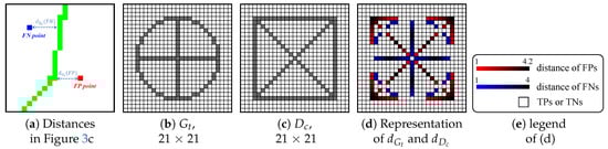
Figure 9. Example of ground truth ($G_t$) versus (vs.) a desired contour ($D_c$).

These distance functions refer to the Euclidean distance. Figure 9d illustrates an example of $d_{G_t}\left(p\right)$ and $d_{D_c}\left(p\right)$.

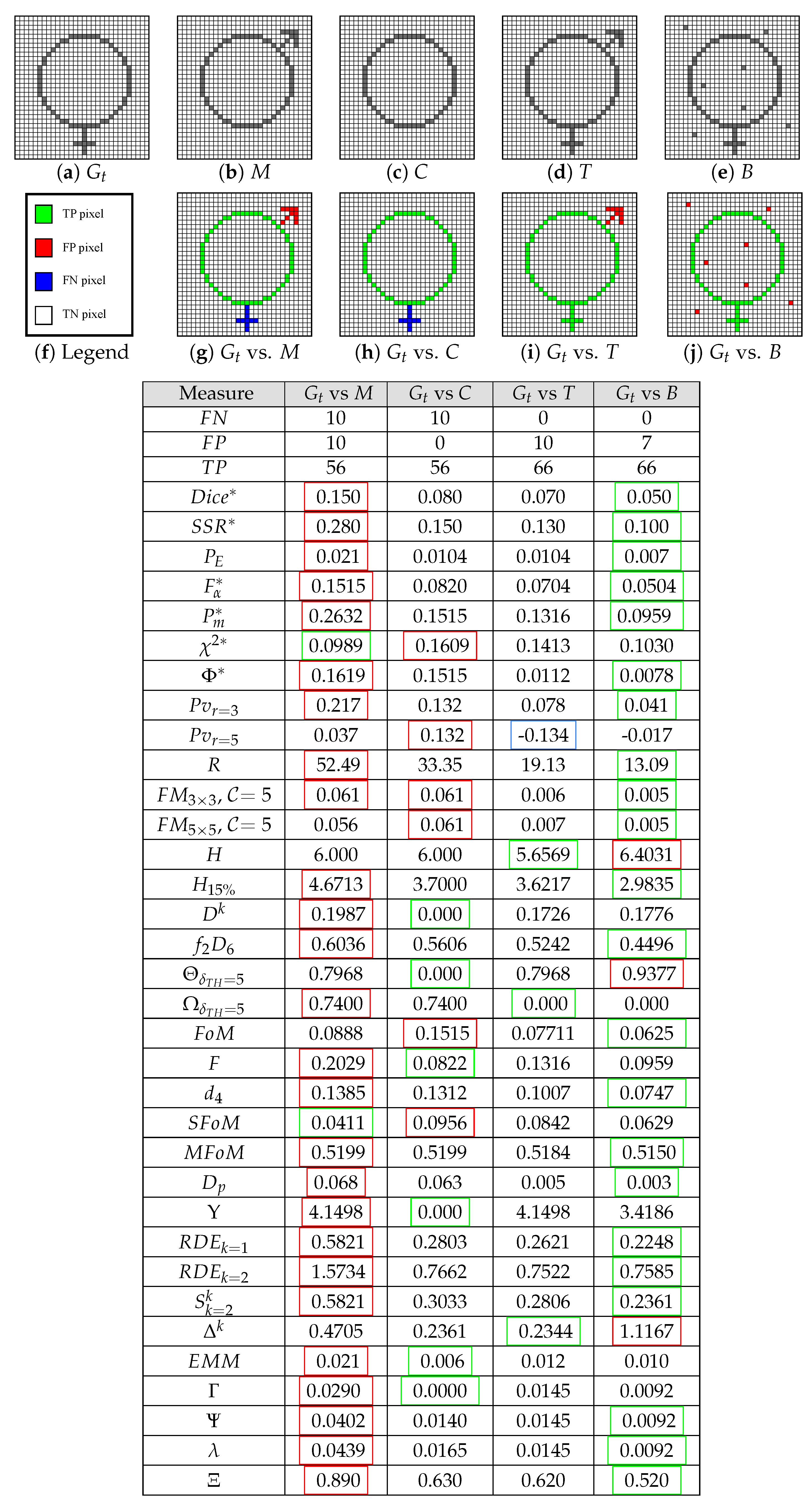
On the one hand, some distance measures are specified in the evaluation of over-segmentation (i.e., presence of FPs), for example: $\mathsf{{\rm Y}}$, $D^k$, $\mathsf{\Theta }$ and $\mathsf{\Gamma }$; others are presented and detailed in [21,24]. On the other hand, the $\mathsf{\Omega }$ measure assesses an edge detection by computing only under-segmentation (FNs). Other edge detection evaluation measures consider both distances of FPs and FNs [14]. A perfect segmentation using an over-segmentation measure could be an image including no edge points and an image having the most undesirable edge points (FPs) concerning under-segmentation evaluations [60], as shown in Figure 10 and Figure 11. In addition, another limitation of only over- and under-segmentation evaluations are that several binary images can produce the same result (Figure 8). Therefore, as demonstrated in [14], a complete and optimum edge detection evaluation measure should combine assessments of both over- and under-segmentation, as $f_2{d}_6$, $S^k$, $RD{E}_k$, $\mathsf{\Psi }$ and $\lambda$, illustrated in Figure 8.

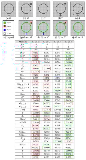
Figure 10. Evaluation measure results for different $D_c$ images in (b–e) using the same $G_t$ in (a).

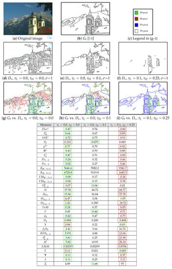
Figure 11. Evaluation measure results for a real image segmented [4] at different hysteresis thresholds.

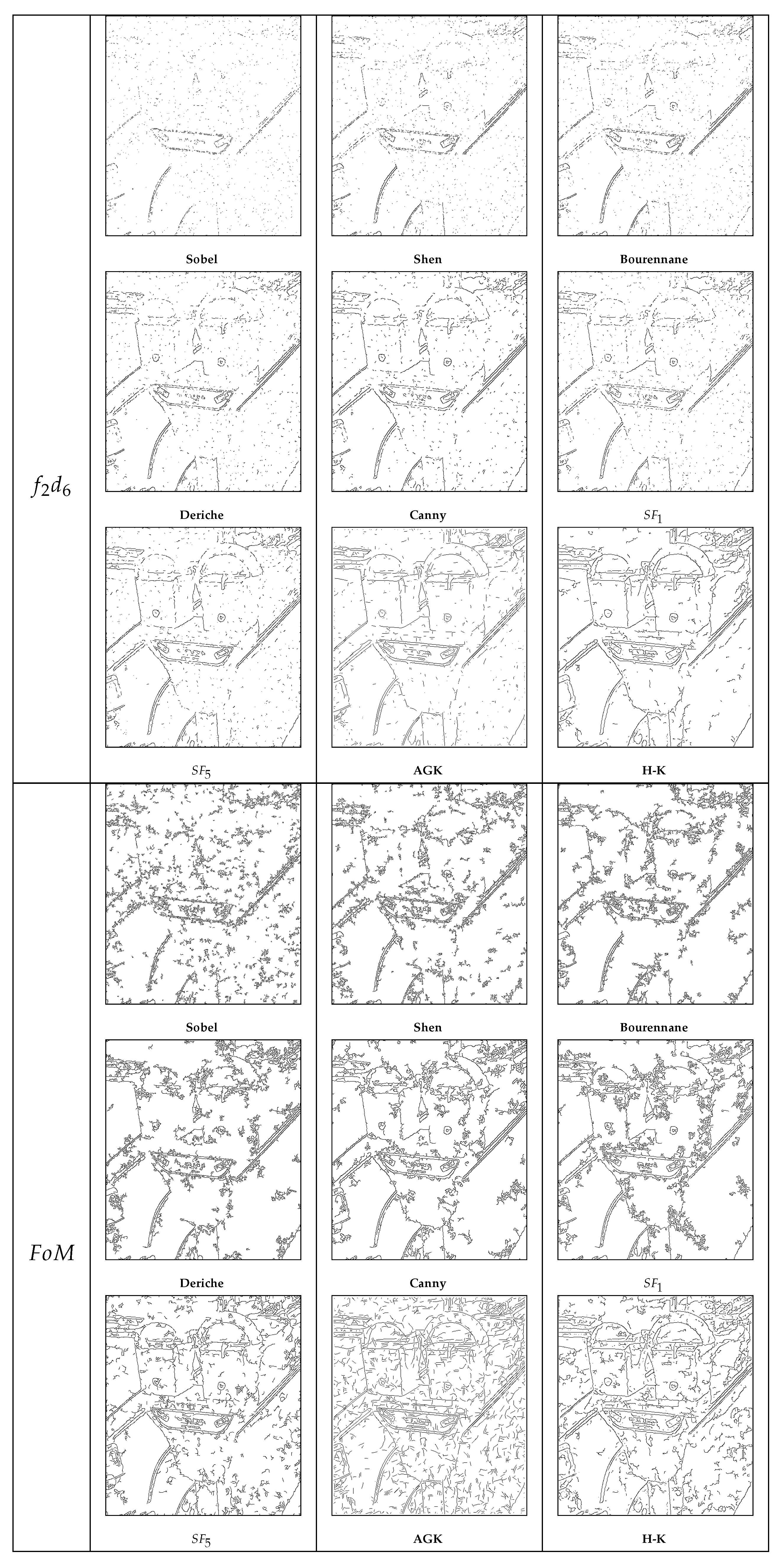
Among the distance measures between two contours, one of the most popular descriptors is named the Figure of Merit ($FoM$). This distance measure has an advantage because it ranges from 0 to 1, where 0 corresponds to a perfect segmentation [47]. Nonetheless, for $FoM$, the distance of the FNs is not recorded and are strongly penalized as statistic measures:

$$\begin{array}{cc}FoM\left(G_t,D_c\right)& ={\displaystyle 1-{\displaystyle \frac{1}{\max \left(\left|G_t\right|,\left|D_c\right|\right)}}·{\displaystyle \sum _{p\in TP}}\frac{1}{1+\kappa ·d_{G_t}^2\left(p\right)}-{\displaystyle \frac{1}{\max \left(\left|G_t\right|,\left|D_c\right|\right)}}·{\displaystyle \sum _{p\in FP}}\frac{1}{1+\kappa ·d_{G_t}^2\left(p\right)}}\hfill \\ & ={\displaystyle 1-{\displaystyle \frac{TP}{\max \left(\left|G_t\right|,\left|D_c\right|\right)}}-{\displaystyle \frac{1}{\max \left(\left|G_t\right|,\left|D_c\right|\right)}}·{\displaystyle \sum _{p\in FP}}\frac{1}{1+\kappa ·d_{G_t}^2\left(p\right)}.}\hfill \end{array}$$

For example, in Figure 10, $FoM(G_t,C)>FoM(G_t,M)$, whereas M contains both FPs and FNs and C only FNs. Furthermore, for the extreme cases, knowing that $TP=|G_t|-FN$, the $FoM$ measures takes the following values:

• if $FP=0$: $FoM\left(G_t,D_c\right)=1-{\displaystyle \frac{TP}{|G_t|}}=1-{\displaystyle \frac{|G_t|-FN}{|G_t|}}$,
• if $FN=0$: $FoM\left(G_t,D_c\right)=1-\frac{TP}{\left|D_c\right|}-\frac{1}{\left|D_c\right|}·{\sum }_{p\in FP}\frac{1}{1+\kappa ·d_{G_t}^2\left(p\right)}$.

When $FN$>0 and $FP$ are constant, it behaves like matrix-based error assessments (Figure 10). Moreover, for $FP$>0, the $FoM$ penalizes over-detection very lightly compared to under-detection. Several evaluation measures are derived from $FoM$: F, $d_4$, $D_p$, $MFoM$ and $SFoM$. Contrary to $FoM$, the F measure computes the distances of FNs but not of the FPs, so F behaves inversely to $FoM$, it can be rewritten as:

$$\begin{array}{cc}F\left(G_t,D_c\right)& =1-\frac{1}{\left|G_t\right|+\beta ·FP}·{\displaystyle {\displaystyle \sum _{p\in TP}}\frac{1}{1+\kappa ·d_{D_c}^2\left(p\right)}}-\frac{1}{\left|G_t\right|+\beta ·FP}·{\displaystyle {\displaystyle \sum _{p\in FN}}\frac{1}{1+\kappa ·d_{D_c}^2\left(p\right)}}\hfill \\ & =1-\frac{TP}{\left|G_t\right|+\beta ·FP}-\frac{1}{\left|G_t\right|+\beta ·FP}·{\displaystyle {\displaystyle \sum _{p\in FN}}\frac{1}{1+\kappa ·d_{D_c}^2\left(p\right)}}.\hfill \end{array}$$

Therefore, for the extreme cases, the F measures takes the following values:

• if $FP=0$: $F\left(G_t,D_c\right)=1-\frac{TP}{\left|G_t\right|}-\frac{1}{\left|G_t\right|}·{\displaystyle {\displaystyle \sum _{p\in FN}}\frac{1}{1+\kappa ·d_{D_c}^2\left(p\right)}}$,
• if $FN=0$: $F\left(G_t,D_c\right)=1-\frac{TP}{\left|G_t\right|+\beta ·FP}$.

In addition, the $d_4$ measure depends particularly on $TP$, $FP$, $FN$ and ≈1/4 on $FoM$, but $d_4$ penalizes FNs like the $FoM$ measure; it is a close idea to the $FM$ measure (Section 2.2). Otherwise, $SFoM$ and $MFoM$ take into account both distances of FNs and FPs, so they can compute a global evaluation of a contour image. However, $MFoM$ does not consider FPs and FNs at the same time, contrary to $SFoM$. Another way to compute a global measure is presented in [50] with the edge map quality measure $D_p$. The right term computes the distances of the FNs between the closest correctly detected edge pixel, i.e., $G_t\cap D_c$, $D_p$ can be rewritten as:

$$D_p(G_t,D_c){\displaystyle \frac{{\displaystyle FP-{\displaystyle \sum _{p\in FP}}\frac{1}{1+\kappa ·d_{G_t}^2\left(p\right)}}}{2·\left|I\right|-2·\left|G_t\right|}}+{\displaystyle \frac{{\displaystyle FN-{\displaystyle \sum _{p\in FN}}\frac{1}{1+\kappa ·d_{G_t}^2\left(p\right)}}}{2·\left|G_t\right|}}.$$

Finally, $D_p$ is more sensitive to FNs than FPs because of the huge coefficient $\frac{1}{|I|-|G_t|}$.

A second measure widely computed in matching techniques is represented by the Hausdorff distance H, which measures the mismatch of two sets of points [52]. This measure is useful in object recognition, the algorithm aims to minimize H, which measures the mismatch of two shapes [61,62]. This max-min distance could be strongly deviated by only one pixel that can be positioned sufficiently far from the pattern (Figure 10). There are several enhancements of the Hausdorff distance presented in [24,63,64]. Furthermore, $f_2{d}_6$ and $D^k$ are often called “Modified Hausdorff Distance” (abbreviated $MHD$) in the literature. As another example, one idea to improve the measure is to compute H with a proportion of the maximum distances; let us note $H_{5\%}$—this measure for 5% of the values [52]. Nevertheless, as pointed out in [24], an average distance from the edge pixels in the candidate image to those in the ground truth is more appropriate, like $S^k$, $RD{E}_k$ or $\mathsf{\Psi }$. Thus, the score of the $f_2{d}_6$ corresponds to the maximum between the over- and the under-segmentation (depending on $\frac{1}{|D_c|}$ and $\frac{1}{|G_t|}$, respectively), whereas the values obtained by $S^k$ represents their mean. Moreover, $S^k$ takes small values in the presence of low level of outliers, whereas the score becomes large as the level of mistaken points increases [24,26] but is sensitive to remote misplaced points as presented in [21]. On the other hand, the Relative Distance Error ($RD{E}_k$) computes both the over- and the under-segmentation errors separately, with the weights $\frac{1}{|D_c|}$ and $\frac{1}{|G_t|}$, respectively. Otherwise, derived from H, the Delta Metric (${\Delta }^k$) [57] intends to estimate the dissimilarity between each element of two binary images, but is highly sensitive to distances of misplaced points [14,21]. All of these edge detection evaluation measures are reviewed in [21] with their advantages and disadvantages (excepted $RD{E}_k$), and, as concluded in [21,25], a complete and optimum edge detection evaluation measure should combine assessments of both over- and under-segmentation, as $f_2{d}_6$, $S^k$, $H_{15\%}$, $RD{E}_k$ and $\mathsf{\Psi }$.

On another note, the Edge Mismatch Measure ($EMM$) depending on TPs and both $d_{D_c}$ and $d_{G_t}$. In [36], this measure is combined with others (including $ME$ and $D^k$) in order to compare several thresholding methods. Indeed, ${\delta }_{D_c/G_t}\left(p\right)$ is a threshold distance function penalizing high distances (exceeding a value $M_{dist}$) and $EMM$ is represented as follows:

$${\displaystyle EMM(G_t,D_c)=1-\frac{TP}{TP+\omega \left[{\sum }_{p\in FN}{\delta }_{D_c}\left(p\right)+ϵ·{\sum }_{p\in FP}{\delta }_{G_t}\left(p\right)\right]}}$$

(6)

with ${\delta }_{D_c}$ and ${\delta }_{G_t}$ two cost functions of $d_{D_c}$ and $d_{G_t}$ respectively discarding/penalizing outliers [36]:

$${\delta }_{D_c}\left(p\right)=\left\{\begin{array}{cc}{d}_{D_c}\left(p\right),\hfill & \mathrm{if}{d}_{D_c}\left(p\right)<M_{dist}\hfill \\ D_{max},\hfill & \mathrm{otherwise},\hfill \end{array}\right.\mathrm{and}{\delta }_{G_t}\left(p\right)=\left\{\begin{array}{cc}{d}_{G_t}\left(p\right),\hfill & \mathrm{if}{d}_{G_t}\left(p\right)<M_{dist}\hfill \\ D_{max},\hfill & \mathrm{otherwise}.\hfill \end{array}\right.$$

(7)

Thus, $\omega$ is the penalty weighting distance measures ${\delta }_{D_c}$ and ${\delta }_{G_t}$, whereas $ϵ$ represents a weight for distances of FPs only. For this purpose, the set of parameters are suggested as follows:

• $M_{dist}=0.025·|I|$,
• $D_{max}={\displaystyle \frac{|I|}{10}}$,
• $\omega ={\displaystyle \frac{10}{|I|}}$,
• $ϵ=2$.

Note that the suggested parameters depend on $|I|$, the total number of pixels in I. Moreover, $EMM$ computes a score different from 1 if there exists at least one TP (cf. Figure 8). Finally, when the $EMM$ score is close to 0, the segmentation is qualified as acceptable, whereas a score close to 1 corresponds to a poor edge detection.

3. A New Objective Edge Detection Assessment Measure

3.1. Influence of the Penalization of False Negative Points in Edge Detection Evaluation

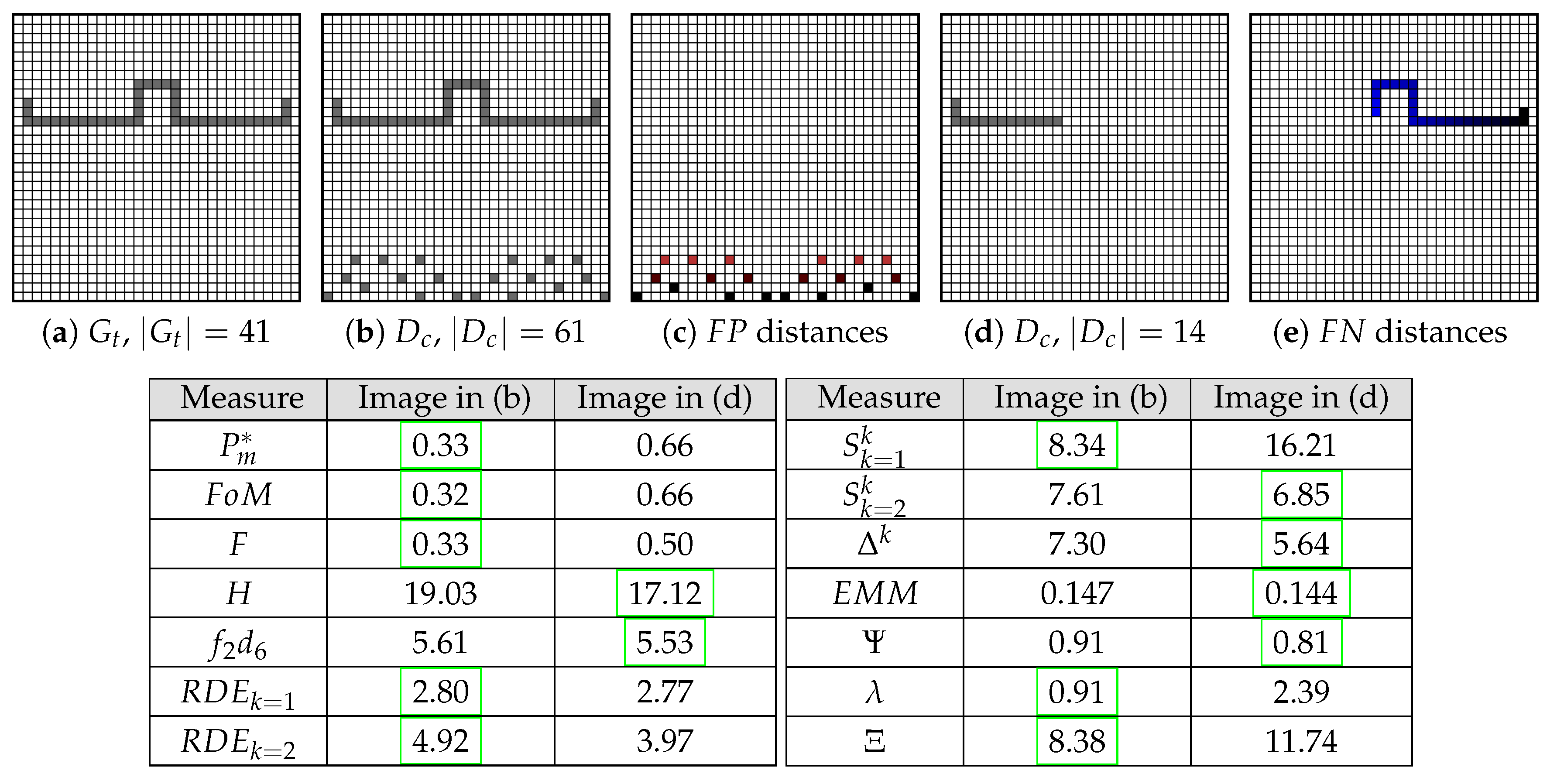
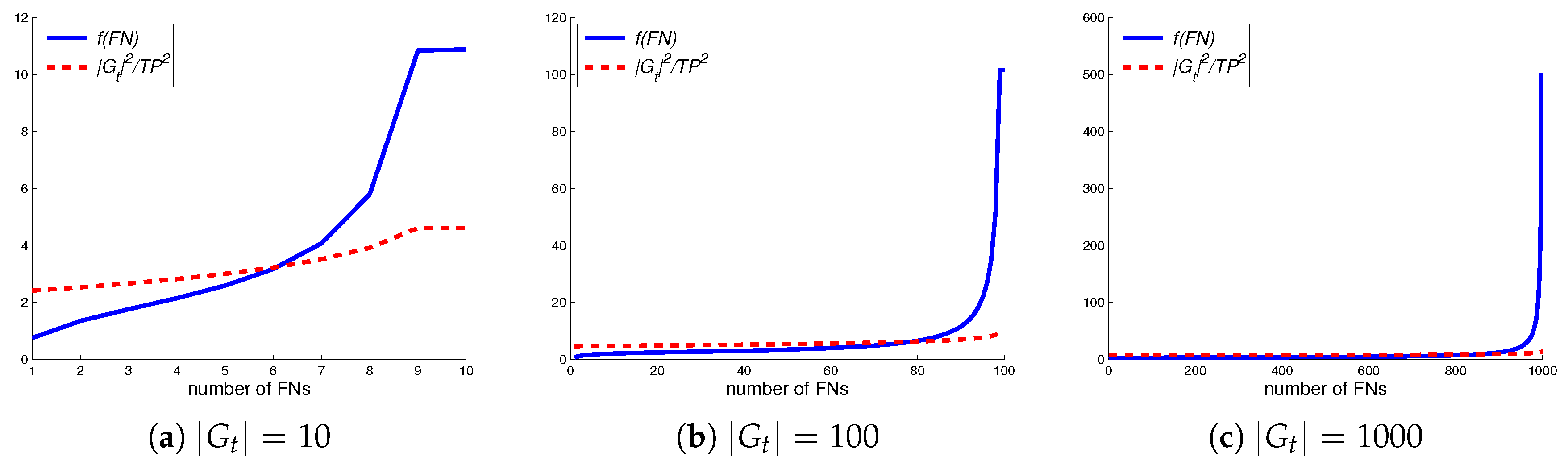
Several edge detection measures have been presented above. Clearly, taking into account both FP and FN distances is more objective for the assessment. However, there are two main problems concerning the edge detection measures involving distances. First, a single (or a few) FP point(s) at a sufficiently high distance may penalize a good detection (see Figure 12c). This is a well known problem concerning the Hausdorff distance. Thus, best scores for each measure obtained in an objective way (cf. next section) are not necessarily tied to the most efficient detector. Secondly, the edge maps associated with these scores lack many desired contours, because distances of FPs strongly penalize edge detectors evaluated by the majority of these measures. On the contrary, distances of FN points are neither recorded (as over-segmentation measures), nor penalized enough (cf. Figure 12b). In other words, FNs are, generally, as penalized as FPs. Moreover, FNs are often close to detected edges (TPs or FPs close to $G_t$), most error measures involving distances do not consider this particularity because ${\sum }_{p\in FN}{d}_{D_c}$ are less important than ${\sum }_{p\in FP}{d}_{G_t}$. Note that $RD{E}_k$ computes ${\sum }_{p\in FN}{d}_{D_c}$ and ${\sum }_{p\in FP}{d}_{G_t}$ separately. In [59], a measure of the edge detection assessment is developed: it is denoted $\lambda$ and improves the segmentation measure $\mathsf{\Psi }$ (see formulas in Table 4). The $\lambda$ measure penalizes highly FNs compared to FPs (as a function of their mistake distances), depending on the number of TPs. Typically, contours of desired objects are in the middle of the image, but rarely on the periphery. Thus, using or $f_2{d}_6$, $S^k$, ${\Delta }^k$, or $\mathsf{\Psi }$, a missing edge in the image remains insufficiently penalized contrary to the distance of FPs, which could be too high, as presented in Figure 13, contrary to $\lambda$. Another example, in Figure 10, $\mathsf{\Psi }(G_t,C)<\mathsf{\Psi }(G_t,T)$, whereas C should be more penalized because of FNs that do not enable the object to be identified. The more FNs are present in $D_c$, the more $D_c$ must be penalized as a function of $d_{G_t}$, because the desirable object becomes unrecognizable, as $D_c$ in Figure 11c. In addition, $D_c$ should be penalized as a function of $d_{G_t}$, of the $FN$ number, as stated above. For $\lambda$, the term influencing the penalization of FN distances can be rewritten as: $\frac{|G_t{|}^2}{T{P}^2}={\left(\frac{FN+TP}{TP}\right)}^2={\left(1+\frac{FN}{TP}\right)}^2⩾1$, ensuring a stronger penalty for $d_{G_t}^2$, compared to $d_{D_c}^2$. The min function avoids the multiplication by infinity when $TP=0$. When $|G_t|=TP$, $\lambda$ is equivalent to $\mathsf{\Psi }$ and $\mathsf{\Gamma }$ (see Figure 10, image T). In addition, compared to $\mathsf{\Psi }$, $\lambda$ penalizes more $D_c$ having FNs, than $D_c$ with only FPs, as illustrated in Figure 10 (images C and T). Finally, the weight $\frac{|G_t{|}^2}{T{P}^2}$ tunes the $\lambda$ measure by considering an edge map of better quality when FNs points are localized close to the desired contours $D_c$, the red dot curve in Figure 14 represents this weight function. Hence, the $\lambda$ function is able to assess images that are not too large, as in Figure 10, Figure 12 and Figure 13; however, the penalization is not enough for larger images. Indeed, the main difficulty remains the $FN+FP$ coefficient to the left of $\lambda$; as a result, the image in Figure 11a is considered by this measure as the best one. The solution is to separate the two entities $FN$ and $FP$ and insert them directly inside the root square of the measure, firstly to modulate the FPs distances and secondly to weight the FN distances. Therefore, the new edge evaluation assessment formula is given by:

$$\mathsf{\Xi }(G_t,D_c)=\frac{1}{|G_t|}·\sqrt{\left(FP·{\displaystyle \sum _{p\in D_c}}{d}_{G_t}^2\left(p\right)+f\left(FN\right)·{\displaystyle \sum _{p\in G_t}}{d}_{D_c}^2\left(p\right)\right)}$$

(8)

with

$$f\left(TP\right)=\left\{\begin{array}{cc}log\left(FN\right)·e^{FN},\hfill & \mathrm{if}TP=0,\mathrm{i}.\mathrm{e}.,|G_t|=FN\hfill \\ log\left(FN+1\right)·e^{\frac{|G_t|}{TP}},\hfill & \mathrm{elsewhere}.\hfill \end{array}\right.$$

(9)

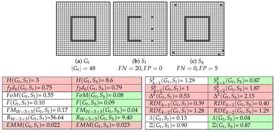
Figure 12. A single (or a few) FP point(s) at a sufficiently high distance may penalize a good detection. $S_b$ represents $G_t$ in (a) with only five FPs that penalize the shape using several edge detection evaluation functions.

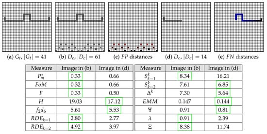
Figure 13. Edge detection evaluations must be more sensitive to $FN$ distances than $FP$ distances. In (b), $|D_c|=61$, so there are 20 FPs, whereas, in (d), $|D_c|=14$, so there are 27 FNs; so $FP<FN$.

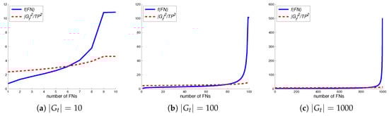
Figure 14. Several examples of f function evolution as a function of the FN number.

The f function influencing the penalization of FN distances ensures a strong penalty for $d_{D_c}^2$, compared to $d_{G_t}^2$ (see blue curves in Figure 14). There exist several f functions than may effectively accomplish the purpose. When $FN=0$, $f\left(TP\right)=0$, and only the FP distances are recorded, pondered by the number of FPs. Otherwise, if $TP=0$, so $|G_t|=FN$, thus $f\left(TP\right)=log\left(FN\right)·e^{FN}$ to avoid a division by 0, and $log\left(FN\right)·e^{FN}>log\left(FN+1\right)·e^{\frac{|G_t|}{TP}}$. Finally, by separating the two weights for $d_{D_c}^2$ and $d_{G_t}^2$ penalizes $D_c$ images containing FPs and/or $D_c$ images with missing edges (FNs).

The next subsection details the way to evaluate an edge detector in an objective way. Results presented in this paper show the importance to penalize false negative points more severely than false positive points because the desired objects are not always completely visible using ill-suited evaluation measure, and $\mathsf{\Xi }$ provides a reliable edge detection assessment.

3.2. Minimum of the Measure and Ground Truth Edge Image

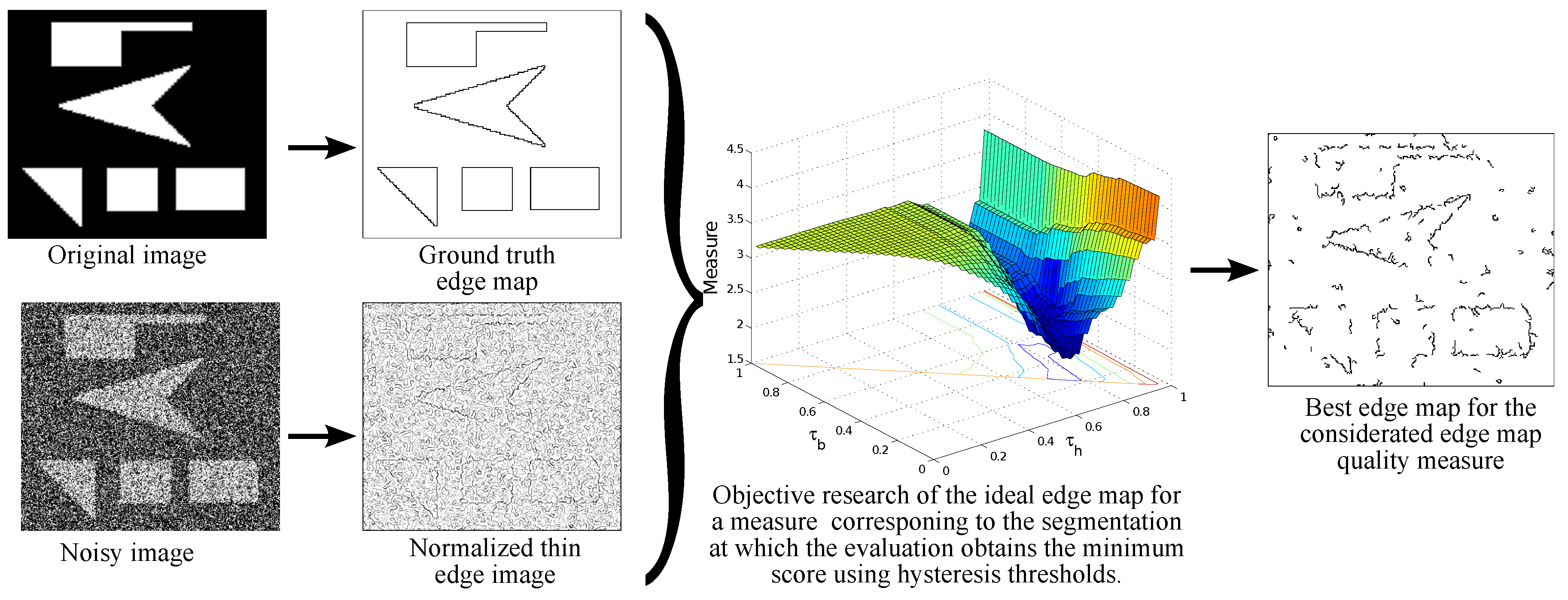
Dissimilarity measures are used to assess the divergence of binary images. Instead of manually choosing a threshold to obtain a binary image (see Figure 3 in [14]), the purpose is to compute the minimal value of a dissimilarity measure by varying the thresholds (double loop: loop over ${\tau }_L$ and loop over ${\tau }_H$) of the thin edges obtained by filtering gradient computations (see Table 1). Compared to a ground truth contour map, the ideal edge map for a measure corresponds to the desired contour at which the evaluation obtains the minimum score for the considered measure among the thresholded (binary) images. Theoretically, this score corresponds to the thresholds at which the edge detection represents the best edge map, compared to the ground truth contour map [14,25,46]. Figure 15 illustrates the choice of a contour map as a function of ${\tau }_L$ and ${\tau }_H$. Algorithm 1 represents this argmin function and summarizes the different steps to compute an ideal edge map concerning a chosen measure.

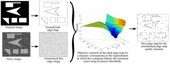
Figure 15. Example of computation of a minimum score for a given measure.

Algorithm 1 Calculates the minimum score and the best edge map of a given measure $Meas$

Require:  $|\nabla I|$        : normalized thin gradient image Require:  $G_t$           : Ground Truth edge image Require: $Hyster$   : hysteresis threshold function Require: $Meas$      : Measure computing a dissimilarity score between $G_t$ and a desired contour $D_c$   $ste{p}_{\tau }=0.01$               % step for the loops on thresholds    $scor{e}_L=realmax$    % the largest finite floating-point number     for ${\tau }_H=0:ste{p}_{\tau }:1$ do     for ${\tau }_L=0:ste{p}_{\tau }:1$ do       if ${\tau }_H⩾{\tau }_L$ then         $D_c\leftarrow Hyster(|\nabla I|,{\tau }_L,{\tau }_H)$         $score\leftarrow Meas(G_t,D_c)$         if $scor{e}_L⩾score$ then           $scor{e}_L\leftarrow scor{e}_L$    % ideal score             $Idea{l}_{D_c}\leftarrow D_c$          % ideal edge map         end if        end if      end for    end for

Since low thresholds lead to heavy over-segmentation and high thresholds may create numerous false-negative pixels, the minimum score of an edge detection evaluation should be a compromise between under- and over-segmentation (detailed and illustrated in [14]).

As demonstrated in [14], the significance of the choice of ground truth map influences the dissimilarity evaluations. Indeed, if not reliable [43], a ground truth contour map that is inaccurate in terms of localization penalizes precise edge detectors and/or advantages the rough algorithms as edge maps presented in [13,15]. For these reasons, the ground truth edge map concerning the real image in our experiments is built semi-automatically, as detailed in [14].

4. Experimental Results

The aim of the experiments is to obtain the best edge map in a supervised way. The importance of an assessment penalizing false negative points more severely compared to false positive points has been shown above. In order to study the performance of the edge detection evaluation measures, the hysteresis thresholds vary and the minimum score of the studied measure corresponds to the best edge map (cf. Figure 15). The thin edges of real noisy images are computed by nine filtering edge detectors:

• Sobel [3],
• Shen [5],
• Bourennane [7],
• Deriche [6],
• Canny [4],
• Steerable filter of order 1 ($S{F}_1$) [9],
• Steerable filter of order 5 ($S{F}_5$) [10],
• Anisotropic Gaussian Kernels (AGK) [11,65,66],
• Half Gaussian Kernels (H-K) [12,56].

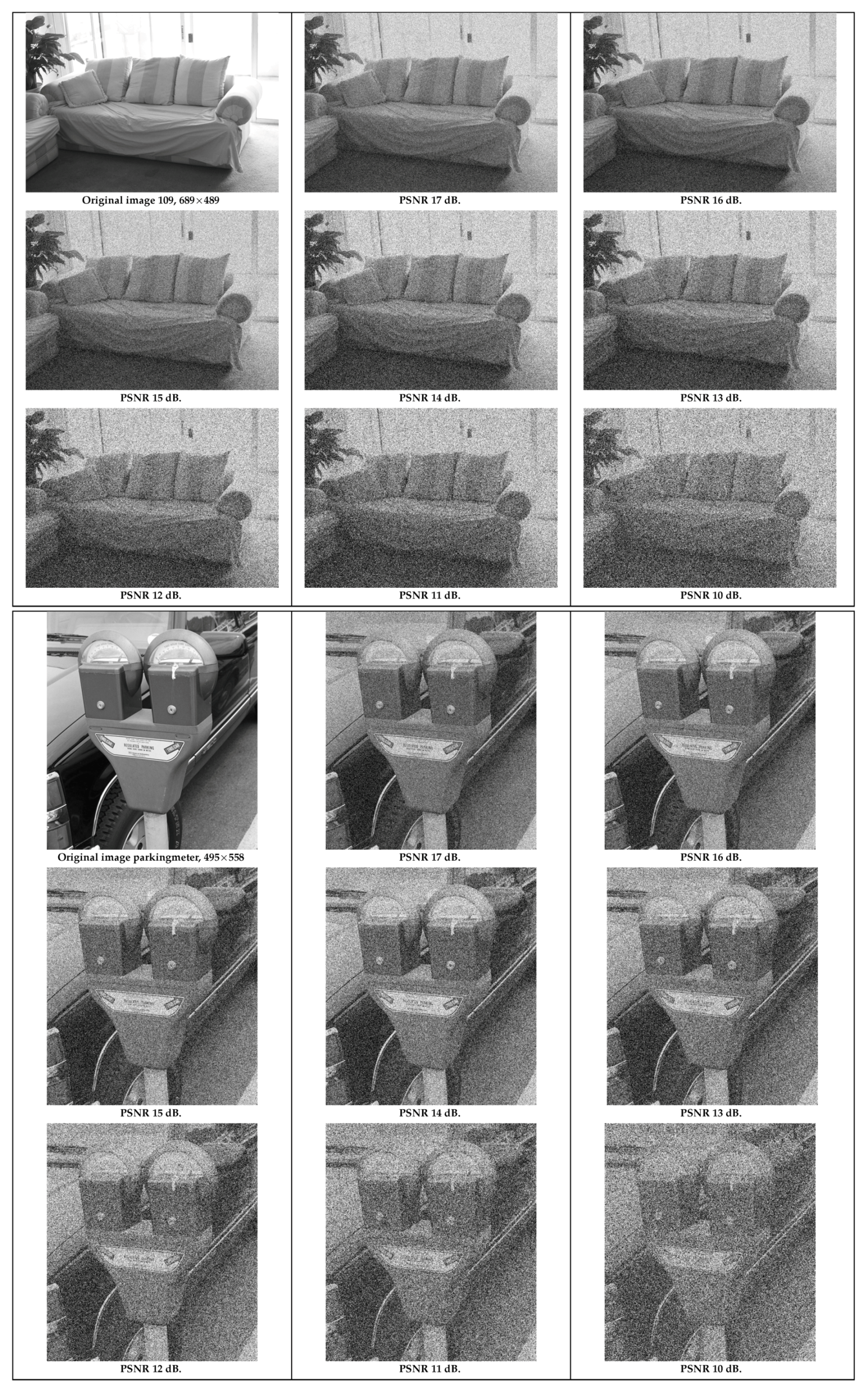
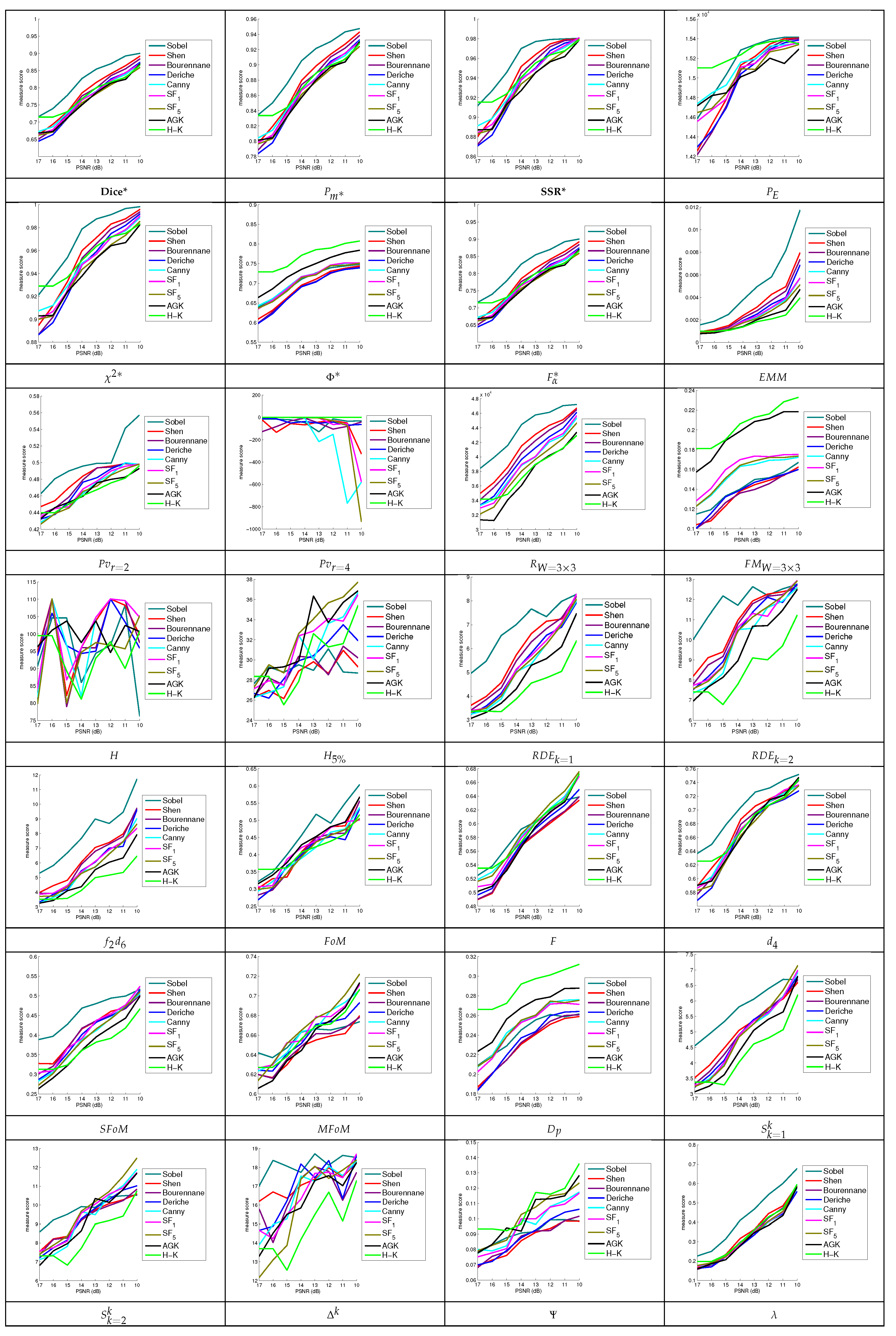
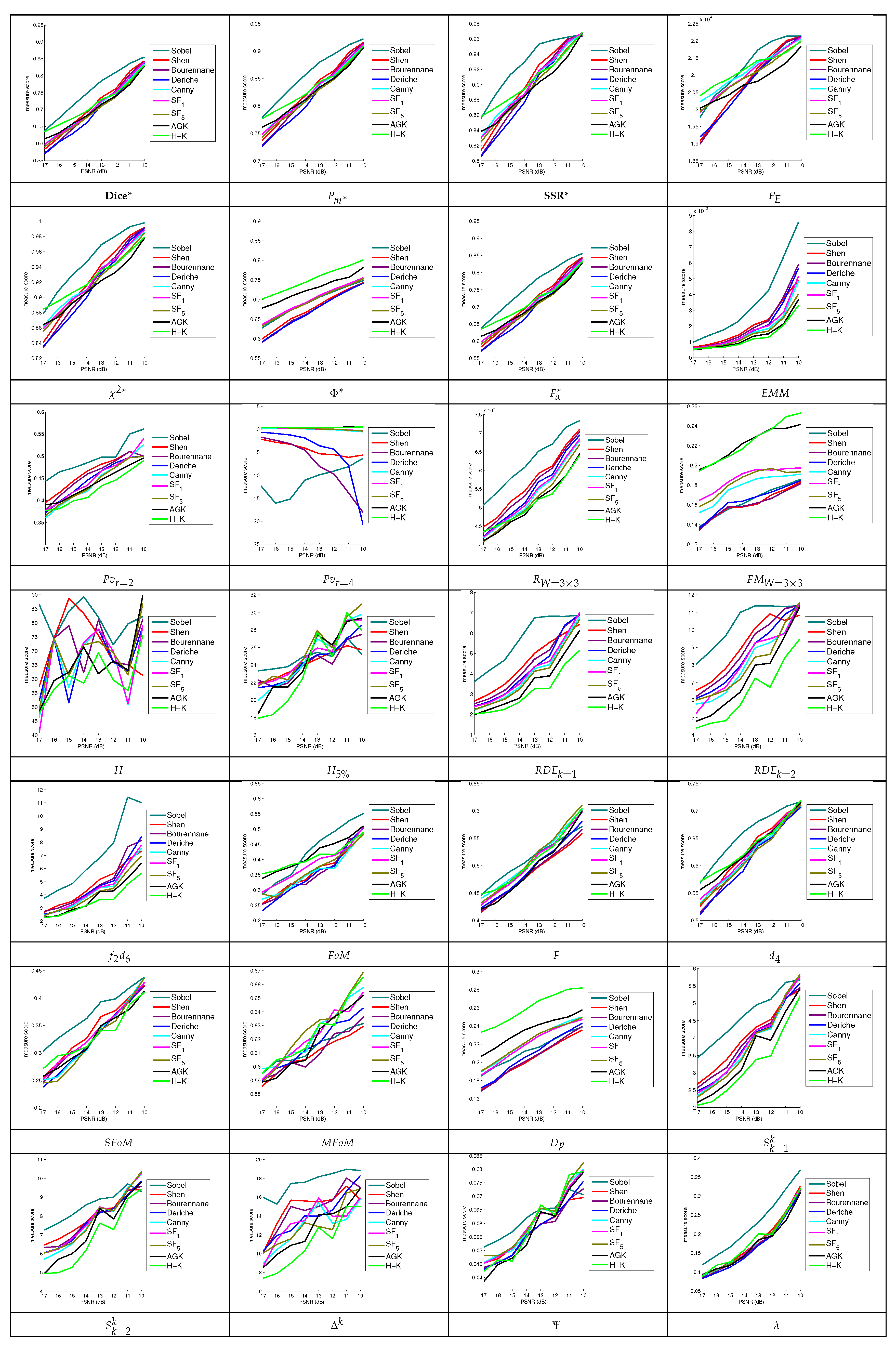
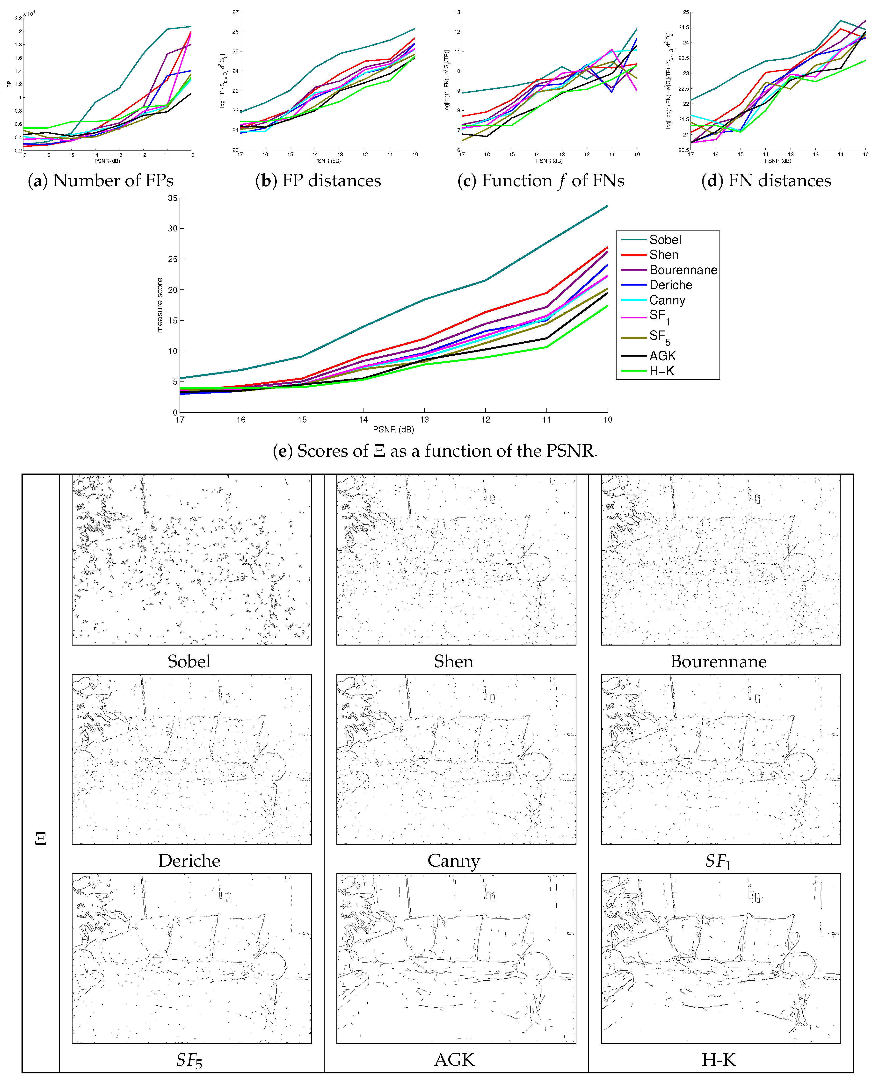
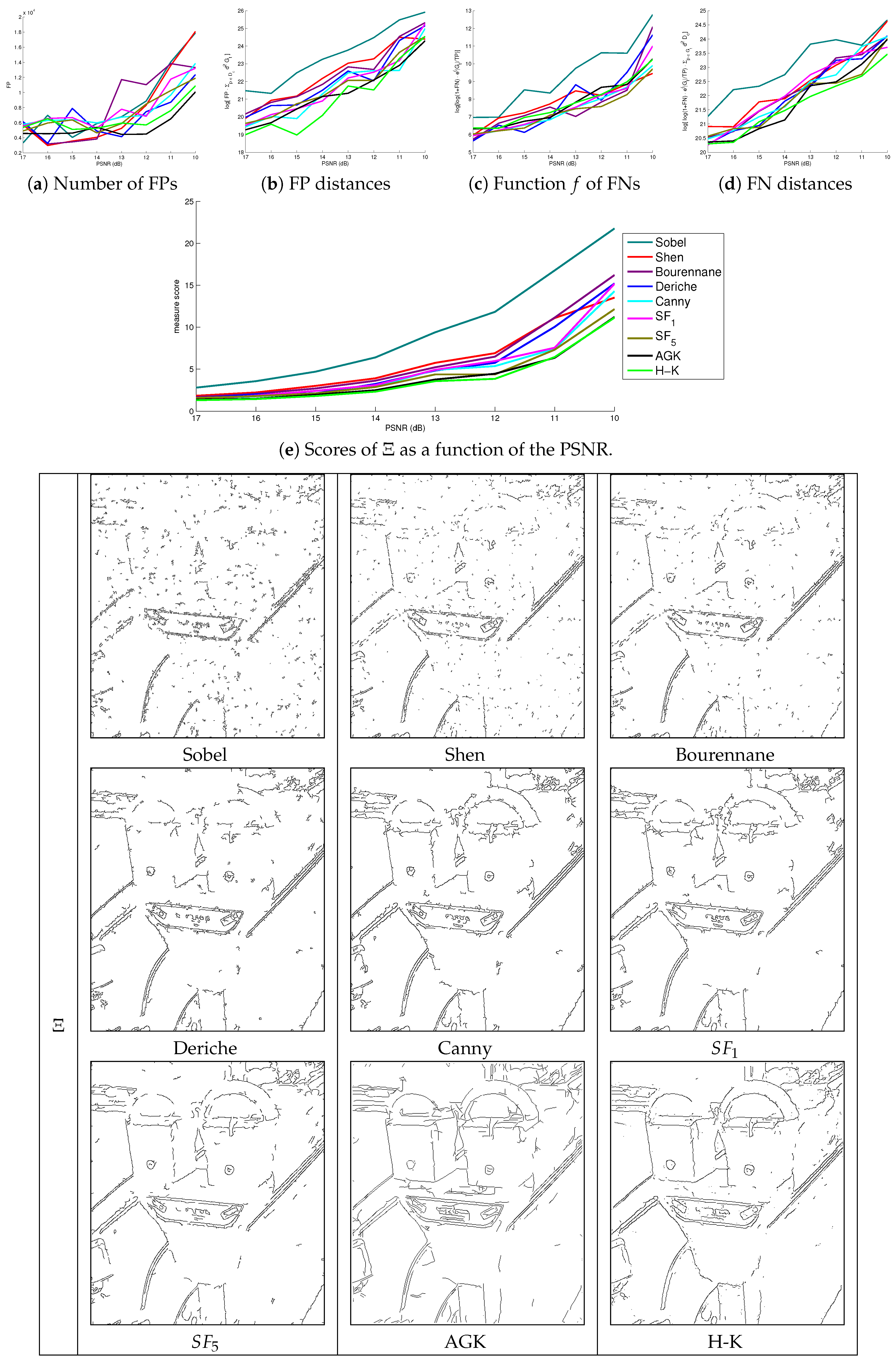
The kernels of these methods are size-adaptable, except for the Sobel operator that corresponds to a 3 × 3 mask. The parameters of the filters are chosen to keep the same spatial support for the derivative information, e.g., $\sigma =1.5$ for Gaussians (details of these filters are available in [56]). Ground truth images ($G_t$) are shown in Figure 16, whereas corrupted and original images are presented in Figure 17. The scores of the different measures are recorded by varying the thresholds of the normalized thin edges computed by an edge detector and plotted as a function of the noise level in the original image, as presented in Figure 18 and Figure 19. A plotted curve should increase monotonously with noise level (Gaussian noise), represented by Peak Signal to Noise Ratio (PSNR) values (from 17 dB to 10 dB). Among all the edge detectors, box (Sobel [3]) and exponential (Shen [5], Bourennane [7] filters do not delocalize contour points [67], whereas they are sensitive to noise (i.e., addition of FPs). The Deriche [6] and Gaussian filters [4] are less sensitive to noise, but suffer from rounding corners and junctions (see [67,68]) as the oriented filters $S{F}_1$ [9], $S{F}_5$ [10] and AGK [11], but the more the 2D filter is elongated, the more the segmentation remains robust against noise. Finally, as a compromise, H-K correctly detects contour points that have corners and is robust against noise [12]. Consequently, the scores of the evaluation measures for the first three filters must be lower than the three last ones, and, Canny, Deriche and $S{F}_1$ scores must be situated between these two sets of assessments. Furthermore, as $S{F}_5$, AGK and H-K are less sensitive to noise than other filters, the ideal segmented image for these three algorithms should be visually closer to $G_t$. The presented segmentations correspond to the original image for a PSNR = 14 dB. Therefore, on the one hand, considered segmentations must be tied to the robustness of the detector. On the other hand, the scores must increase monotonously, with an increasing order as a function of the edge detector quality. Note that the matlab code of $FoM$, $D^k$, $S^k$ and ${\Delta }^k$ measures are available at http://kermitimagetoolkit.net/library/code/. The matlab code of several other measures are available on MathWorks: https://fr.mathworks.com/matlabcentral/fileexchange/63326-objective-supervised-edge-detection-evaluation-by-varying-thresholds-of-the-thin-edges.

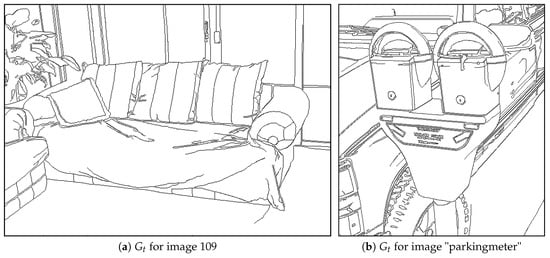
Figure 16. Ground truth edge images tied to original images available in Figure 17 used in the presented experiments. These $G_t$ images are available in [14].

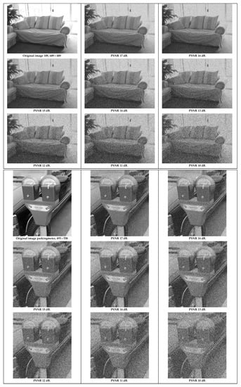
Figure 17. Image 109 (top) and image “parkingmeter” (bottom) at different levels of noise (PSNR).

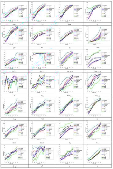
Figure 18. Image 109: Comparison of edge detection evaluation evolution as a function of PSNR values.

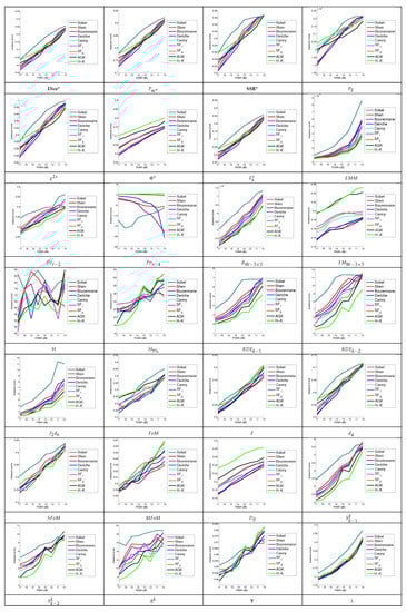
Figure 19. Image parkingmeter: Comparison of edge detection evaluation evolutions.

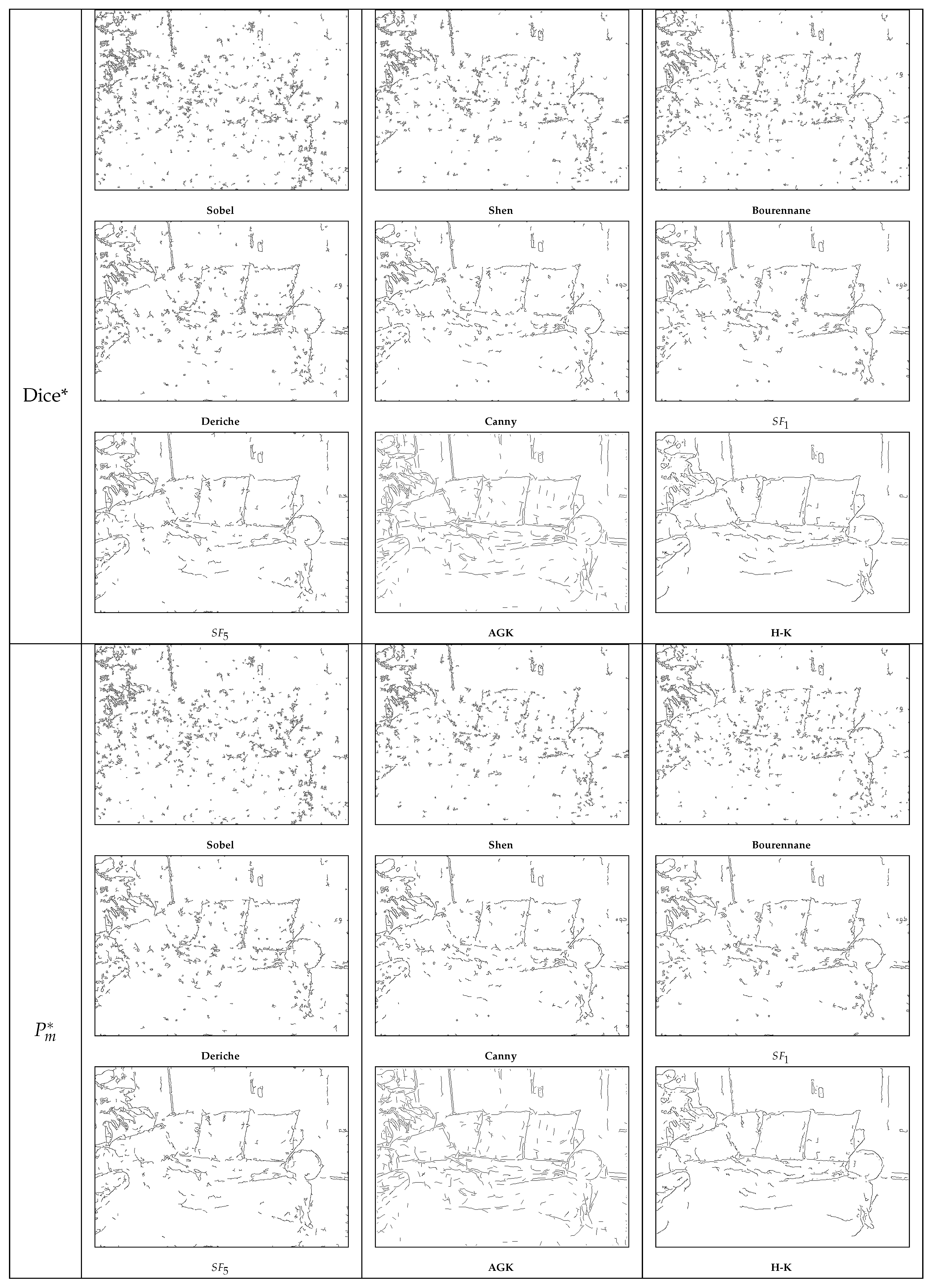
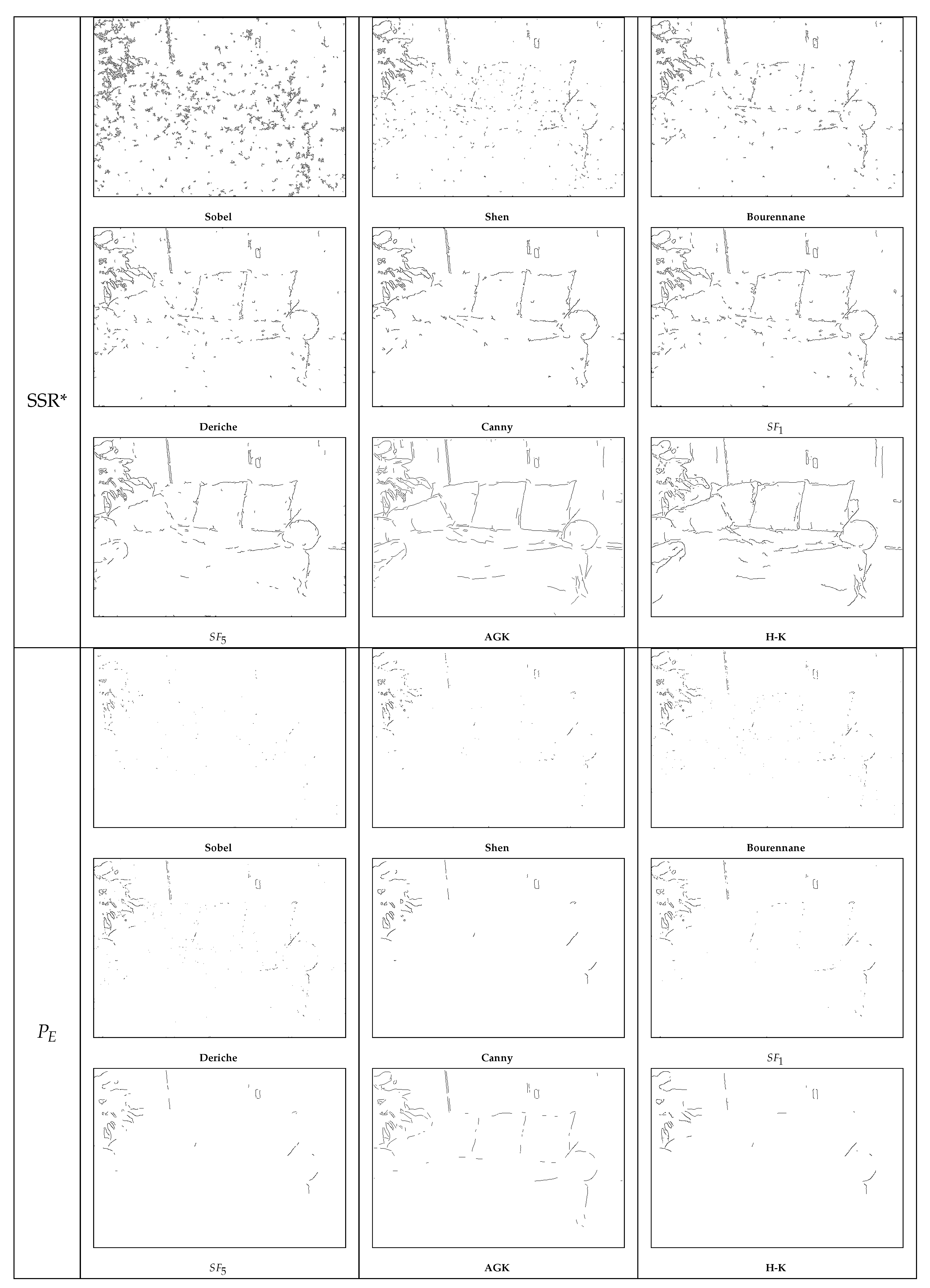
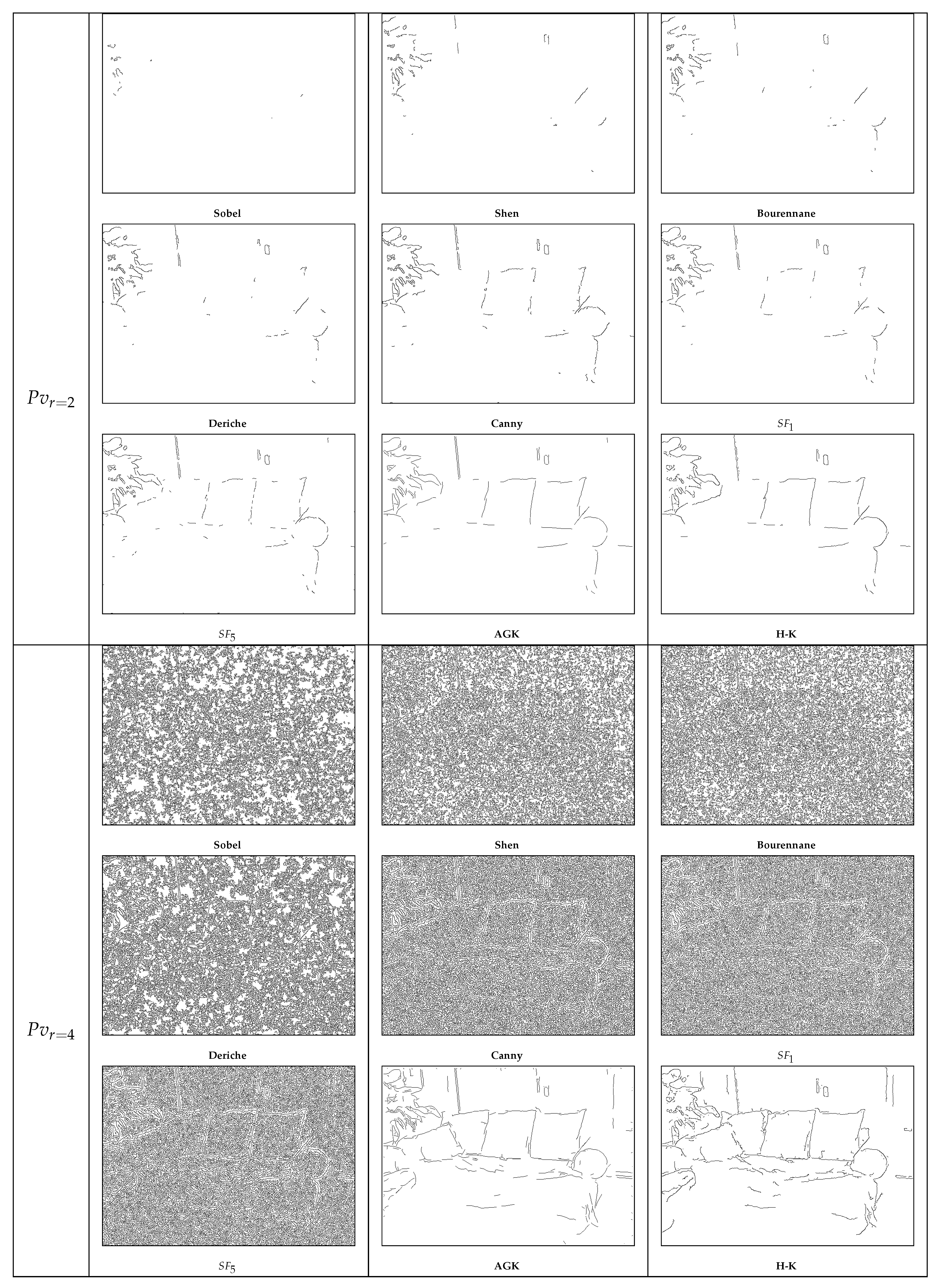
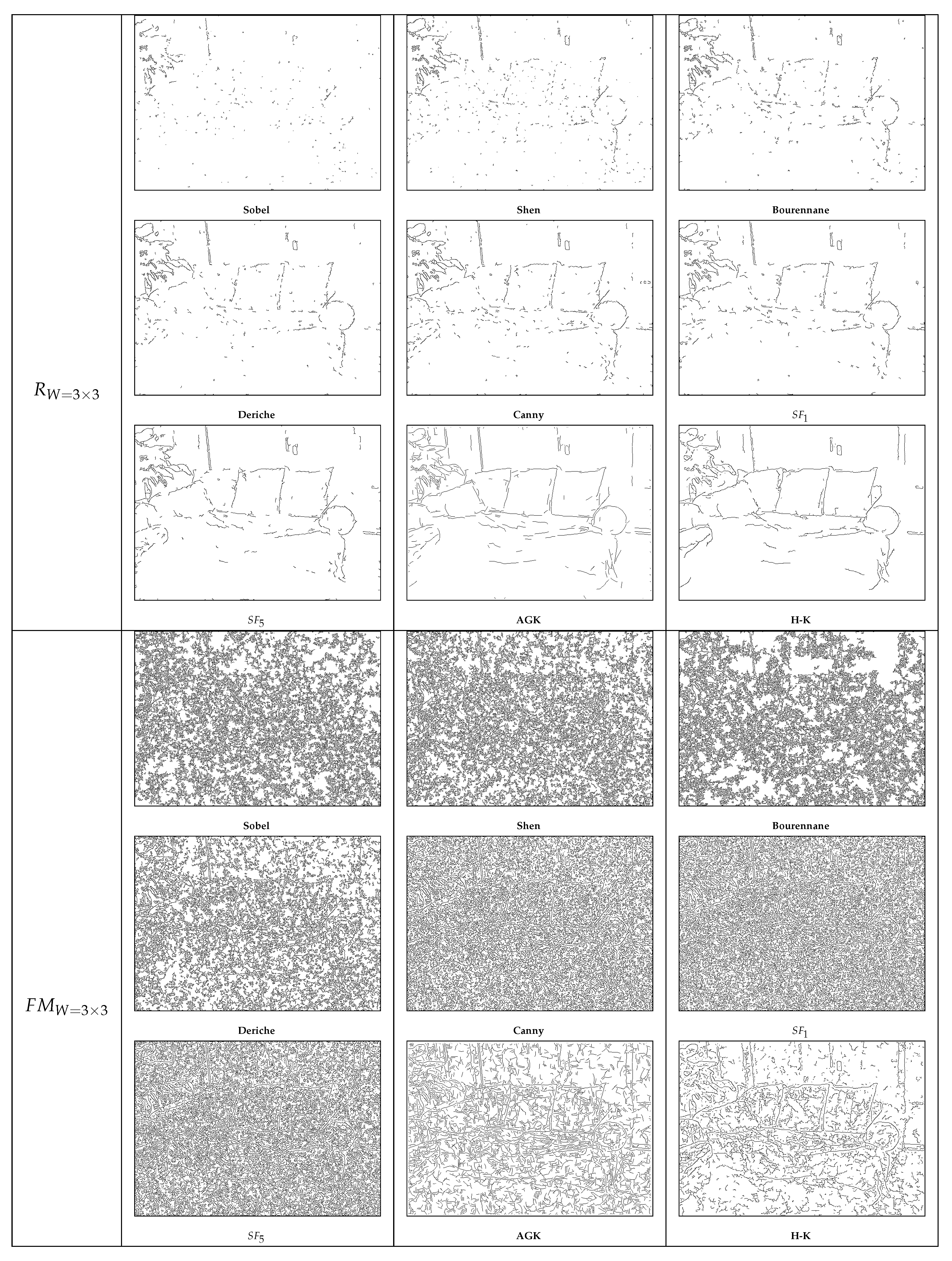
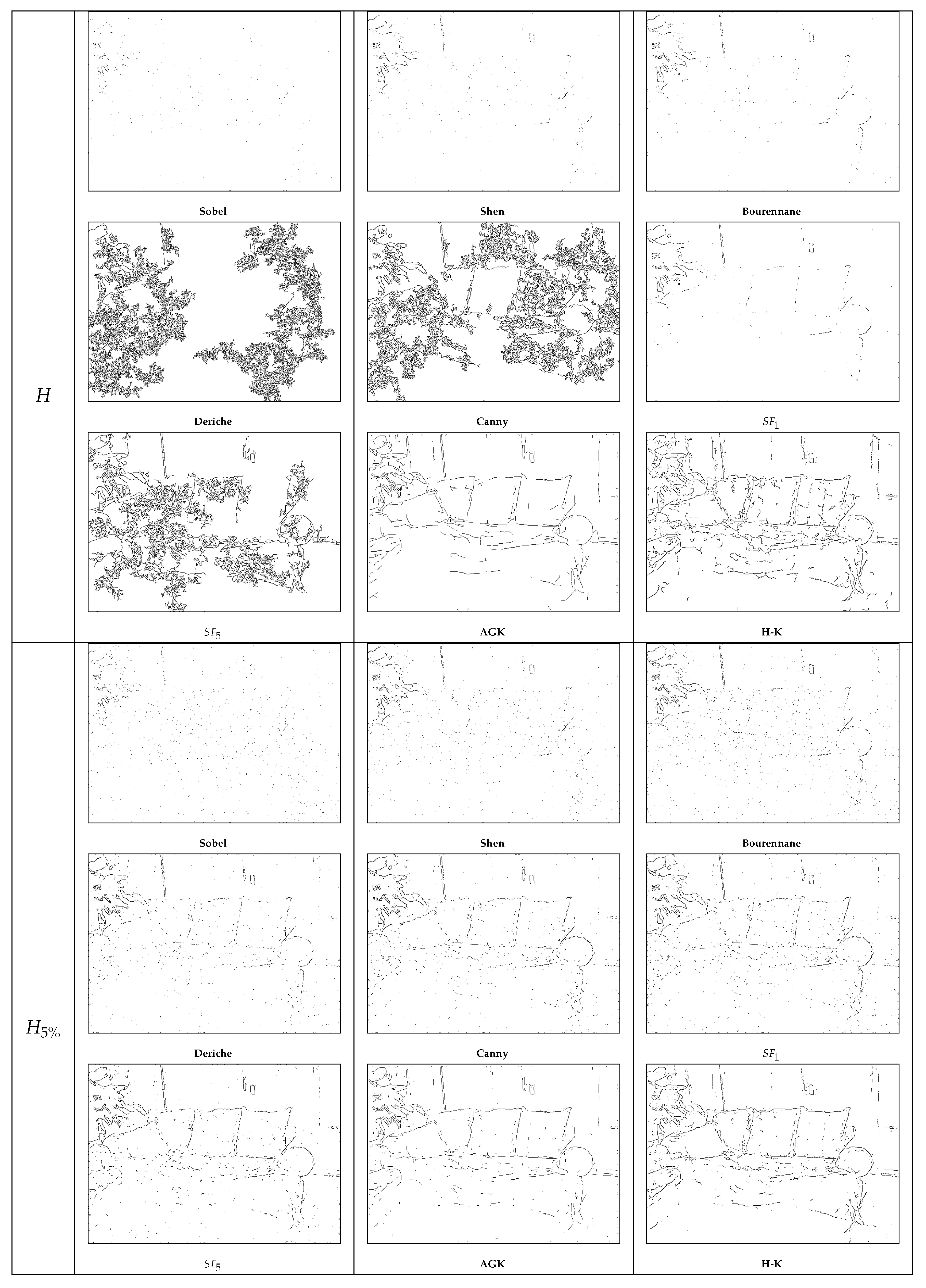
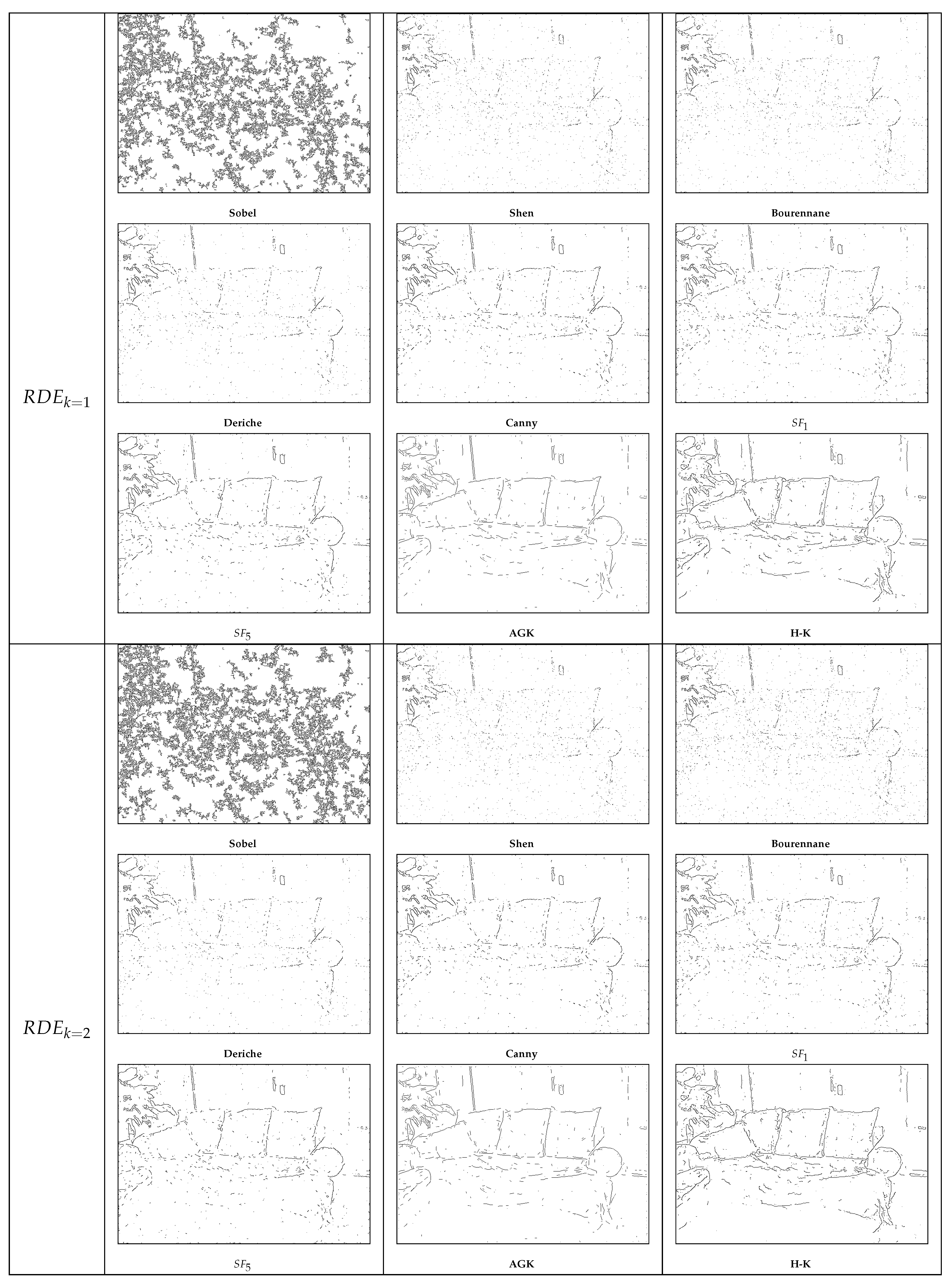
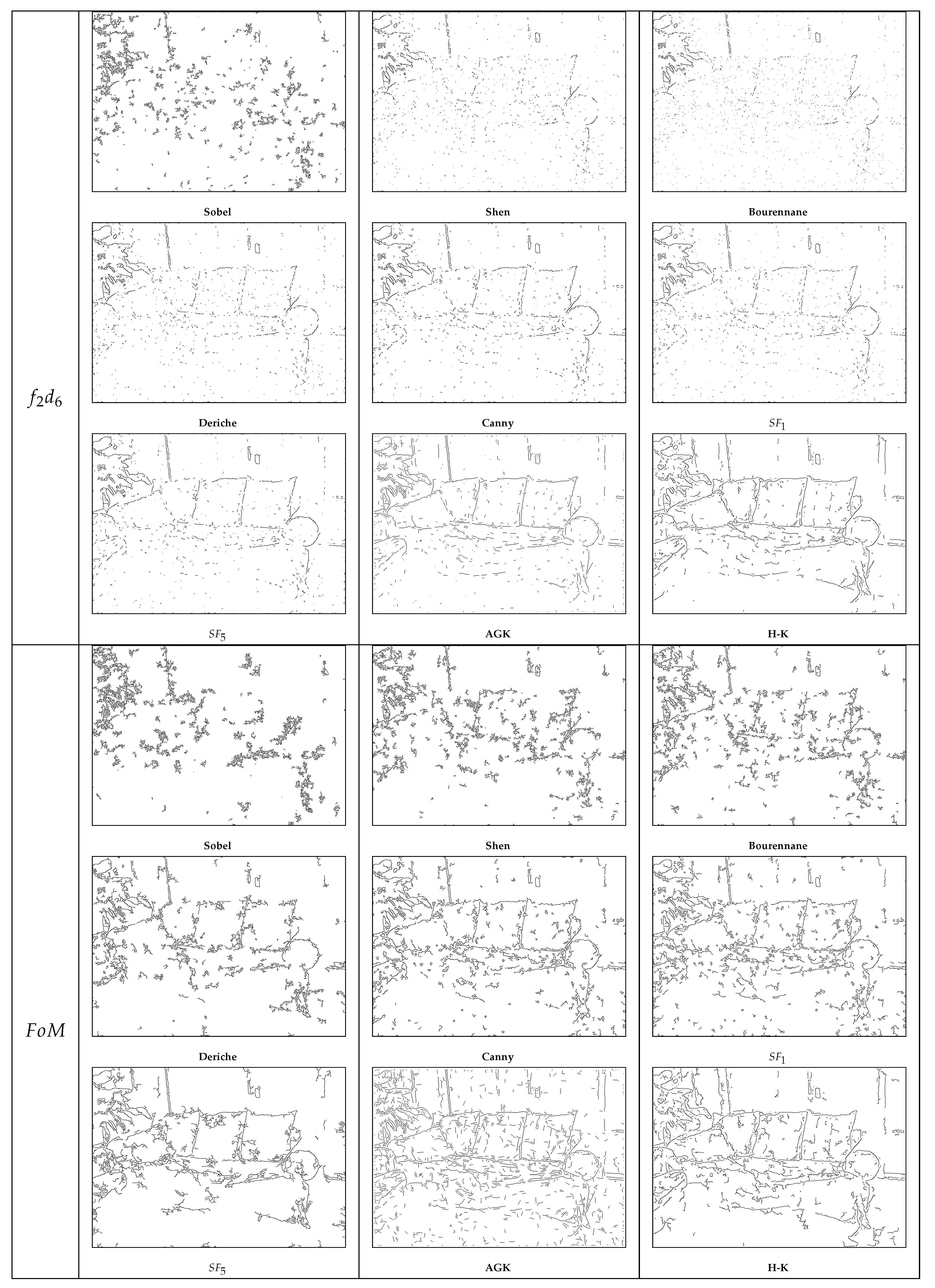
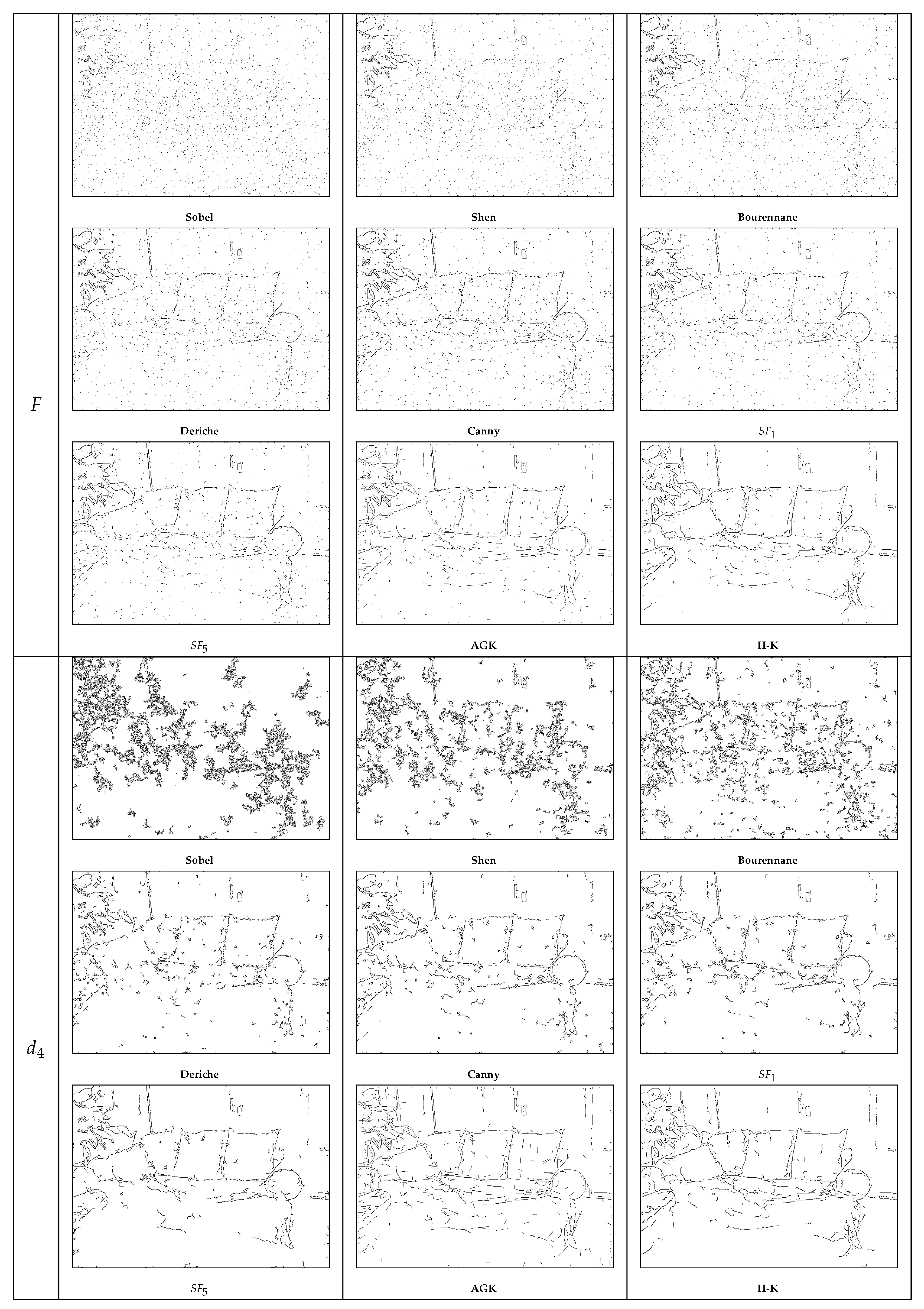
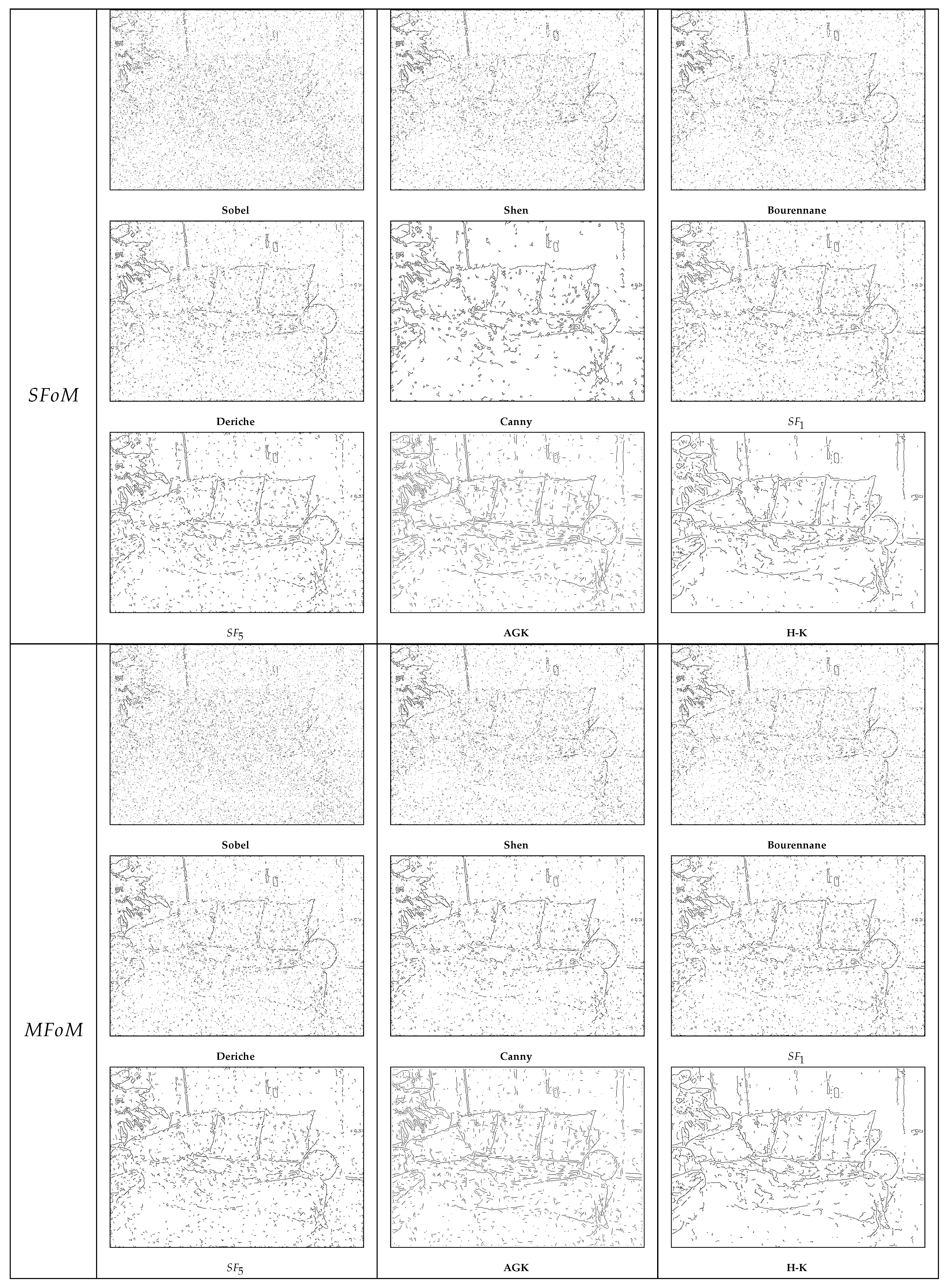
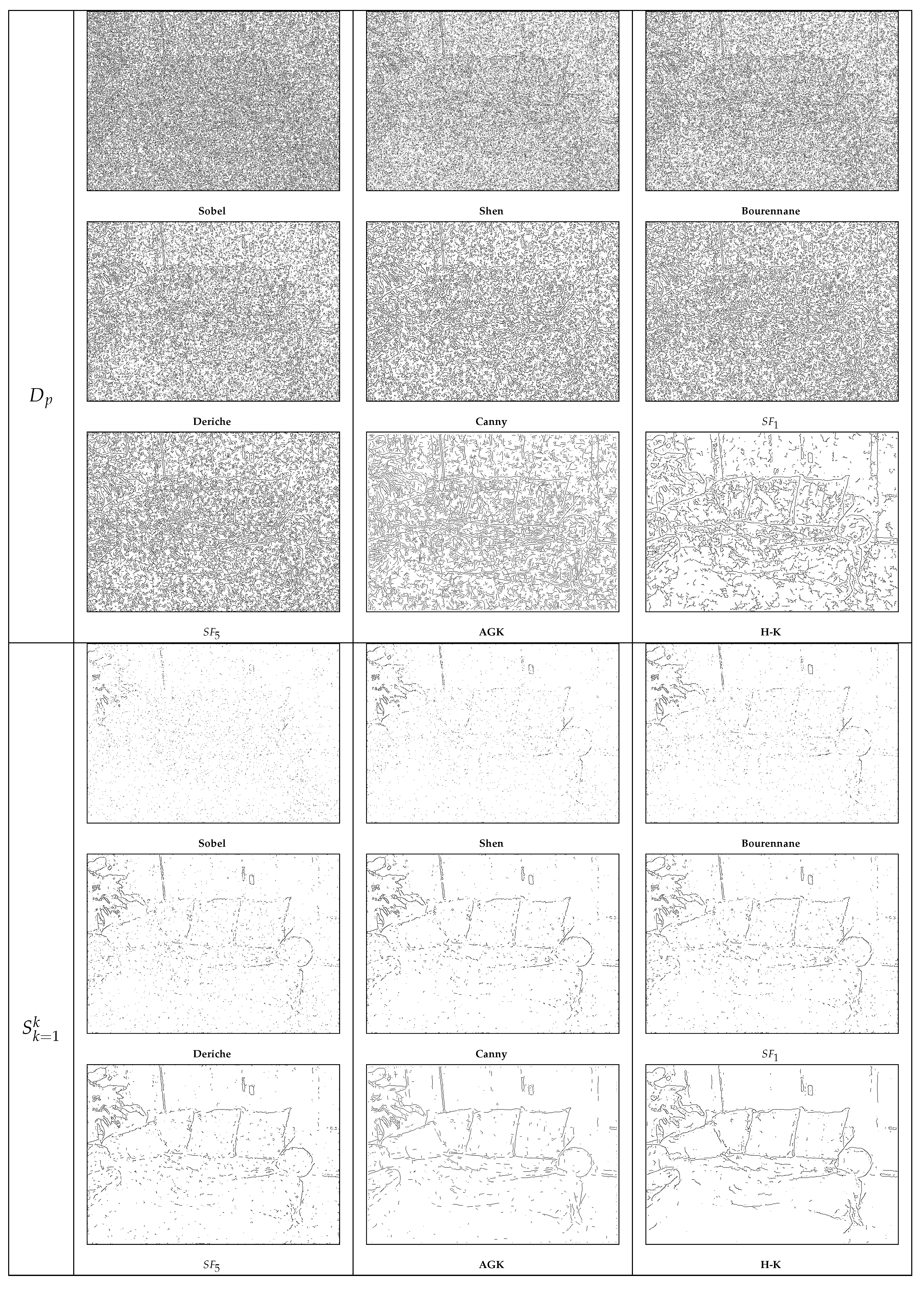
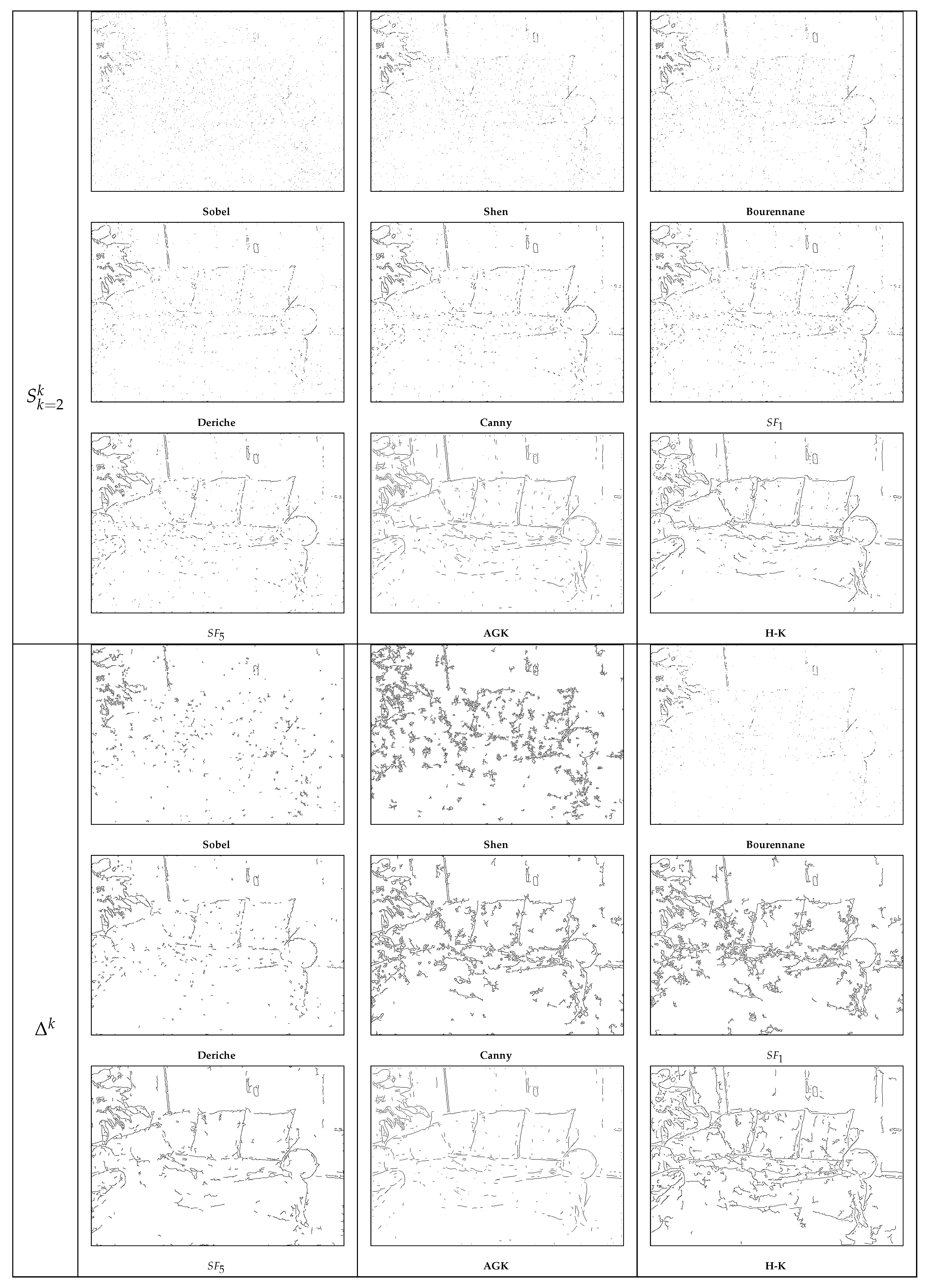
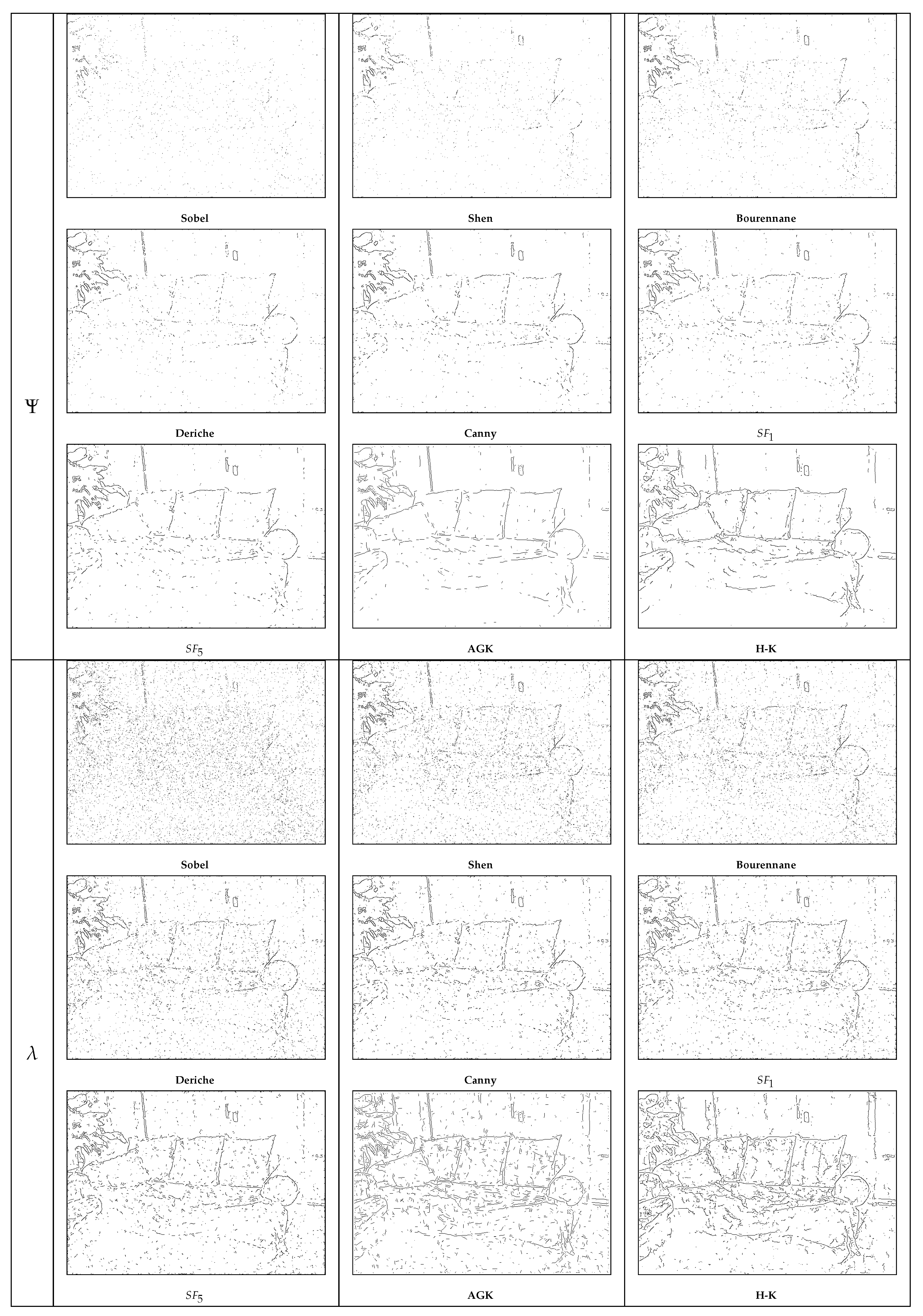
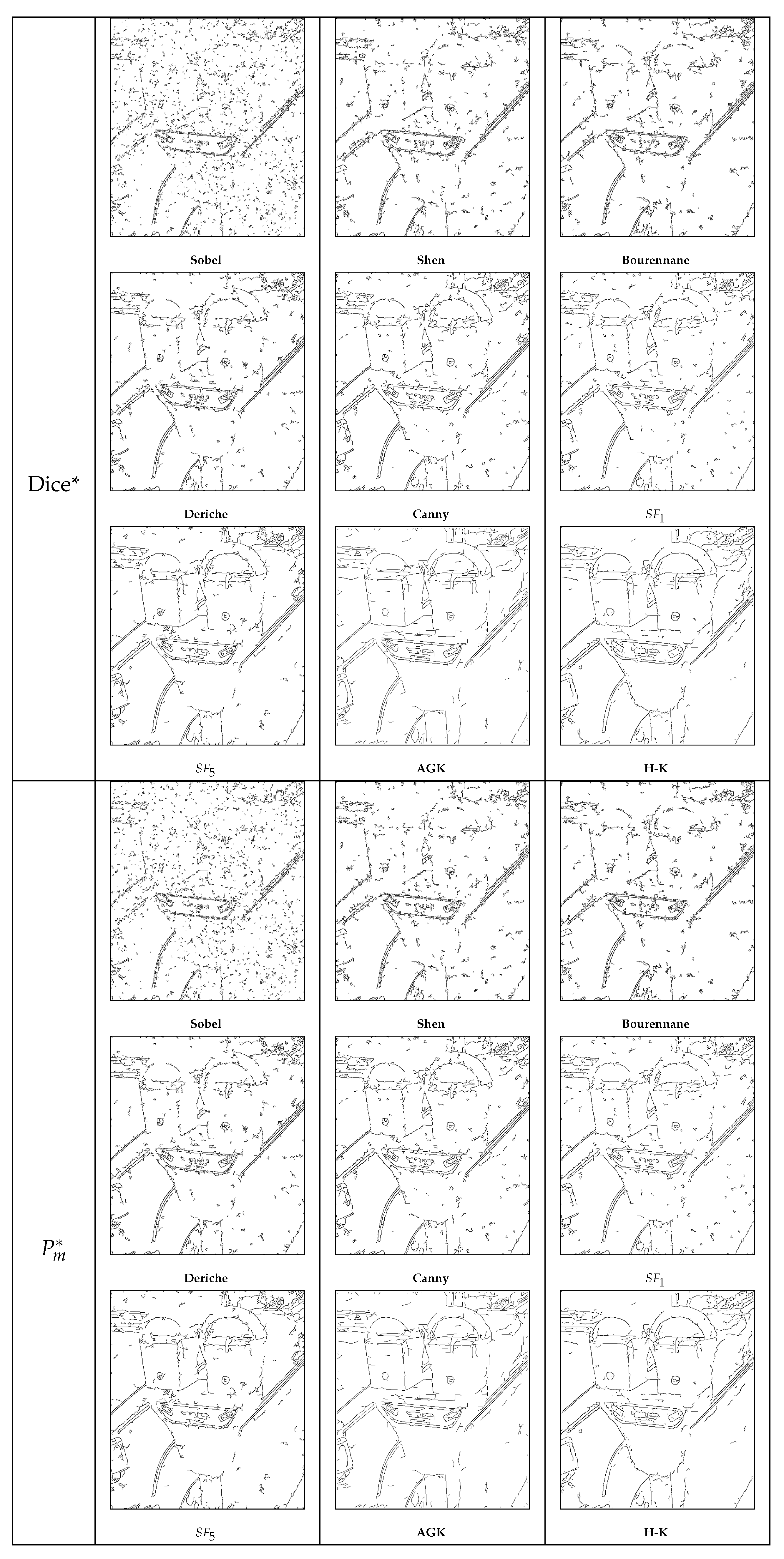
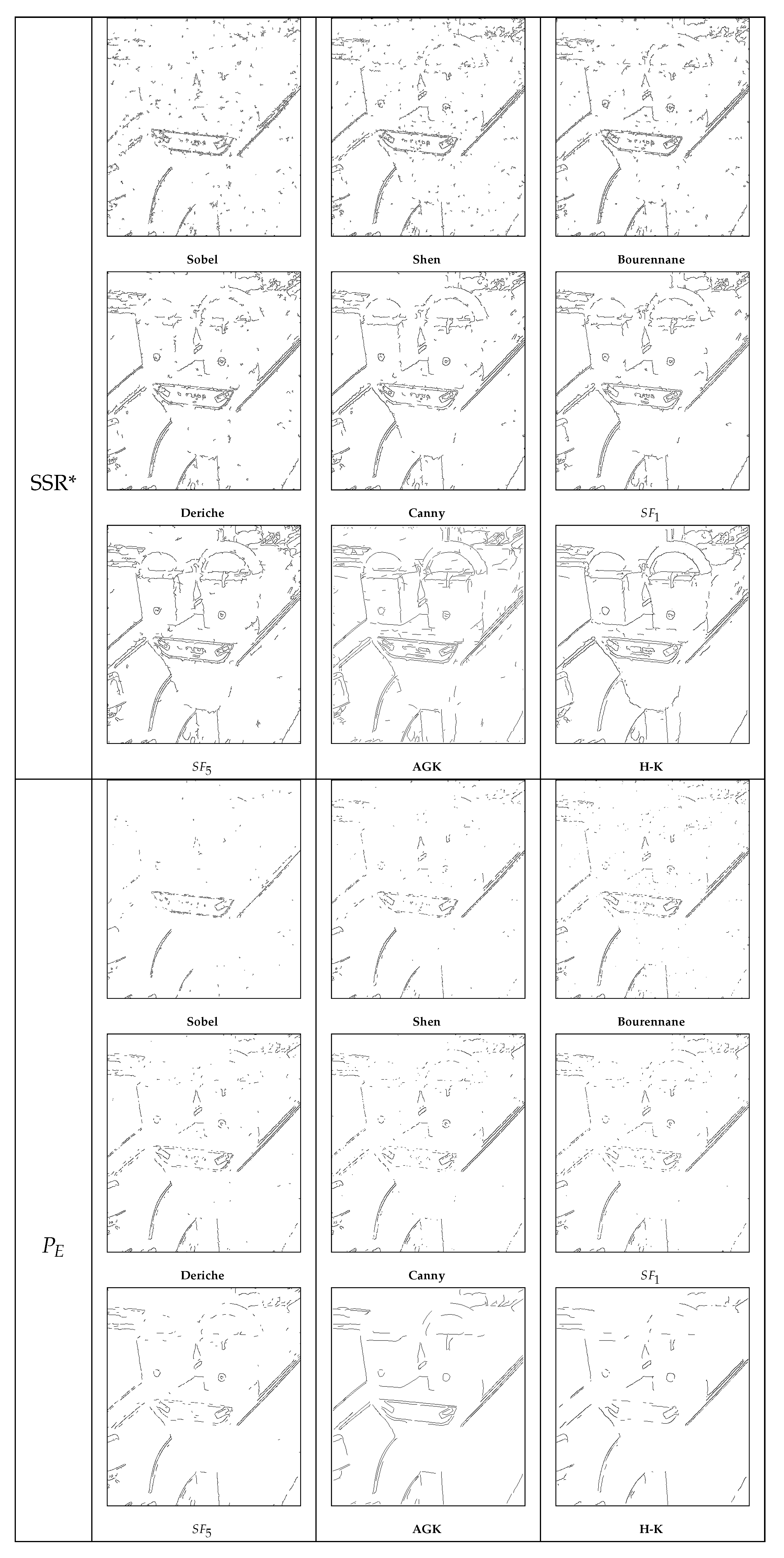
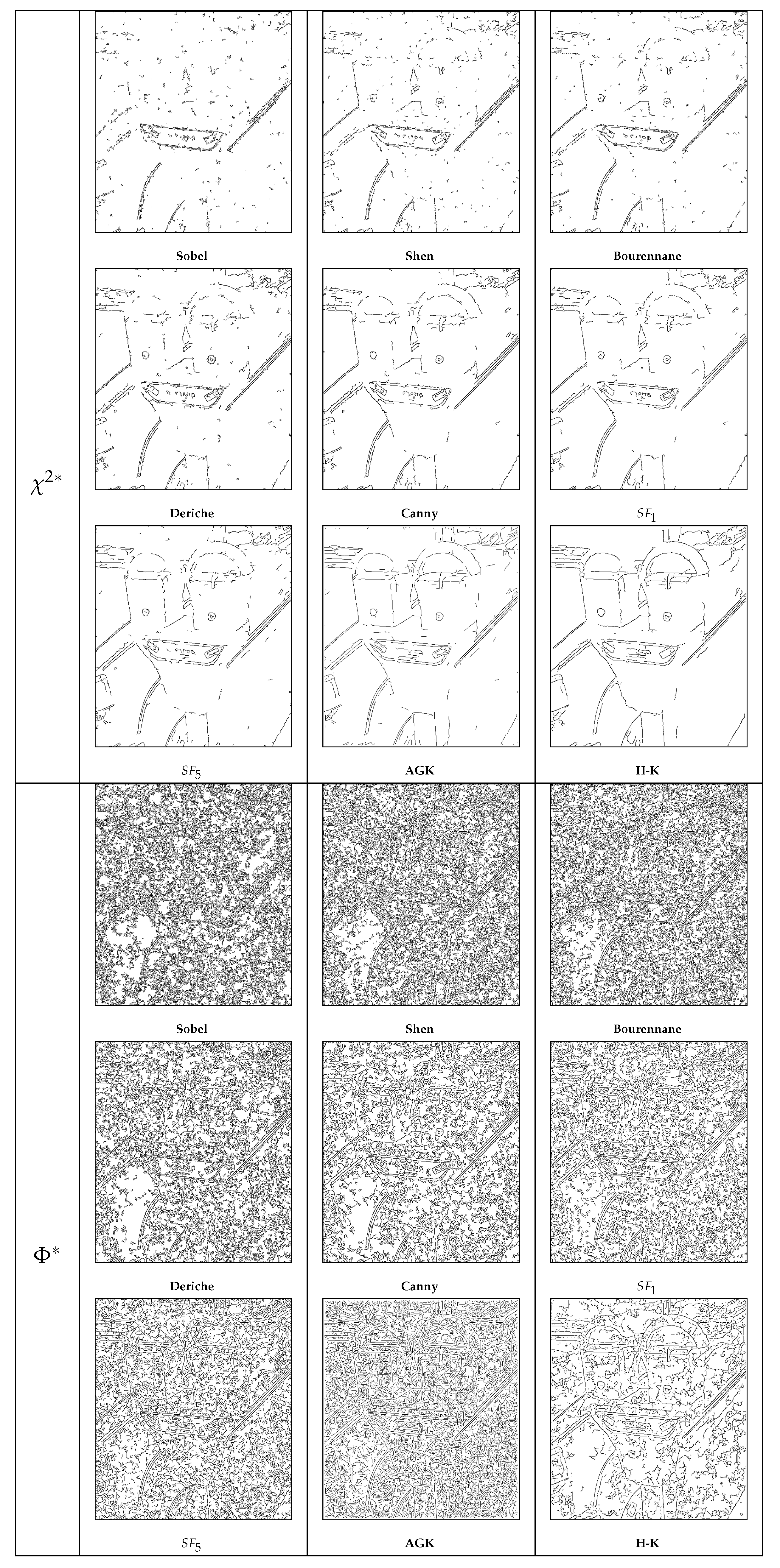
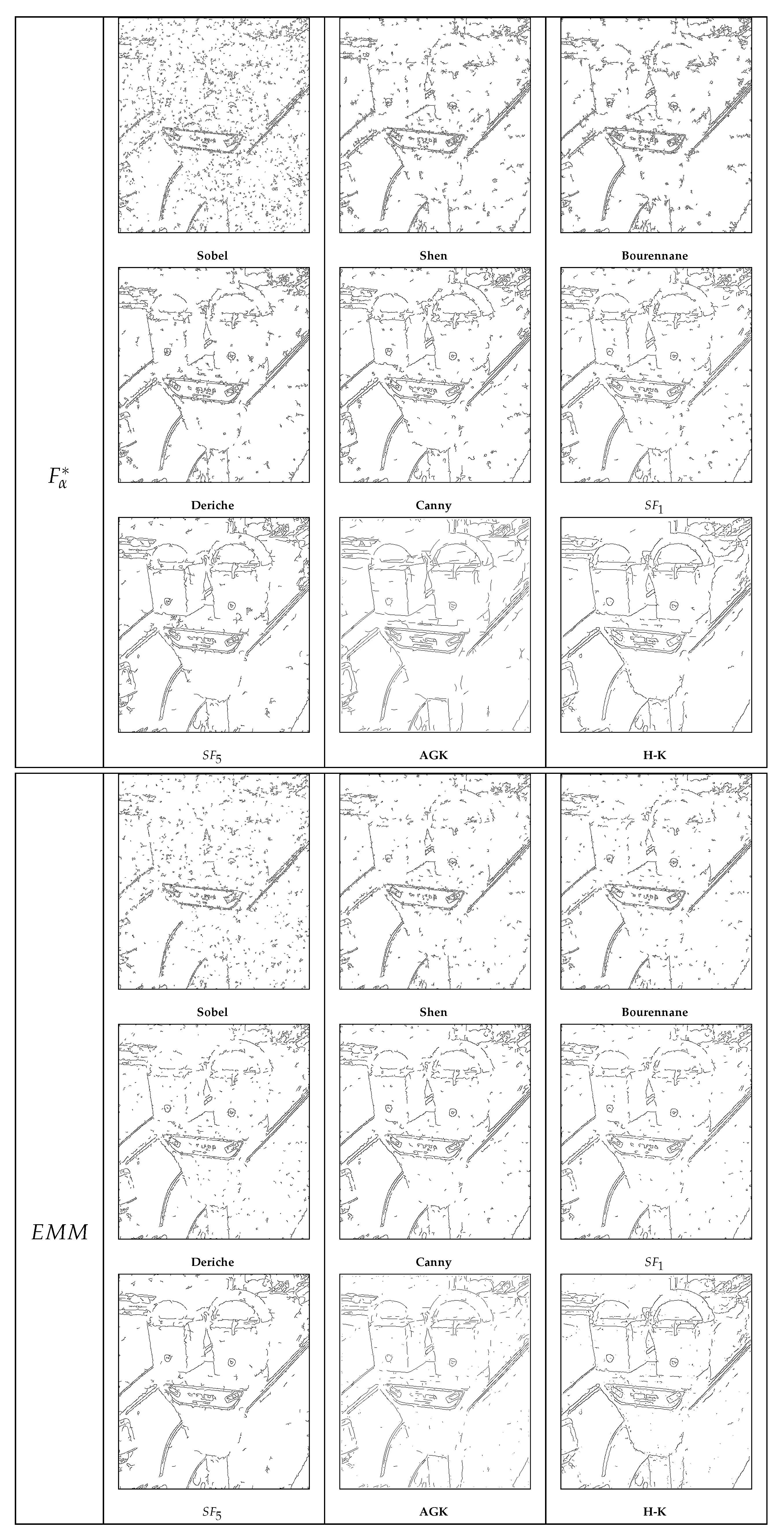
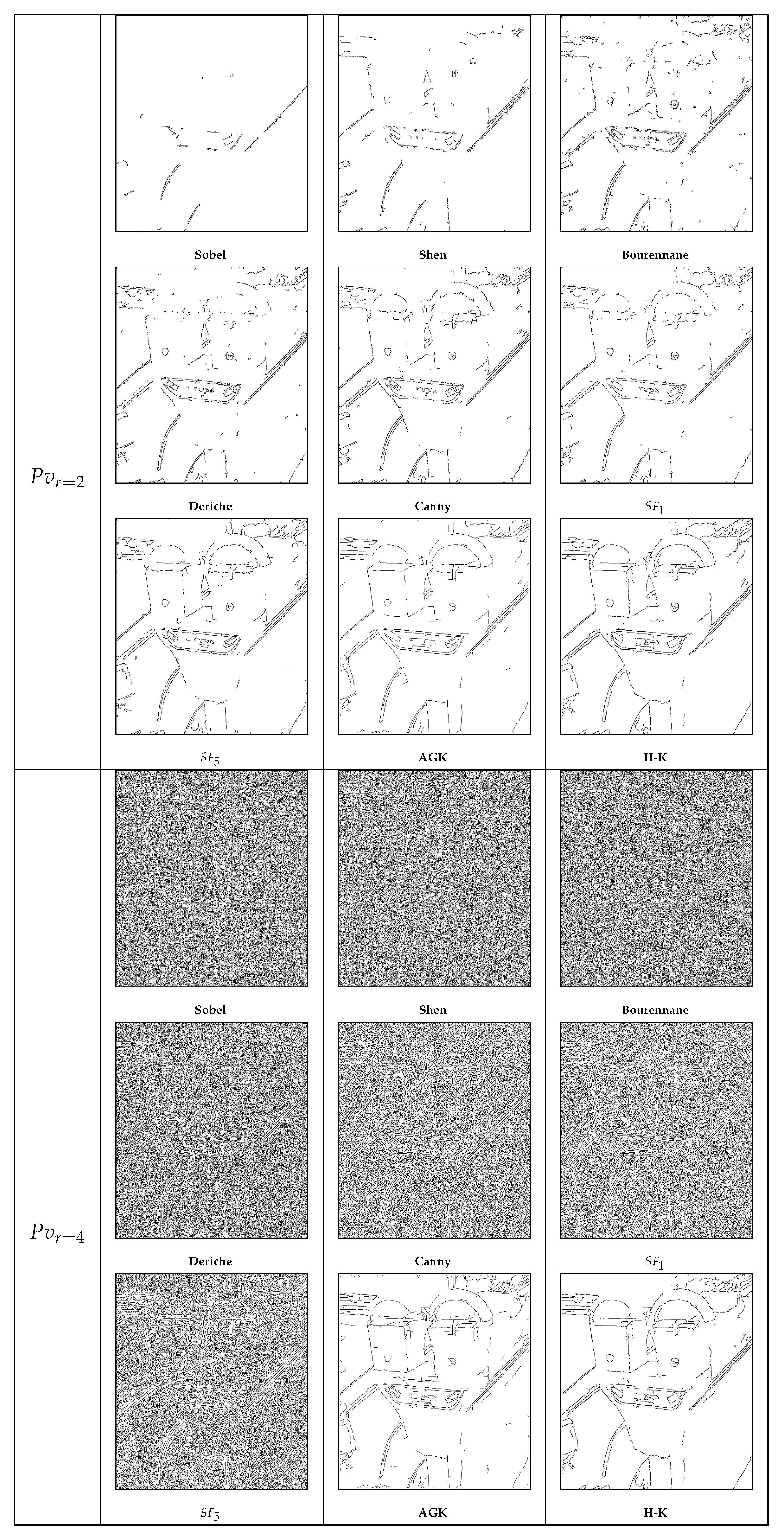
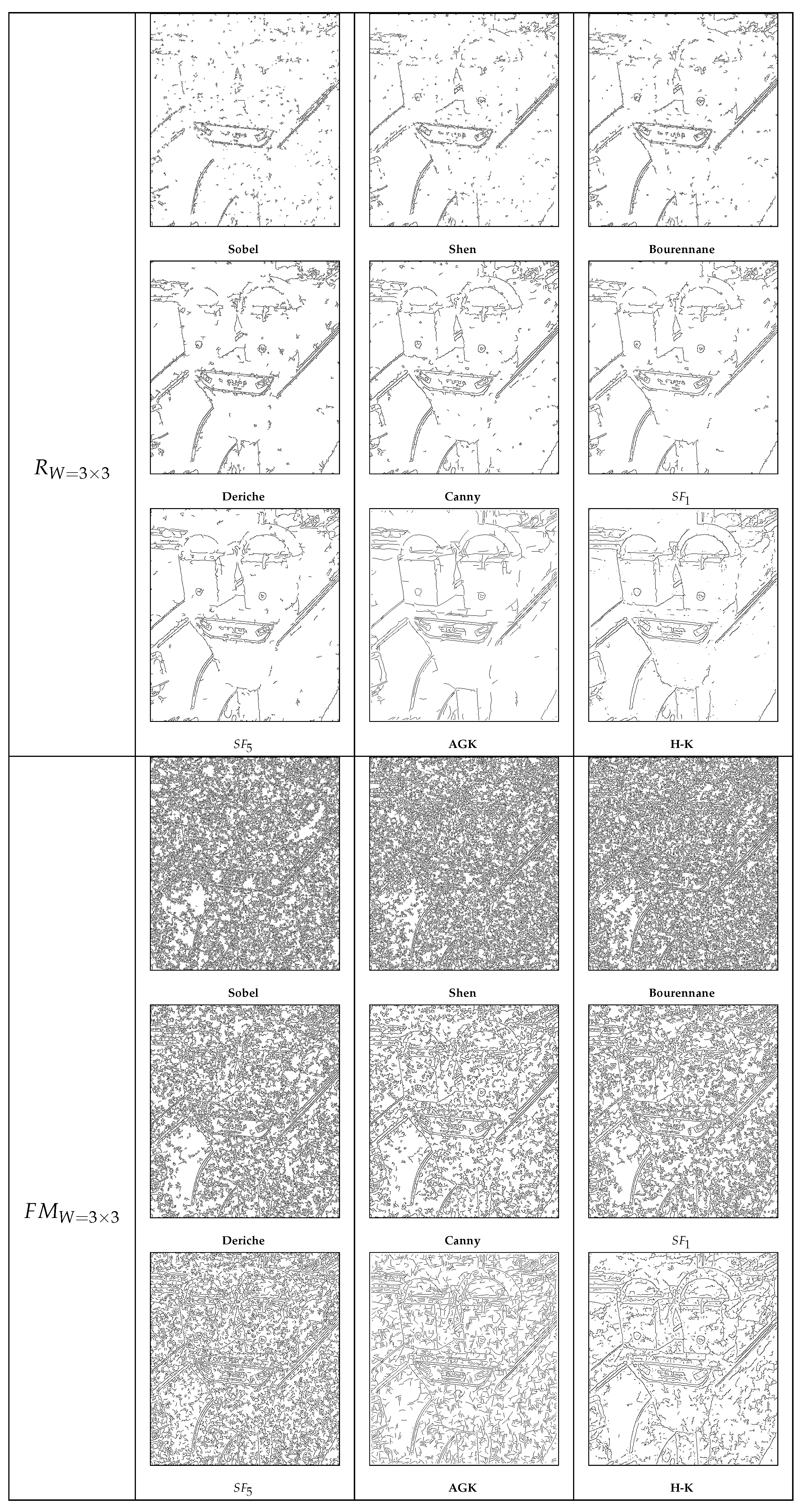
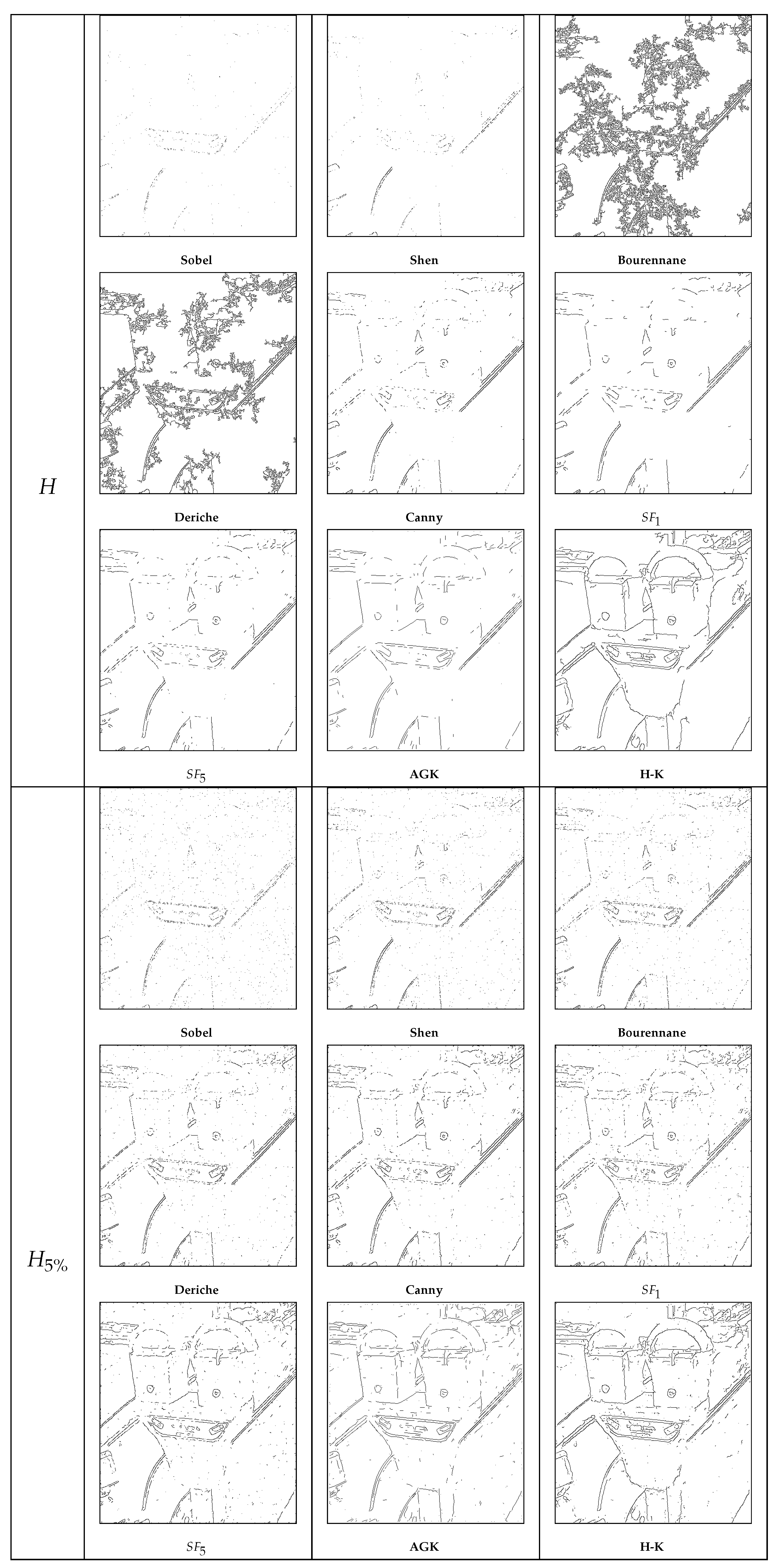
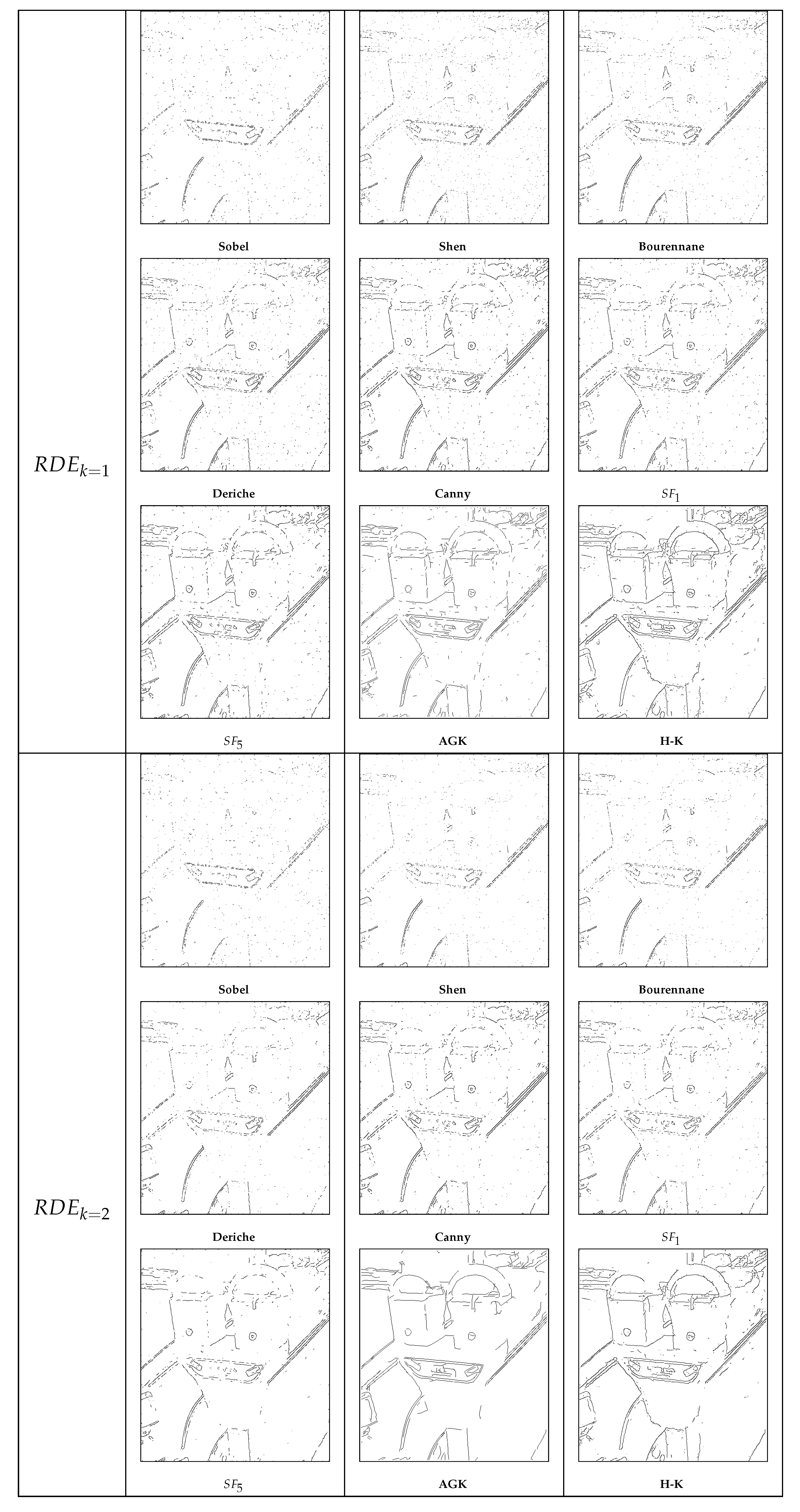
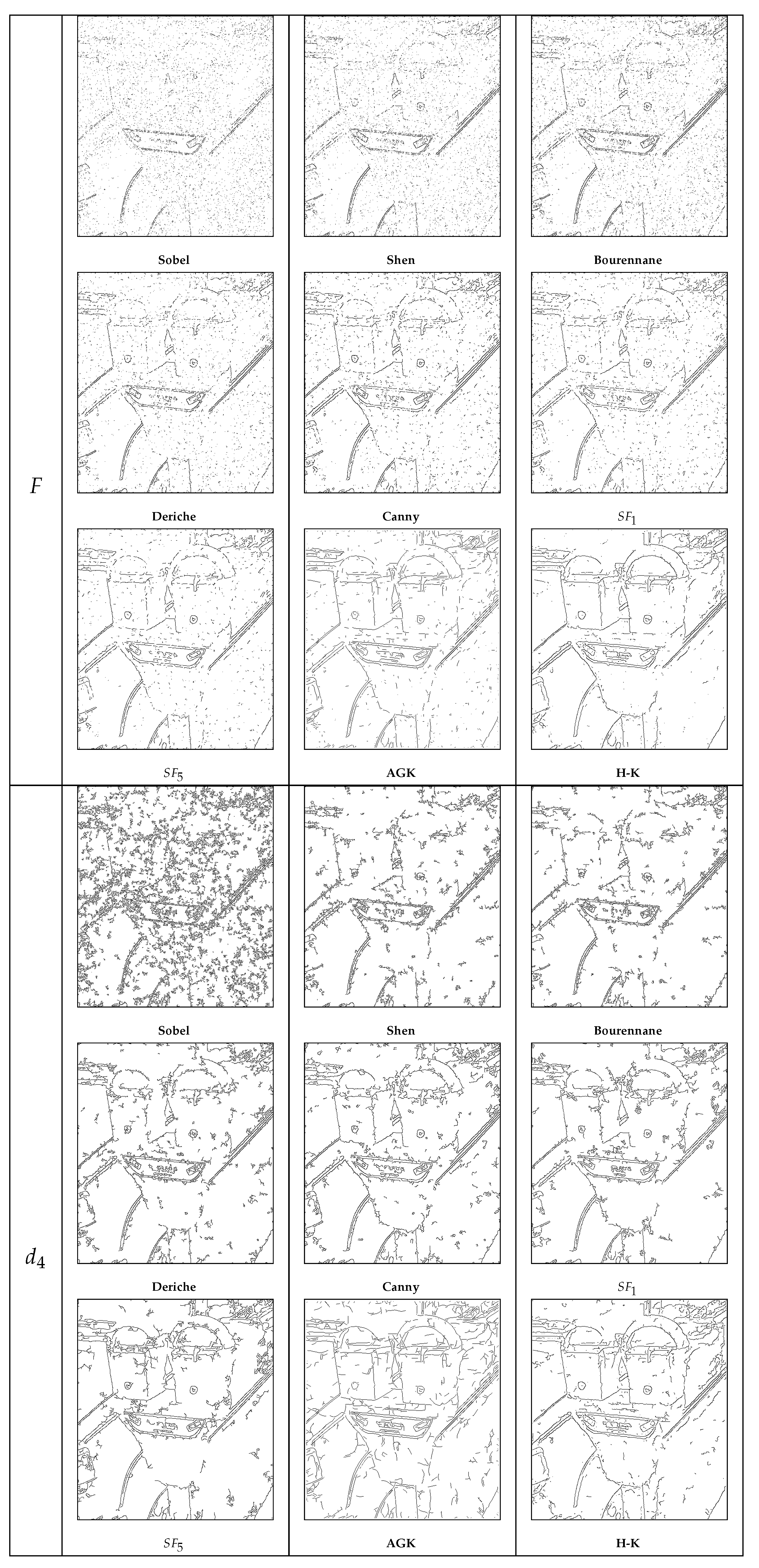
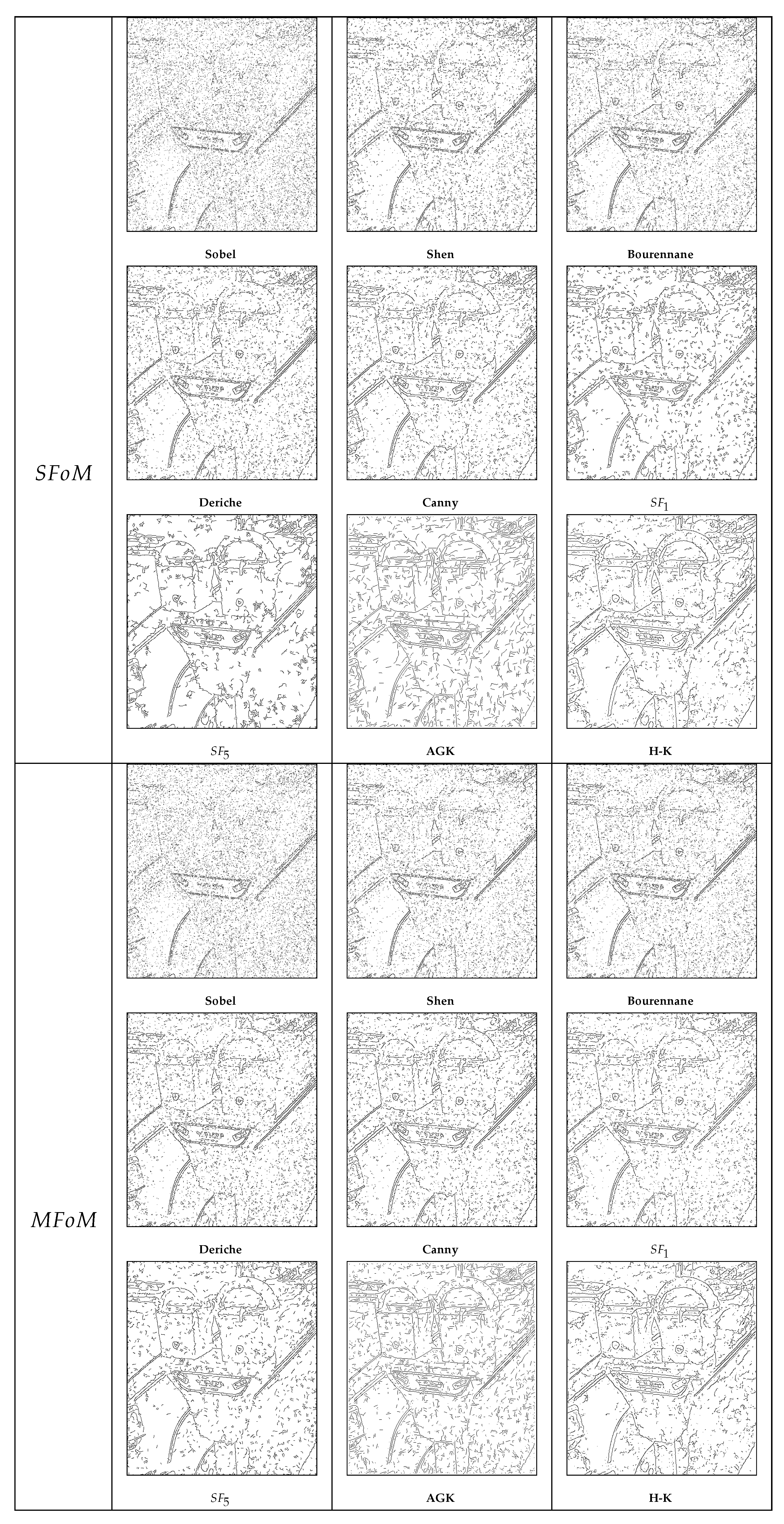
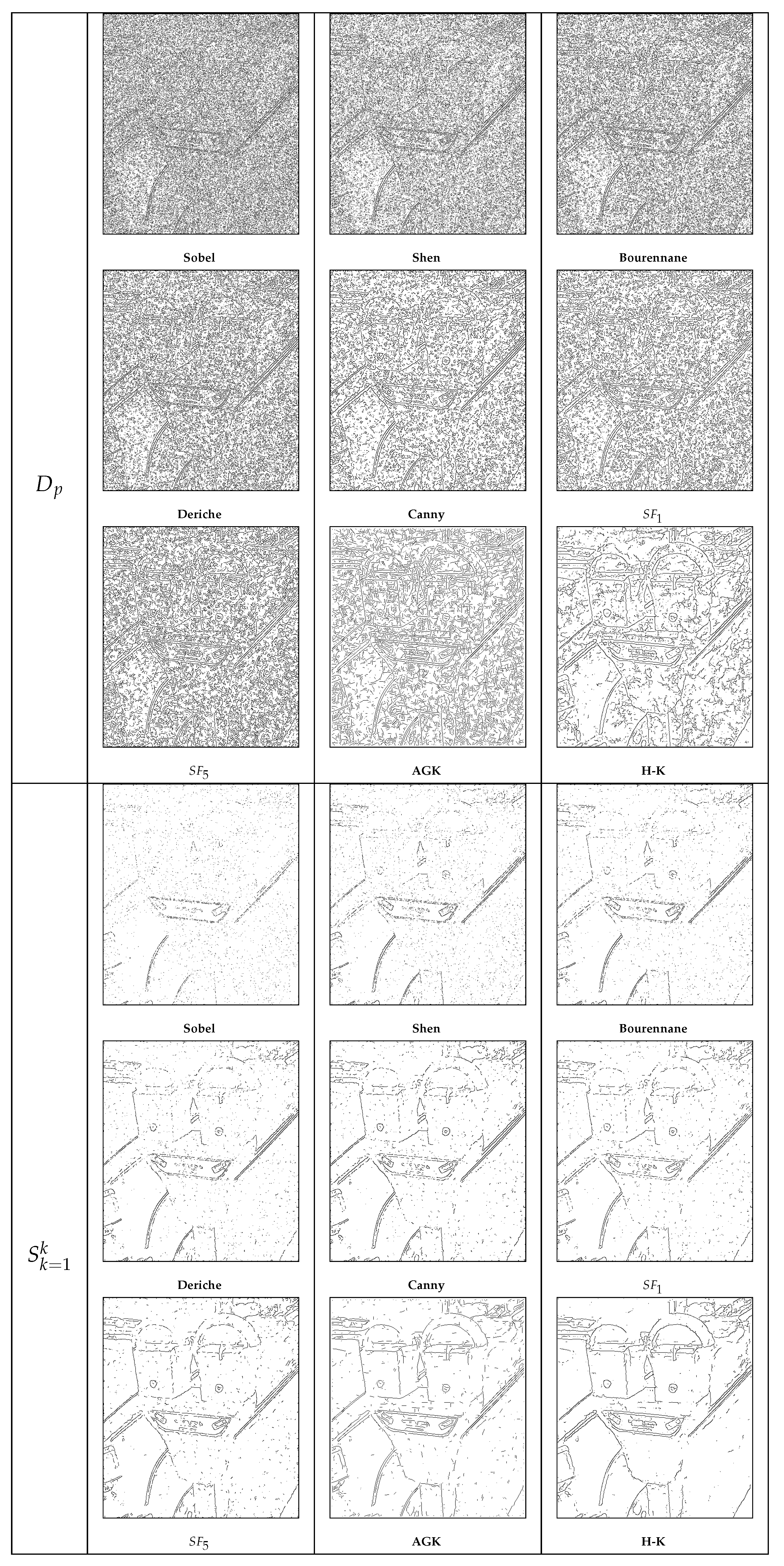
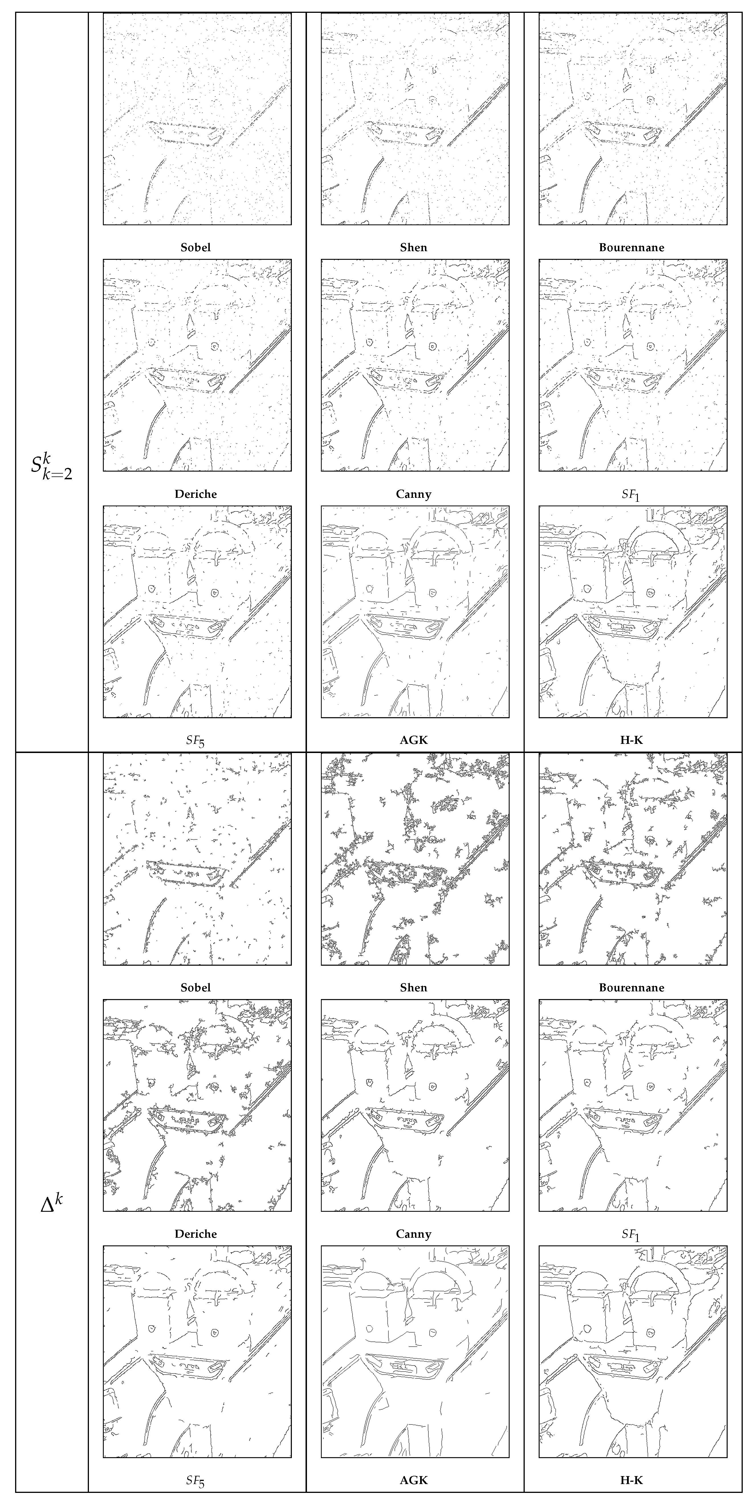
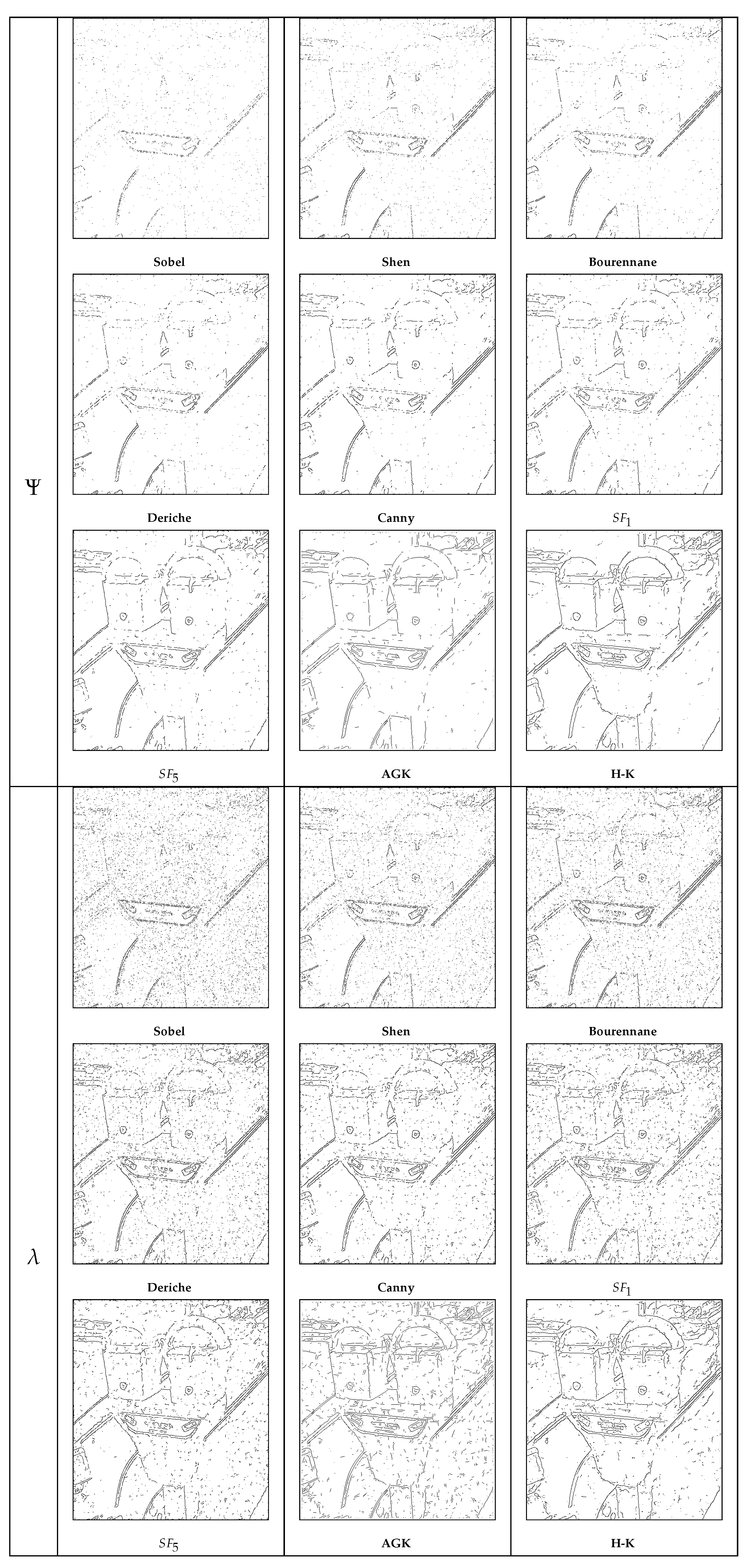
Firstly, the segmented images tied to corrupted images with PSNR = 14 dB, representing the best edge quality map for 28 different measures, are presented in Figure 20, Figure 21, Figure 22, Figure 23, Figure 24, Figure 25, Figure 26, Figure 27, Figure 28, Figure 29, Figure 30, Figure 31, Figure 32, Figure 33, Figure 34, Figure 35, Figure 36, Figure 37, Figure 38, Figure 39, Figure 40, Figure 41, Figure 42, Figure 43, Figure 44, Figure 45, Figure 46 and Figure 47. The results concerning over- and under-segmentation measures (cf. Section 2.3) are not reported because the score will always attain 0 for the best edge map which are either full of FPs or devoid of any contour point [14]. The edge map obtained using the Sobel filter is complicated; indeed, this filter is very sensitive to the noise in the image, so only few edge points will be correctly detected, the rest being FPs. Furthermore, thin edges (before thresholding) obtained using Shen, Bourennane and Deriche filters are not reliable, and it is difficult to choose/compute correct thresholds in order to visualize continuous objects’ contours. Segmentations obtained by $Dic{e}^{\ast }$, $P_m^{\ast }$ and $F_{\alpha }^{\ast }$ are overall visible, with a little too many FPs, except for AGK and H-K, which are correctly segmented. On the contrary, contour points concerning $SS{R}^{\ast }$ and ${\chi }^2\ast$ are less corrupted by FPs, but true edges are missing; in addition, edge maps concerning $P_E$ are worse. Edge maps tied to ${\mathsf{\Phi }}^{\ast }$, $F{M}_W$ and $D_p$ are hugely corrupted by FPs, since most of the object contours remain unidentifiable. Concerning $P_v$, either edges are missing, when $r=2$, or too many FPs appear, when $r=4$. Edge maps obtained by $R_W$ evaluation measures are adequate, even though object contours are not really visible concerning Shen, Bourennane and Deriche filters and some spurious pixels appear concerning AGK and H-K (cf. parkingmeter image). The Hausdorff distance H and ${\Delta }^k$ measures are not reliable because edge maps tied to these evaluations are either too noisy, or most edges are missing (except for H-K). The edge maps associated with $H_{5\%}$, $f_2{d}_6$, $S_{k=2}^k$ and $\psi$ are similar: not too many FPs, but edges with Shen, Bourennane and Deriche filters are not continuous. However, edges obtained using $f_2{d}_6$ are too noisy with AGK and H-K (cf. “parkingmeter” image), and the same remark applies to $S_{k=1}^k$ for AGK. Concerning $S^k$, note that, when $k=1$, edges are more easily visible than using $k=2$ because the distance measure score expands rapidly for a missing point far from its true position (demonstrated in [21]). For image 109, edges obtained by $EMM$ are not really continuous with the Shen, Bourennane, Deriche and Canny filters, whereas spurious pixels appears for the edges of the “parkingmeter” image. The edge maps obtained using minimum score of $FoM$ are heavily corrupted by continuous FPs, like hanging objects. This phenomenon is always present, but less pronounced, with $d_4$. Edge maps are too corrupted by FPs with $MFoM$ and $SFoM$, even though objects are visible, whereas FPs remains less present using F and $\lambda$. The segmentations tied to $RDE$ are reliable, not too many FPs, although some edges are missing. Lastly, the edges maps using the proposed measure $\mathsf{\Xi }$ are not corrupted by noise, the objects are visible, even with the Shen, Bourennane and Deriche filters. In addition, edge maps for Canny and $S{F}_1$ are particularly well segmented.

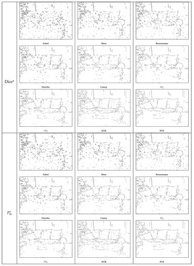
Figure 20. Ideal segmentations for several edge detectors on image 109, PSNR = 14 dB.

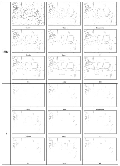
Figure 21. Ideal segmentations for several edge detectors on image 109, PSNR = 14 dB.

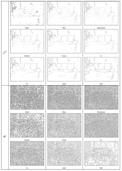
Figure 22. Ideal segmentations for several edge detectors on image 109, PSNR = 14 dB.

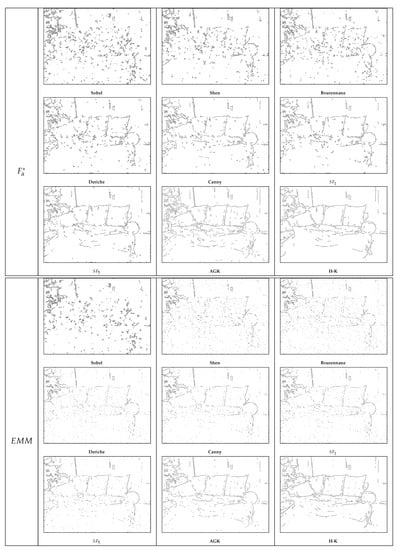
Figure 23. Ideal segmentations for several edge detectors on image 109, PSNR = 14 dB.

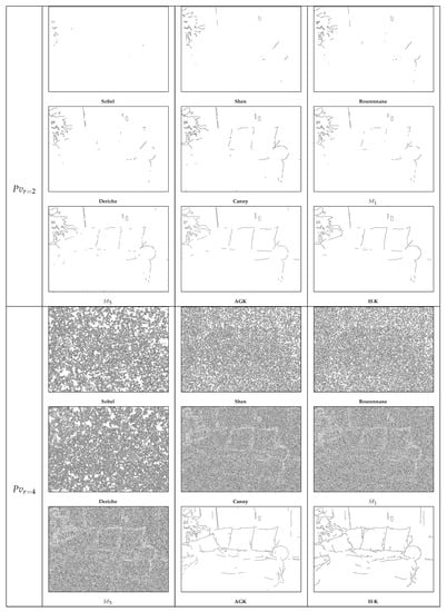
Figure 24. Ideal segmentations for several edge detectors on image 109, PSNR = 14 dB.

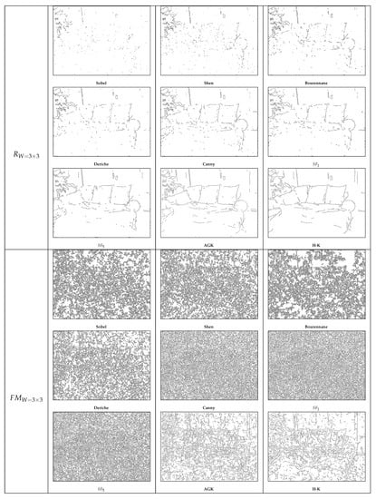
Figure 25. Ideal segmentations for several edge detectors on image 109, PSNR = 14 dB.

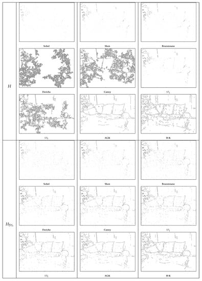
Figure 26. Ideal segmentations for several edge detectors on image 109, PSNR = 14 dB.

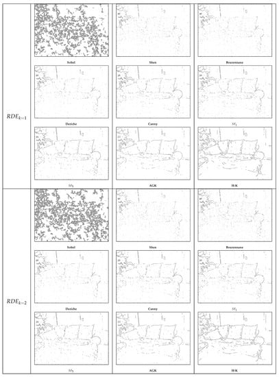
Figure 27. Ideal segmentations for several edge detectors on image 109, PSNR = 14 dB.

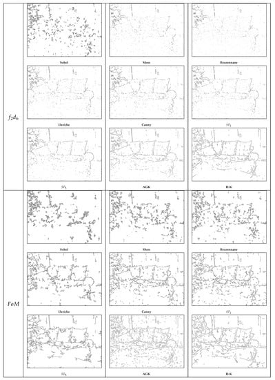
Figure 28. Ideal segmentations for several edge detectors on image 109, PSNR = 14 dB.

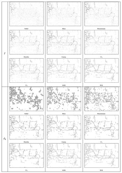
Figure 29. Ideal segmentations for several edge detectors on image 109, PSNR = 14 dB.

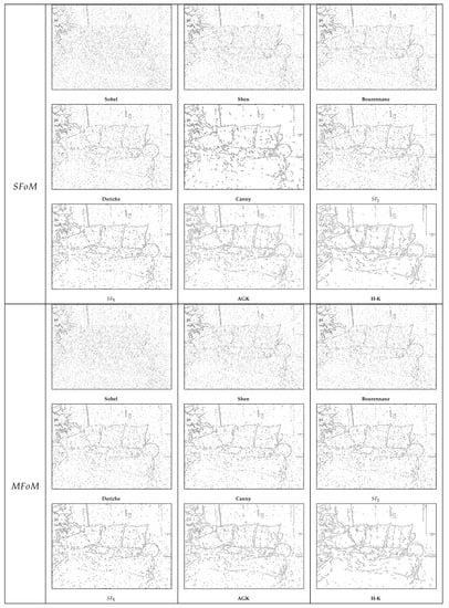
Figure 30. Ideal segmentations for several edge detectors on image 109, PSNR = 14 dB.

Figure 31. Ideal segmentations for several edge detectors on image 109, PSNR = 14 dB.

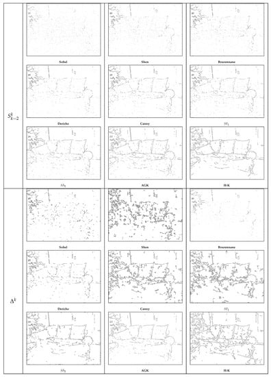
Figure 32. Ideal segmentations for several edge detectors on image 109, PSNR = 14 dB.

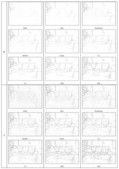
Figure 33. Ideal segmentations for several edge detectors on image 109, PSNR = 14 dB.

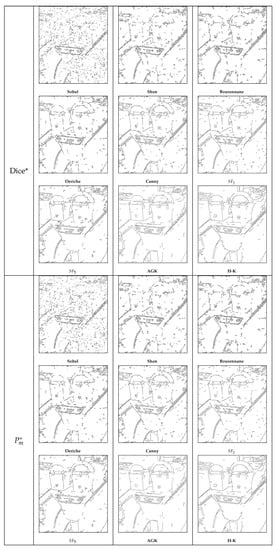
Figure 34. Ideal segmentations for several edge detectors on image parkingmeter, PSNR = 14 dB.

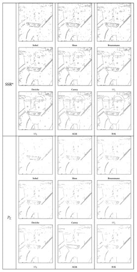
Figure 35. Ideal segmentations for several edge detectors on image parkingmeter, PSNR = 14 dB.

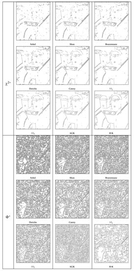
Figure 36. Ideal segmentations for several edge detectors on image parkingmeter, PSNR = 14 dB.

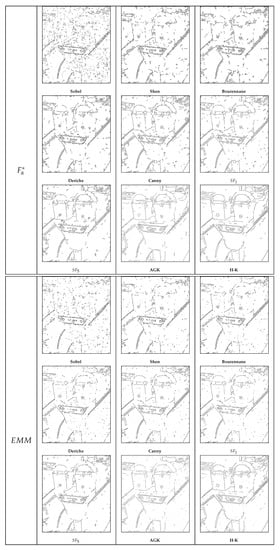
Figure 37. Ideal segmentations for several edge detectors on image parkingmeter, PSNR = 14 dB.

Figure 38. Ideal segmentations for several edge detectors on image parkingmeter, PSNR = 14 dB.

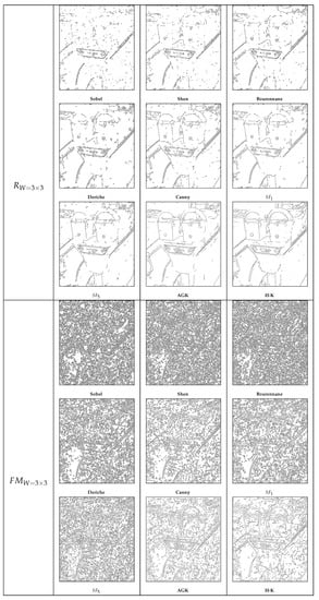
Figure 39. Ideal segmentations for several edge detectors on image parkingmeter, PSNR = 14 dB.

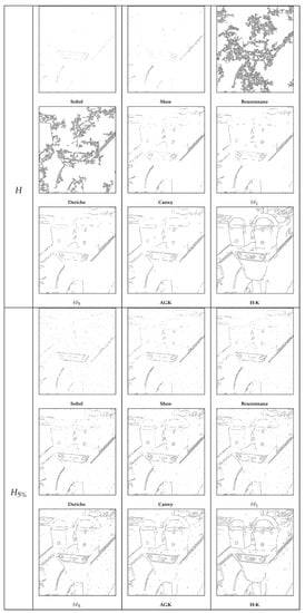
Figure 40. Ideal segmentations for several edge detectors on image parkingmeter, PSNR = 14 dB.

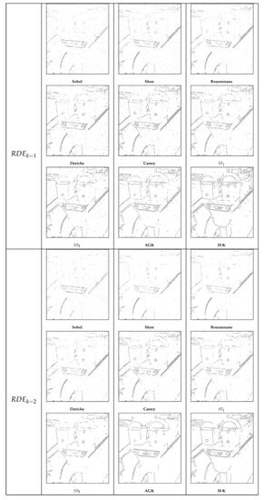
Figure 41. Ideal segmentations for several edge detectors on image parkingmeter, PSNR = 14 dB.

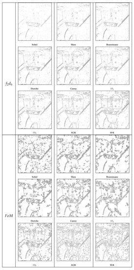
Figure 42. Ideal segmentations for several edge detectors on image parkingmeter, PSNR = 14 dB.

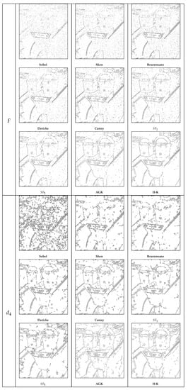
Figure 43. Ideal segmentations for several edge detectors on image parkingmeter, PSNR = 14 dB.

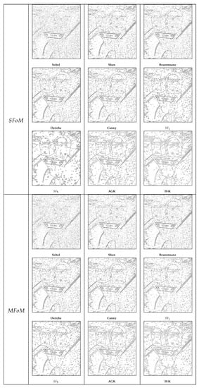
Figure 44. Ideal segmentations for several edge detectors on image parkingmeter, PSNR = 14 dB.

Figure 45. Ideal segmentations for several edge detectors on image parkingmeter, PSNR = 14 dB.

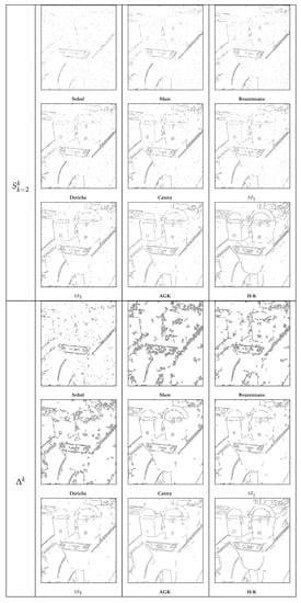
Figure 46. Ideal segmentations for several edge detectors on image parkingmeter, PSNR = 14 dB.

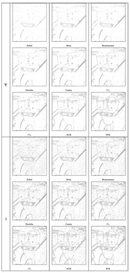
Figure 47. Ideal segmentations for several edge detectors on image parkingmeter, PSNR = 14 dB.

Secondly, the plotted curves available in Figure 18 and Figure 19 evolve as a function of the noise level (Gaussian noise). The noise level is represented by PSNR values: from 17 dB to 10 dB. Consequently, the measure scores and the noise level must increase simultaneously. Moreover, scores of the evaluation measures associated with the Sobel filter, which is sensitive to noise, must be higher than other measures; scores concerning Shen and Bourennane filters must be situated just bellow. Finally, measure scores tied to $S{F}_5$, AGK and H-K must be plotted at the bottom, and, scores associated with Canny, Deriche and $S{F}_1$ filters must be situated above, but below the Shen and Bourennane filters. Now, scores of $Dic{e}^{\ast }$, $P_m^{\ast }$, $SS{R}^{\ast }$, ${\chi }^2\ast$ and $F_{\alpha }^{\ast }$ measures increase monotonously, but these scores are not consistent with the computed edge maps. Indeed, considering the segmented images presented with PSNR = 14 dB, scores concerning Canny and $S{F}_1$ filters are better than H-K, whereas the H-K segmentation is of higher quality than others (continuous contours, less spurious pixels). Concerning $P_E$, in particular, this measure qualifies the Sobel, Shen and Bourennane filters better than H-K. Similarly, ${\mathsf{\Phi }}^{\ast }$, $F{M}_W$, $D_p$ and $\mathsf{\Psi }$ qualify H-K and AGK as the worse edge detectors. Concerning $P_v$, either curves are confused, when $r=2$, or scores are negative, when $r=4$. By contrast, H, $H_{5\%}$ and ${\Delta }^k$ scores have a random behavior, even though $H_{5\%}$ seems better, but not reliable (see H-K or Sobel scores as examples). The curves for $FoM$, F, $d_4$ and $MFoM$ are mixed and confused, F qualifies Shen and Bourennane filters as the best edge detectors, whereas H-K and AGK are qualified as the worst. The Deriche filter appears as the best edge detector for $d_4$, although the segmentation using H-K is clearly better. Curves are mixed using $SFoM$ for the “parkingmeter” image. These plotted scores are consistent with the images of segmentation, which are heavily corrupted by FPs. No filter can be really qualified as better than the others. It is also a similar case for $\lambda$, where the scores are confused, except with the Sobel filter. Concerning $S_{k=2}^k$, the plotted scores remain unreliable, cf. AGK scores. When $k=1$, $S^k$ scores evolve properly, even though $S{F}_5$ is penalized as strongly as the Canny filter. Therefore, the measures having the correct evolution with the correct filter qualification are $EMM$, $R_W$, $RDE$, $f_2{d}_6$ and $S_{k=1}^k$. The scores obtained by $\mathsf{\Xi }$ are presented in Figure 48 and Figure 49, where FP and FN distances are also reported. Although these distances do not evolve monotonously, the final score remains monotonous and the qualifications of the filters are reliable. Actually, the weights concerning FN distances allow a reliable final computation of $\mathsf{\Xi }$ scores. Finally, the results gathering reliability of the segmentation, curve evolution and filter qualification for each edge detection evaluation are summarized in Table 5.

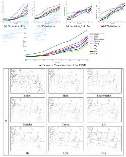
Figure 48. Segmentations and scores concerning $\mathsf{\Xi }$ measure and image 109.

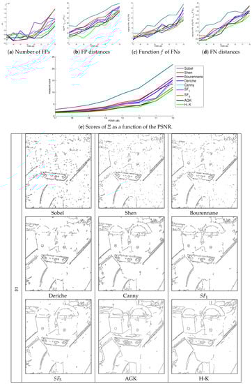
Figure 49. Segmentations and scores concerning $\mathsf{\Xi }$ measure and image parkingmeter.

Table 5. Reliability of the reviewed edge detection evaluation measures.

Measure	Segmentation Reliability	Monotonic Curves	Filter Qualification
$Dic{e}^{\ast }$	≈	✓	✗
$P_m^{\ast }$	≈	✓	✗
$SS{R}^{\ast }$	≈	✓	✗
$P_E$	✗	✓	✗
${\chi }^{2\ast }$	≈	✓	✗
${\mathsf{\Phi }}^{\ast }$	✗	✓	✗
$F_{\alpha }^{\ast }$	≈	✓	✗
$P{v}_{r=2}$	✗	✓	≈
$P{v}_{r=4}$	✗	✓	✗
$R_W$	✓	✓	≈
$F{M}_W$	✗	✓	✗
H	✗	✗	✗
${\Delta }^k$	✗	✗	✗
$H_{5\%}$	≈	✗	✗
$FoM$	✗	✓	✗
F	≈	✓	✗
$d_4$	≈	✓	✗
$SFoM$	≈	✓	✗
$MFoM$	≈	✓	✗
$D_p$	✗	✓	✗
$EMM$	≈	✓	✓
$f_2{d}_6$	≈	✓	✓
$RD{E}_{k=1}$	✓	✓	✓
$RD{E}_{k=2}$	✓	≈	✓
$S_{k=1}^k$	≈	✓	≈
$S_{k=2}^k$	≈	✓	✗
$\mathsf{\Psi }$	≈	✓	✗
$\lambda$	≈	✓	≈
$\mathsf{\Xi }$	✓	✓	✓

5. Conclusions

This study presents a survey of supervised edge detection evaluation methods. Several techniques are based on the number of false positive, false negative, true positive and/or true negative points. Other methods strongly penalize misplaced points when they are outside a window centered on a true point. In addition, many approaches compute the distance from the position where a contour point should be located. Most of these edge detection assessment methods are presented here, with many examples, exposing the drawbacks for different comparisons of edges with different shapes. Measures involving only statistics fail to assess objectively when there are no common edge points between the ground truth ($G_t$) and the desired contour ($D_c$). On the contrary, assessments involving spatial areas around edges (i.e., windows around a point) remain unreliable if several points are detected for one contour point. Moreover, these techniques depend strongly on the window size, which enables misplaced points outside the considered window to be severely penalized. Among assessments involving spacial areas around edges, only the $R_W$ measure is suitable. Therefore, assessment involving distances of the misplaced pixels can evaluate a desired edge as a function of the distances between the ground truth edges and each point of $D_c$. There exist different implementations to assess edges using distances (Note that different strategies exist containing some operators other than confusion matrices of distances to assess edge detectors, they are referenced in [69].). On the one hand, some methods record only distances of false positive points, or only distances of false negative points. On the other hand, some assessment techniques are based on both distances of false positives (FPs) and false negative points (FNs). Among the more prominent measures, the Figure of Merit ($FoM$) remains the most widely used. The main drawback of this technique is that is does not consider distances of false negative points, i.e., false negative points are strongly penalized without considering their distances; consequently, two different desired contours can obtain the same evaluation, even if one of them if visually closer to the true edge. Consequently, several edge evaluation methods are derived from the Hausdorff distance, they compute both distances of FPs and FNs. The main differences between these edge detection evaluation measures are the weights for the FP and/or FN distances and the power tied to the distance computations. As FNs are often close to detected edges (TPs or FPs close to $G_t$), most error measures involving distances do not consider this particularity and are not sufficiently penalized. Distances of FPs strongly penalize edge detectors evaluated by the majority of these measures. Only $RD{E}_k$ computes the distances of FPs and FNs separately.

In order to objectively compare all these supervised edge detection assessment methods in an objective way, based on the theory of the dissimilarity evaluation measures, the objective evaluation assessed nine 1st-order edge detectors involving the minimum score of the considered measures by varying the parameters of the hysteresis. The segmentation that obtains the minimum score of a measure is considered as the best one. The scores of the different measures and different edge detectors are recorded and plotted as a function of the noise level in the original image. A plotted curve must increase monotonously with the noise level (Gaussian noise), represented by PSNR values (from 17 dB to 10 dB). It is proved that some edge detectors are better than others. The experiments show the importance of the growing increase of the noise level: a given edge evaluation measure can qualify an edge detector as low for a given noise level, whereas, for a higher noise level, the same edge detector obtains a better score. Consequently, mixing the results of curve evolution (monotonic or not), filter qualification (poor edge detector penalized stronger than robust edge detector) and the obtained edge map tied to the minimum score of a considered measure, a credible evaluation is obtained concerning the studied measures. These experiments exhibit the importance of dissociating both distances of FPs and FNs. A minimum of measures involving only statistics can be tied to correct segmented images, but the evolution of the scores is not reliable as a function of the edge detector robustness. On the contrary, edge maps are visually closer to the ground truth by considering the distance of false negative points tuned by a weighting. The same applies to the score evolution, and remains significant for edge detector qualification. The results gathering reliability of the segmentation, curve evolution and filter qualification for each edge detection evaluation are summarized in Table 5. Thus, the edge detection evaluations that are objectively suitable are the Relative Distance Error ($RD{E}_{k=1}$) and the new proposed measure $\mathsf{\Xi }$. The main difference between $RDE$ and $\mathsf{\Xi }$ is that $RDE$ separates the computations of distances of FPs and FNs as a function of the number of points in $D_c$ and $G_t$, respectively, whereas $\mathsf{\Xi }$ gives a strong weight concerning distances of FNs. This weight depends on the number of false negative points: the more there are, the more the segmentation is penalized. This enables an edge map to be obtained objectively containing the main structures, similar to the ground truth, concerning a reliable edge detector, and a contour map where the main structures of the image are noticeable. Finally, the computation of the minimum score of a measure does not require tuning parameters, which is a huge advantage. The open problem remains the normalization of the distance measures, which could qualify a good segmentation and a poor edge detection close to 0 and 1, respectively. Another open problem concerns the choice of the hysteresis thresholds in the absence of a ground truth edge map, where the selection of thresholds may be learned thanks to a reliable edge detection evaluation measure.

References

- Ziou, D.; Tabbone, S. Edge detection techniques: An overview. Int. J. on Patt. Rec. and Image Anal. 1998, 8, 537–559. [Google Scholar]
- Arbelaez, P.; Maire, M.; Fowlkes, C.; Malik, J. Contour detection and hierarchical image segmentation. IEEE TPAMI 2011, 33, 898–916. [Google Scholar] [CrossRef] [PubMed]
- Sobel, I. Camera Models and Machine Perception. Ph.D. Thesis, Stanford University, Stanford, CA, USA, 1970. [Google Scholar]
- Canny, J. A computational approach to edge detection. IEEE TPAMI 1986, 6, 679–698. [Google Scholar] [CrossRef]
- Shen, J.; Castan, S. An optimal linear operator for step edge detection. CVGIP 1992, 54, 112–133. [Google Scholar] [CrossRef]
- Deriche, R. Using Canny’s criteria to derive a recursively implemented optimal edge detector. IJCV 1987, 1, 167–187. [Google Scholar] [CrossRef]
- Bourennane, E.; Gouton, P.; Paindavoine, M.; Truchetet, F. Generalization of Canny-Deriche filter for detection of noisy exponential edge. Signal Proces. 2002, 82, 1317–1328. [Google Scholar] [CrossRef]
- Marr, D.; Hildreth, E. Theory of edge detection. Proc. R. Soc. Lond. Ser. B Biol. Sci. 1980, 207, 187. [Google Scholar] [CrossRef]
- Freeman, W.T.; Adelson, E.H. The Design and Use of Steerable Filters. IEEE TPAMI 1991, 13, 891–906. [Google Scholar] [CrossRef]
- Jacob, M.; Unser, M. Design of steerable filters for feature detection using Canny-like criteria. IEEE TPAMI 2004, 26, 1007–1019. [Google Scholar] [CrossRef] [PubMed]
- Geusebroek, J.; Smeulders, A.; van de Weijer, J. Fast anisotropic Gauss filtering. In European Conference on Computer Vision; Springer: Berlin/Heidelberg, Germany, 2002; pp. 99–112. [Google Scholar]
- Magnier, B.; Montesinos, P.; Diep, D. Fast anisotropic edge detection using Gamma correction in color images. In Proceedings of the 7th International Symposium on Image and Signal Processing and Analysis (ISPA 2011), Dubrovnik, Croatia, 4–6 September 2011; pp. 212–217. [Google Scholar]
- Martin, D.; Fowlkes, C.; Tal, D.; Malik, J. A database of human segmented natural images and its application to evaluating segmentation algorithms and measuring ecological statistics. In Proceedings of the Eighth IEEE International Conference on Computer Vision, Vancouver, BC, Canada, 7–14 July 2001; Volume 2, pp. 416–423. [Google Scholar]
- Abdulrahman, H.; Magnier, B.; Montesinos, P. From contours to ground truth: How to evaluate edge detectors by filtering. J. WSCG 2017, 25, 133–142. [Google Scholar]
- Heath, M.D.; Sarkar, S.; Sanocki, T.; Bowyer, K.W. A robust visual method for assessing the relative performance of edge-detection algorithms. IEEE TPAMI 1997, 19, 1338–1359. [Google Scholar] [CrossRef]
- Kitchen, L.; Rosenfeld, A. Edge evaluation using local edge coherence. IEEE Trans. Syst. Man Cybern. 1981, 11, 597–605. [Google Scholar] [CrossRef]
- Haralick, R.M.; Lee, J.S. Context dependent edge detection and evaluation. Pattern Recognit. 1990, 23, 1–19. [Google Scholar] [CrossRef]
- Zhu, Q. Efficient evaluations of edge connectivity and width uniformity. Image Vis. Comput. 1996, 14, 21–34. [Google Scholar] [CrossRef]
- Deutsch, E.S.; Fram, J.R. A quantitative study of the orientation bias of some edge detector schemes. IEEE Trans. Comput. 1978, 3, 205–213. [Google Scholar] [CrossRef]
- Venkatesh, S.; Kitchen, L.J. Edge evaluation using necessary components. CVGIP Graph. Models Image Process. 1992, 54, 23–30. [Google Scholar] [CrossRef]
- Magnier, B. Edge detection: A review of dissimilarity evaluations and a proposed normalized measure. Multimed. Tools Appl. 2017, 77, 1–45. [Google Scholar] [CrossRef]
- Strickland, R.N.; Chang, D.K. An adaptable edge quality metric. Optical Eng. 1993, 32, 944–952. [Google Scholar] [CrossRef]
- Nguyen, T.B.; Ziou, D. Contextual and non-contextual performance evaluation of edge detectors. Pattern Recognit. Lett. 2000, 21, 805–816. [Google Scholar] [CrossRef]
- Dubuisson, M.P.; Jain, A.K. A modified Hausdorff distance for object matching. IEEE ICPR 1994, 1, 566–568. [Google Scholar]
- Chabrier, S.; Laurent, H.; Rosenberger, C.; Emile, B. Comparative study of contour detection evaluation criteria based on dissimilarity measures. EURASIP J. Image Video Process. 2008, 2008, 2. [Google Scholar] [CrossRef]
- Lopez-Molina, C.; De Baets, B.; Bustince, H. Quantitative error measures for edge detection. Pattern Recognit. 2013, 46, 1125–1139. [Google Scholar] [CrossRef]
- Jaccard, P. Nouvelles recherches sur la distribution florale. Bulletin de la Societe Vaudoise des Sciences Naturelles 1908, 44, 223–270. [Google Scholar]
- Dice, L.R. Measures of the amount of ecologic association between species. Ecology 1945, 26, 297–302. [Google Scholar] [CrossRef]
- Sneath, P.; Sokal, R. Numerical Taxonomy. The Principles and Practice of Numerical Classification; The University of Chicago Press: Chicago, IL, USA, 1973. [Google Scholar]
- Duda, R.; Hart, P.; Stork, D. Pattern Classification and Scene Analysis, 2nd ed.; Wiley Interscience: New York, NY, USA, 1995. [Google Scholar]
- Grigorescu, C.; Petkov, N.; Westenberg, M. Contour detection based on nonclassical receptive field inhibition. IEEE TIP 2003, 12, 729–739. [Google Scholar] [CrossRef] [PubMed]
- Wang, S.; Ge, F.; Liu, T. Evaluating edge detection through boundary detection. EURASIP J. Appl. Signal Process. 2006, 2006, 076278. [Google Scholar] [CrossRef]
- Bryant, D.; Bouldin, D. Evaluation of edge operators using relative and absolute grading. In Proceedings of the Conference on Pattern Recognition and Image Processing, Chicago, IL, USA, 6–8 August 1979; pp. 138–145. [Google Scholar]
- Usamentiaga, R.; García, D.F.; López, C.; González, D. A method for assessment of segmentation success considering uncertainty in the edge positions. EURASIP J. Appl. Signal Proc. 2006, 2006, 021746. [Google Scholar] [CrossRef]
- Lee, S.U.; Chung, S.Y.; Park, R.H. A comparative performance study of several global thresholding techniques for segmentation. CVGIP 1990, 52, 171–190. [Google Scholar] [CrossRef]
- Sezgin, M.; Sankur, B. Survey over image thresholding techniques and quantitative performance evaluation. J. Electron. Imaging 2004, 13, 146–166. [Google Scholar]
- Venkatesh, S.; Rosin, P.L. Dynamic threshold determination by local and global edge evaluation. CVGIP 1995, 57, 146–160. [Google Scholar] [CrossRef]
- Yitzhaky, Y.; Peli, E. A method for objective edge detection evaluation and detector parameter selection. IEEE TPAMI 2003, 25, 1027–1033. [Google Scholar] [CrossRef]
- Martin, D.R.; Fowlkes, C.C.; Malik, J. Learning to detect natural image boundaries using local brightness, color, and texture cues. IEEE TPAMI 2004, 26, 530–549. [Google Scholar] [CrossRef] [PubMed]
- Bowyer, K.; Kranenburg, C.; Dougherty, S. Edge detector evaluation using empirical ROC curves. Comput. Vis. Image Underst. 2001, 84, 77–103. [Google Scholar] [CrossRef]
- Forbes, L.A.; Draper, B.A. Inconsistencies in edge detector evaluation. In Proceedings of the IEEE Conference on Computer Vision and Pattern Recognition, Hilton Head Island, SC, USA, 15 June 2000; Volume 2, pp. 398–404. [Google Scholar]
- Davis, J.; Goadrich, M. The relationship between Precision–Recall and ROC curves. In Proceedings of the 23rd International Conference on Machine Learning, Pittsburgh, PA, USA, 25–29 June 2006; pp. 233–240. [Google Scholar]
- Hou, X.; Yuille, A.; Koch, C. Boundary detection benchmarking: Beyond F-measures. In 2013 IEEE Conference on Computer Vision and Pattern Recognition (CVPR); IEEE: Piscataway Township, NJ, USA, 2013; pp. 2123–2130. [Google Scholar]
- Valverde, F.L.; Guil, N.; Munoz, J.; Nishikawa, R.; Doi, K. An evaluation criterion for edge detection techniques in noisy images. In Proceedings of the International Conference on Image Processing, Thessaloniki, Greece, 7–10 October 2001; Volume 1, pp. 766–769. [Google Scholar]
- Román-Roldán, R.; Gómez-Lopera, J.F.; Atae-Allah, C.; Martınez-Aroza, J.; Luque-Escamilla, P. A measure of quality for evaluating methods of segmentation and edge detection. Pattern Recognit. 2001, 34, 969–980. [Google Scholar] [CrossRef]
- Fernández-Garcıa, N.; Medina-Carnicer, R.; Carmona-Poyato, A.; Madrid-Cuevas, F.; Prieto-Villegas, M. Characterization of empirical discrepancy evaluation measures. Pattern Recognit. Lett. 2004, 25, 35–47. [Google Scholar] [CrossRef]
- Abdou, I.E.; Pratt, W.K. Quantitative design and evaluation of enhancement/thresholding edge detectors. Proc. IEEE 1979, 67, 753–763. [Google Scholar] [CrossRef]
- Pinho, A.J.; Almeida, L.B. Edge detection filters based on artificial neural networks. In ICIAP; Springer: Berlin/Heidelberg, Germany, 1995; pp. 159–164. [Google Scholar]
- Boaventura, A.G.; Gonzaga, A. Method to evaluate the performance of edge detector. In Brazlian Symp. on Comput. Graph. Image Process; Citeseer: State College, PA, USA, 2006; pp. 234–236. [Google Scholar]
- Panetta, K.; Gao, C.; Agaian, S.; Nercessian, S. A New Reference-Based Edge Map Quality Measure. IEEE Trans. Syst. Man Cybern. Syst. 2016, 46, 1505–1517. [Google Scholar] [CrossRef]
- Yasnoff, W.; Galbraith, W.; Bacus, J. Error measures for objective assessment of scene segmentation algorithms. Anal. Quant. Cytol. 1978, 1, 107–121. [Google Scholar]
- Huttenlocher, D.; Rucklidge, W. A multi-resolution technique for comparing images using the hausdorff distance. In Proceedings of the Computer Vision and Pattern Recognition (IEEE CVPR), New York, NY, USA, 15–17 June 1993; pp. 705–706. [Google Scholar]
- Peli, T.; Malah, D. A Study of Edge Detection Algorithms; CGIP: Indianapolis, IN, USA, 1982; Volume 20, pp. 1–21. [Google Scholar]
- Odet, C.; Belaroussi, B.; Benoit-Cattin, H. Scalable discrepancy measures for segmentation evaluation. In Proceedings of the 2002 International Conference on Image Processing, Rochester, NY, USA, 22–25 September 2002; Volume 1, pp. 785–788. [Google Scholar]
- Yang-Mao, S.F.; Chan, Y.K.; Chu, Y.P. Edge enhancement nucleus and cytoplast contour detector of cervical smear images. IEEE Trans. Syst. Man Cybern. Part B 2008, 38, 353–366. [Google Scholar] [CrossRef] [PubMed]
- Magnier, B. An objective evaluation of edge detection methods based on oriented half kernels. In Proceedings of the Illinois Consortium for International Studies and Programs (ICISP), Normandy, France, 2–4 July 2018. [Google Scholar]
- Baddeley, A.J. An error metric for binary images. In Robust Computer Vision: Quality of Vision Algorithms; Wichmann: Bonn, Germany, 1992; pp. 59–78. [Google Scholar]
- Magnier, B.; Le, A.; Zogo, A. A Quantitative Error Measure for the Evaluation of Roof Edge Detectors. In Proceedings of the 2016 IEEE International Conference on Imaging Systems and Techniques (IST), Chania, Greece, 4–6 October 2016; pp. 429–434. [Google Scholar]
- Abdulrahman, H.; Magnier, B.; Montesinos, P. A New Objective Supervised Edge Detection Assessment using Hysteresis Thresholds. In International Conference on Image Analysis and Processing; Springer: Cham, Switzerland, 2017. [Google Scholar]
- Chabrier, S.; Laurent, H.; Emile, B.; Rosenberger, C.; Marche, P. A comparative study of supervised evaluation criteria for image segmentation. In Proceedings of the European Signal Processing Conference, Vienna, Austria, 6–10 September 2004; pp. 1143–1146. [Google Scholar]
- Hemery, B.; Laurent, H.; Emile, B.; Rosenberger, C. Comparative study of localization metrics for the evaluation of image interpretation systems. J. Electron. Imaging 2010, 19, 023017. [Google Scholar]
- Paumard, J. Robust comparison of binary images. Pattern Recognit. Lett. 1997, 18, 1057–1063. [Google Scholar] [CrossRef]
- Zhao, C.; Shi, W.; Deng, Y. A new Hausdorff distance for image matching. Pattern Recognit. Lett. 2005, 26, 581–586. [Google Scholar] [CrossRef]
- Baudrier, É.; Nicolier, F.; Millon, G.; Ruan, S. Binary-image comparison with local-dissimilarity quantification. Pattern Recognit. 2008, 41, 1461–1478. [Google Scholar] [CrossRef]
- Perona, P. Steerable-scalable kernels for edge detection and junction analysis. In European Conference on Computer Vision; Springer: Berlin/Heidelberg, Germany, 1992; Volume 10, pp. 3–18. [Google Scholar]
- Shui, P.L.; Zhang, W.C. Noise-robust edge detector combining isotropic and anisotropic Gaussian kernels. Pattern Recognit. 2012, 45, 806–820. [Google Scholar] [CrossRef]
- Laligant, O.; Truchetet, F.; Meriaudeau, F. Regularization preserving localization of close edges. IEEE Signal Process. Lett. 2007, 14, 185–188. [Google Scholar] [CrossRef]
- De Micheli, E.; Caprile, B.; Ottonello, P.; Torre, V. Localization and noise in edge detection. IEEE Trans. Pattern Anal. Mach. Intell. 1989, 11, 1106–1117. [Google Scholar] [CrossRef]
- Lopez-Molina, C.; Bustince, H.; De Baets, B. Separability criteria for the evaluation of boundary detection benchmarks. IEEE Trans. Image Process. 2016, 25, 1047–1055. [Google Scholar] [CrossRef] [PubMed]
© 2018 by the authors. Licensee MDPI, Basel, Switzerland. This article is an open access article distributed under the terms and conditions of the Creative Commons Attribution (CC BY) license (http://creativecommons.org/licenses/by/4.0/).