Article

Transfer Learning from Synthetic Data Applied to Soil–Root Segmentation in X-Ray Tomography Images

1
Laris, UMR INRA IRHS, Université d’Angers, 62 avenue Notre Dame du Lac, 49000 Angers, France
2
Development Center X-Ray Technology EZRT, Fraunhofer Institute for Integrated Systems IIS, Flugplatzstraße 75, 90768 Fürth, Germany
3
CREATIS, Université Lyon1, CNRS UMR5220, INSERM U1206, INSA-Lyon, 69621 Villeurbanne, France
*
Author to whom correspondence should be addressed.
J. Imaging 2018, 4(5), 65; https://doi.org/10.3390/jimaging4050065
Submission received: 24 March 2018 / Revised: 23 April 2018 / Accepted: 1 May 2018 / Published: 6 May 2018
(This article belongs to the Special Issue AI Approaches to Biological Image Analysis)

Abstract

:
One of the most challenging computer vision problems in the plant sciences is the segmentation of roots and soil in X-ray tomography. So far, this has been addressed using classical image analysis methods. In this paper, we address this soil–root segmentation problem in X-ray tomography using a variant of supervised deep learning-based classification called transfer learning where the learning stage is based on simulated data. The robustness of this technique, tested for the first time with this plant science problem, is established using soil–roots with very low contrast in X-ray tomography. We also demonstrate the possibility of efficiently segmenting the root from the soil while learning using purely synthetic soil and roots.

Graphical Abstract

1. Introduction

Deep learning [1] is currently used world-wide in almost all domains of image analysis as an alternative to traditional purely handcrafted tools. Plant science, in this context, is a promising area [2,3,4] for the application of deep learning for various reasons. Firstly, it involves many biological variables, such as growth, response to biotic and abiotic stress, and physiology. Secondly, plants display huge variability (e.g., size, shape, color) and the consideration of all these variables surpasses the human capacity for software development and response to the needs of plant scientists. Thirdly, thanks to phenotyping centers or the use of robots in the field, the throughput of image acquisition is relatively high, so the observed large population of plants can meet the needs of big data required for effective deep learning. While deep learning achieves excellent informational performance [5,6,7,8] in such regimes, at present it also comes with extremely high computation costs due to the long period of training executed on graphical cards. A striking fact when gazing at the first layers of deep neural networks is that these layers almost look like Gabor wavelets. While promoting a universal framework, these machines seem to systematically converge toward tools that humans have been studying for decades [9]. This empirical fact is used by computer scientists in the so-called transfer learning [10] where the first layers of an already-trained network are re-used [11]. Another current limitation to the application of deep learning is that this requires huge training data sets to avoid over-fitting. Such training data sets have to be annotated when supervised learning is targeted. At present, only very few of these sets are available in the image analysis community with respect to plant sciences (with the exception of the important Arabidopsis case [12] which boosted the state of the art for this specific type of phenotyping [13]). Here, some possible alternatives exist. These includes the generation of realistic automatic annotated data sets. General approaches can be adopted for this and have actually been tested in the plant sciences. These include data augmentation [14] and the use of generative adversarial networks [15]. Also, it is possible to base this automatic generation of annotated data sets on a synthetic plant model. The realism of the plant can then be controlled through the computer graphics technique of image rendering [16,17] which is appropriate for conventional color imaging. When dealing with physical imaging of other kinds, such as Magnetic Resonance Imaging (MRI) or X-ray imaging [18], it may be more convenient to realize an annotated data set based on prior knowledge of the noise and the statistical contrast characterized by the underlying physics.
In this article, we demonstrate the possibility of using the advantages of both transfer learning and automatically annotated synthetic data based on statistical modeling when applied in plant science to the soil–root segmentation problem. The soil–root segmentation problem is one of the most challenging computer vision problems in the plant sciences. Monitoring roots in soil is very important to quantitatively assess the development of the root system and its interaction with soil. This has been demonstrated to be feasible using X-ray computed tomography in [19]. Soil–root segmentation is presently only reported in [20]. The process in [20] is initialized at the soil–root frontier manually by the expert. A level set method based on the Shannon–Jensen divergence of the gray levels between two consecutive slices is then applied to the stack of images slice by slice from the soil–root frontier down to the bottom of the pot where the root system is placed. The method is thus based on the prior of the human expert that the roots should follow some continuous trajectory along the root systems. We propose another approach to address root–soil segmentation in X-ray tomography based on transfer learning trained on synthetic data sets. This work is organized as follows. The transfer learning approach is first described. Then, we go through our image segmentation algorithm, which is applied in two experiments. In the first experiment, the soil–root image is simulated and has very weak contrast compared to the one used in [20] with sandy soil, but in conditions which are however realistic and occur in nature. This is used to stress the need for the development of additional tools to address in an extended range of degrees of soil–root contrast the problem of soil–root segmentation in X-ray computed tomography. The second experiment explores, with better contrast in the soil–root, the possibility of realizing efficient soil–root segmentation in real images after having trained our algorithm on purely synthetic data. We discuss in both cases the impact of the parameters of the proposed algorithm in terms of performance.

2. Transfer Learning

One of the problems of deep learning with the convolutional neural network (CNN) is that the learning phase, where the network undergoes weight modification, can be very time-consuming and may need a very large set of images.
In this article we use a common trick called transfer learning [10,21] to circumvent this problem. The idea is to use an already-trained CNN to classify images. This trained CNN has been trained for a classification application which is not the one we want to perform. To understand why this approach for the classification is however working, let us recall that a CNN has two functionalities: (1) it has modeled features through training; and (2) it classifies images given as input using these features. Only the first functionality of the pre-trained CNN is used in our transfer learning approach. This training–modeling phase of the CNN is realized beforehand with an existing very large database of images, manually classified into a large array of possible classes (e.g., dog races, guitar types, professions, and plants). By being built on this large database, the CNN is assumed to select a very good feature space because it is now capable of sorting very diverse images into very diverse categories. The assumption is somehow grounded by the existence of common features (blobs, tubes, edges...) in images from natural scenes. The study of these common features in natural scenes is a well-established issue in computer vision, which has been investigated for instance in gray-level images [22,23], color images [24,25], and even in three-dimensional (3D) images [26]. It is thus likely that, since our images to be classified share some common features with the images of the database used for the training of the CNN, the selected features will also operate efficiently on our images. Please note that we do not use the second functionality of the pre-trained CNN because this CNN was trained on classes which are probably not the ones we are interested in. We simply feed our computed features to a classic classifier such as the support vector machine (SVM).

3. Implementation

In this section we describe how, from the concepts shortly recalled in the previous section, we designed an implementation capable of addressing the soil–root segmentation in X-ray tomography images.

3.1. Application to Image Segmentation

Some recent techniques in deep learning enable a full classification of full images [27]. In this article we consider the classification of each pixel of the image as being of the root or soil. However, the machine learning techniques presented in the previous section do not consider single scalars but images as input to realize a classification. Therefore, an idea is to consider for the classification of a pixel a small window, also called a patch, centered on this pixel. Each patch is a small part of the image, and its class (“soil/root”) is the class of the central pixel around which it was generated. It is these patches which are given to the pre-trained CNN. Once the features are computed for each patch, these features are given to a classic classifier. There is of course finally a training phase where this classifier receives labeled patches (coming from a segmented image), and then a testing phase where the classifier predicts the patch class.

3.2. Algorithm

Our algorithm, based on transfer learning and shown as Algorithm 1, goes through three basic steps, both for training and testing: creation of patches around the pixels, extraction of features from these patches with a pre-trained CNN, and the feeding of these features to a SVM. The training image is labeled (each pixel is labeled “part of the object” or “part of the background”), and these labels are fed to the SVM along with the computed features to train it. The trained SVM is then capable of predicting pixel labels from the testing image’s features. As underlined in Algorithm 1, the parameters to be tuned or chosen by the user rely on the size of the patch and the size of the training data set.

3.3. Material

The pre-trained CNN we used was developed by [28], trained on the Imagenet database. We used this CNN because it is one of the most general ones (some CNN were trained on more specific cases such as face recognition), and thus it can be expected to be more efficient for transfer learning in our problem. This network is composed of 22 layers and yields a total of 1000 features. Convolutional filters applied to the input image in the first layer of the CNN can be seen in Figure 1. These filters appear very similar to wavelets [29] oriented in all possible directions. This is likely to enhance blob-like or tube-like structures such as the tubular roots or grainy blobs of the soil found in our X-ray tomography. The classifier used was a linear SVM. It was chosen after comparing the performance on our data by cross-validation with all other types of classifiers available in Matlab. Computation was run on Matlab R2016A, on a machine with an Intel (R) Xeon (R) 3.5 GHz processor (Intel, Santa Clara, CA, USA), 32 GB RAM, and a FirePro W2100 AMD GPU (AMD, Santa Clara, CA, USA).
Algorithm 1 Proposed machine learning algorithm for image segmentation.
1: CNN ← load(ImageNet.CNN);
2:
3: training image ← root-soil-training-image.png; // image which segmentation we know
4:
5: testing image ← root-soil-testing-image.png;
6:
7: size images = size(training image);
8:
9: nb of training pixels = to be fixed by the user; patch size = to be fixed by the user;
10:
11: // Training
12:
13: training labels ← training image.labels;
14:
15: training patches ← create patches(training image, nb of training pixels, patch size);
16:
17: training features ← compute features(training patches, CNN);
18:
19: trained SVM ← train SVM(training features, training labels);
20:
21: // Testing
22:
23: testing patches ← create patches(testing image, size images, patch size);
24:
25: testing features ← compute features(testing patches, CNN);
26:
27: segmented image ← trained SVM.predict labels(testing features);
28:
29: function create patchesimage, nb of pixels, patch size
30:
31:       for i=1 :nb of pixels
32:
33:        x r a n d o m ; y r a n d o m ;
34:
35:       patches(i) ← crop image(image, x, y, patch size);
36:
37: return patches;
38:
39: function compute featurespatches, CNN
40:
41:       for i=1 :length(patches)
42:
43:              features(i) ← CNN.compute features(patches(i));
44:
45: return features;
All Computer tomographic (CT) data was measured with an individually designed X-ray system at the Fraunhofer EZRT in Furth, Germany using a GE 225 MM2/ HP source Aerotech axis system (Aerotech, Pittsburg, CA, USA) and the Meomed XEye 2020 Detector (MEOMED, Přerov, Czech Republic) operating with a binned rectangular pixel size of 100 μ m. The source was operated at 175 kV acceleration voltage with a current of 4.7 mA. To further harden the spectra, 1-mm-thick copper pre-filtering was applied. The focus object distance was set to 725 mm and the focus detector distance to 827 mm, resulting in a reconstructed voxel size of 88.9 μ m. To mimic the data quality typically occurring in high-throughput measurement modes, only 800 projections with a 350-ms illumination time were recorded within the 360 degrees of rotation. This resulted in a measurement time of only 5 min for scanning the whole field of view of about 20 cm. The pot used for the measurement was a PVC (Polyvinyl Chloride) tube with a 9-cm diameter, and only a small partial volume in the middle part of the whole reconstructed volume was used to reduce the simulation time.
The roots used as the reference in experiment in Section 3 and as experimental data for the experiment in Section 4 were maize plants of the type B73. During the growth period, the plants were stored in a Conviron A1000PG growth chamber. The temperature within the 12 h period of light was 21 ° C and 18 ° C during the night. Two different soils were used for the two experiments. In the experiment shown in Section 3, the soils were the commercially available Vulkasoil 0/0,14 obtained from VulaTec in Germany. In the experiment in Section 4, the soils were the agricultural soil used in [19]. Both soils were mainly mineral soils with a coarse particle size distribution. While the Vulkasoil in experiment of Section 3 resulted in a very low contrast with the root system, the high amount of sand in the agricultural soil sample increased the contrast visibly.

4. Segmentation of Simulated Roots

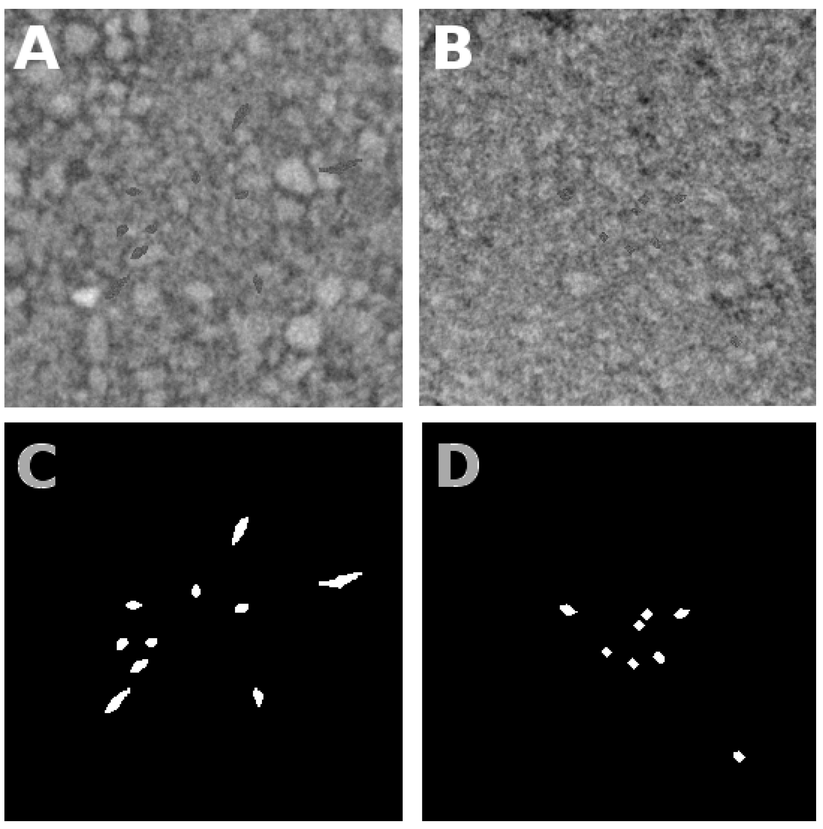
In this section, we designed a numerical experiment dedicated to the segmentation of simulated root systems after learning from other simulated root systems. The learning and testing images were both generated the same way: three-dimensional (244 × 244 × 26) pixels of real soil images with X-ray tomography. Root structure was generated from the L-system simulator of [30] under the form of [31] presented in 3D in [32]. Simulated roots were added to the soil by replacing soil pixels with root pixels. The intensities of the roots and the soil were measured from a manual segmentation in real tomography images of maize in Vulkasoil. The estimated mean and standard deviation are given in Table 1. We simulated the roots with a spatially independent and identically distributed Gaussian noise of fixed mean and standard deviation. As visible in Figure 2, learning and testing images do not have the same soil, nor the same root structure. This experiment is interesting because the use of simulated roots enabled us to experiment various levels of contrast between soil and root. Also, since the L-system used was a stochastic process, we had access to an unlimited sized training or testing data set. It is therefore possible with this simulation approach to investigate the sensitivity of the machine learning algorithm of the previous section to the choice of the parameters (size of the patch, size of the training data sets...).

4.1. Nominal Conditions

As nominal conditions for the root/soil contrast, we considered the first-order statistics (mean and standard deviation) of the roots and soil given in Table 1 which corresponded to the contrast found in the real acquisition conditions of maize in Vulkasoil (as described in the Material section. As visible in Figure 2A,B, these are conditions which provide very low contrast.
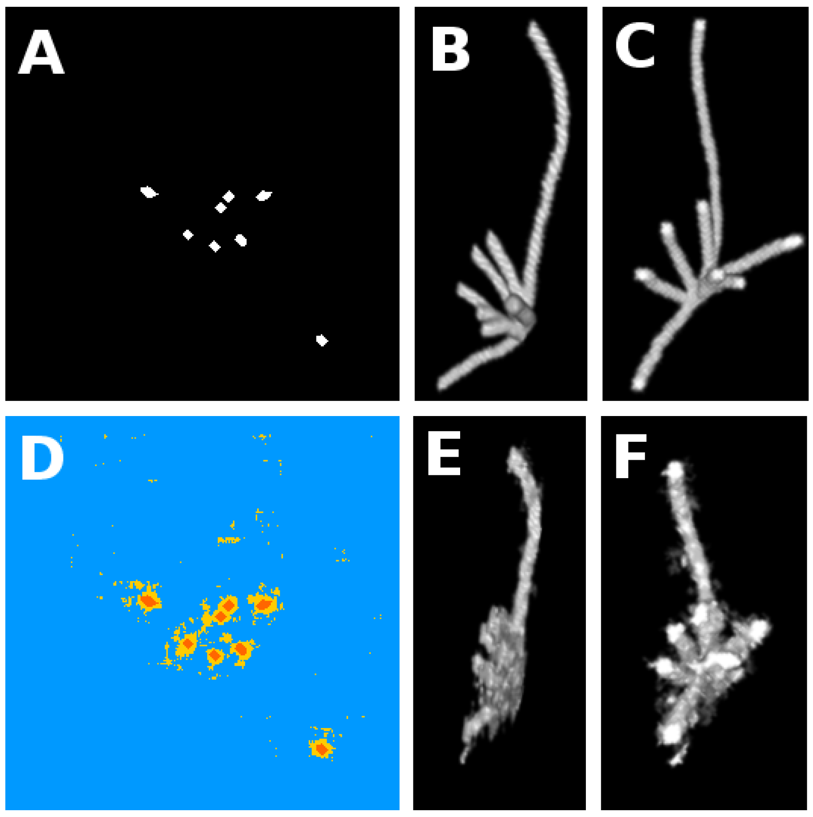
In the conditions of Table 1, with a combination of the information obtained with patches of 2 pixels and 15 pixels (see Section 4.2) and a training data set of 1000 patches, the segmentation performance obtained is given in Figure 3 with the confusion matrix in Table 2. To summarize the performance of the segmentation with a simple scalar, we propose a quality measure Q M obtained by multiplying sensitivity (which proportion of root pixels were detected as such) and specificity (which proportion of detected root pixels are truly root pixels)
Q M = T P 2 ( T P + F P ) ( T P + F N )
with T P being true positives, F P false positives, and F N false negatives. The quality measure Q M is maximized at 1 for perfect segmentation. For the segmentation of Figure 3, Q M = 0.23 . As visible in Table 2 and in Figure 3, the segmentation is not perfect, especially since false positives outnumber true positives. However, the quality of the segmentation cannot be fully captured by sole pixel to pixel average metrics. The spatial positions of false positive pixels are also very important. As visible in Figure 3, false positives (in yellow) are gathered just around the true positives and the small false positive clusters are much smaller than the roots. This means that we get a good idea of where the roots actually stand and with very basic image processing techniques such as particle analysis and morphological erosion, one could easily yield a much better segmentation result. Also, when the segmentation is applied on the whole 3D stack of images, it appears in Figure 3E,F, that the overall structure of the root system is well captured by comparison with the 3D structure of the ground truth shown in Figure 3B,C. It is useful to recall, while inspecting Figure 3E,F that the process classification is realized in a pixel by pixel two-dimensional (2D) process and it would also be possible to improve this result by considering 3D patches.
To obtain the three-dimensional (266 × 266 × 26 pixels) result of Figure 3E,F, about 2 h were necessary. The computing time was mainly due to the computation of the features (90%) on all the pixels of the testing image, while the other steps had negligible computation costs. Here, we considered the full feature space (1000 features) from [28]. It would certainly be possible to investigate the possibility of reducing the dimensions of this feature space while preserving the performance obtained in Figure 3. Instead, in this study we investigated the robustness of our segmentation algorithm when the parameters or datasets depart from the nominal conditions exhibited in this section.

4.2. Robustness

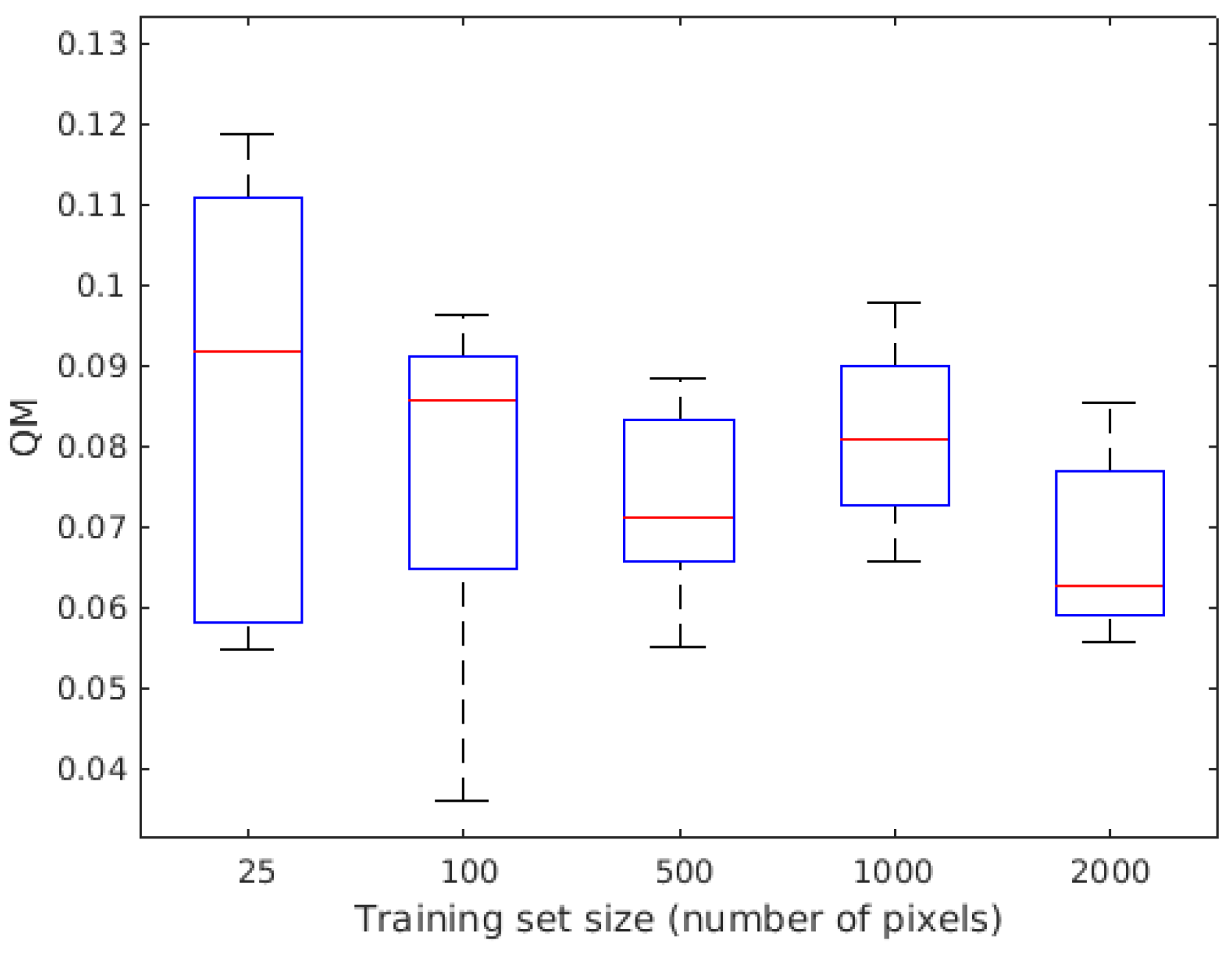
A first important parameter for using our machine learning approach is the size of the learning data set. In usual studies based only on real data of finite size, the influence of the learning data set is difficult to study since increasing the learning data set necessitates a reduced test data set. With the data from the previous section where roots are simulated, we do not have to cope with this limitation since we can generate an arbitrary large training data set. Figure 4 illustrates the quality of the segmentation obtained for different training data set sizes on a single soil–root realization. Degradation of the results is visible when decreasing the training size from 100 to 25 patches. As the root simulator is a stochastic process, the performance is also given in Figure 5 as a function of the size of the training data set in terms of box plot with average performance and standard deviation computed over five realizations for each training data set size tested. As visible in Figure 5, the average performance is almost constant, and the increase in the size of the training data set mainly provides benefits in terms of a decrease in the dispersion of the results.
A second parameter of importance to use our machine learning approach is the size of the patch. As visible in Figure 6 left, decreasing the size of the patch produces finer segmentation of the roots and their surrounding tissue but also increases spurious false detection far from the roots. Increasing the patch size (see Figure 6 right), produces a good segmentation of roots, with very few false detections far from the roots but with over-segmentation on the tissue directly surrounding the root. An interesting approach could consist in combining the results produced from a small and a large patch by a simple logical AND operation, i.e. an intersection, which detects as roots only the pixels detected as roots for both sizes of patches. This was the strategy adopted in Figure 3, which removes false detection far from the root while preserving the fine detection of the root with little false detection in the tissue surrounding the roots.

5. Segmentation on Real Roots

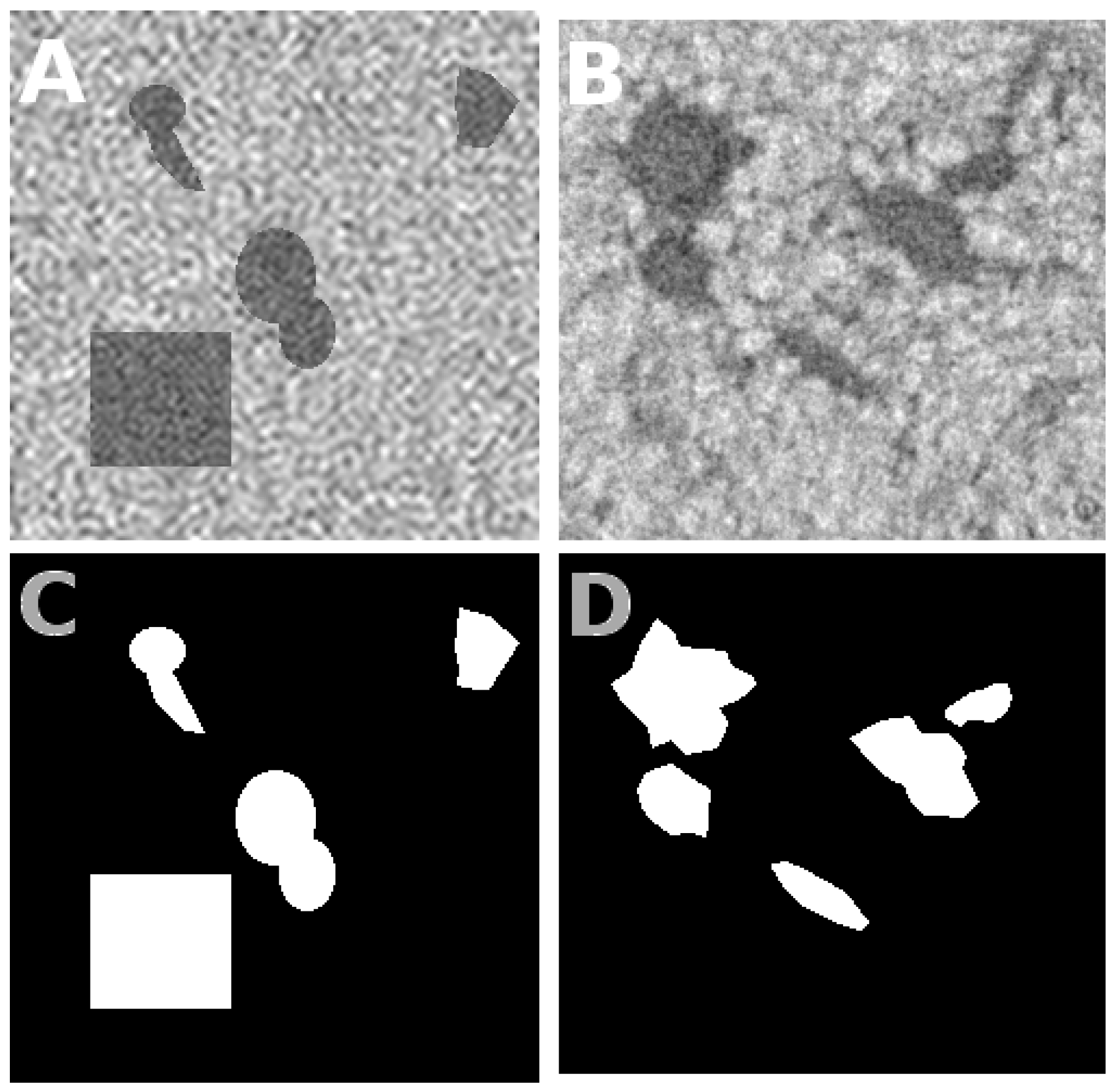
In this section, we investigate the performance of our machine learning algorithm when applied to real roots. The contrast considered is higher than in the previous section (see detail in Section 2) and corresponds to that found in [20]. We conducted the numerical experiment described in Figure 7 designed for the segmentation of real root systems after learning from simulated root systems and simulated soil.
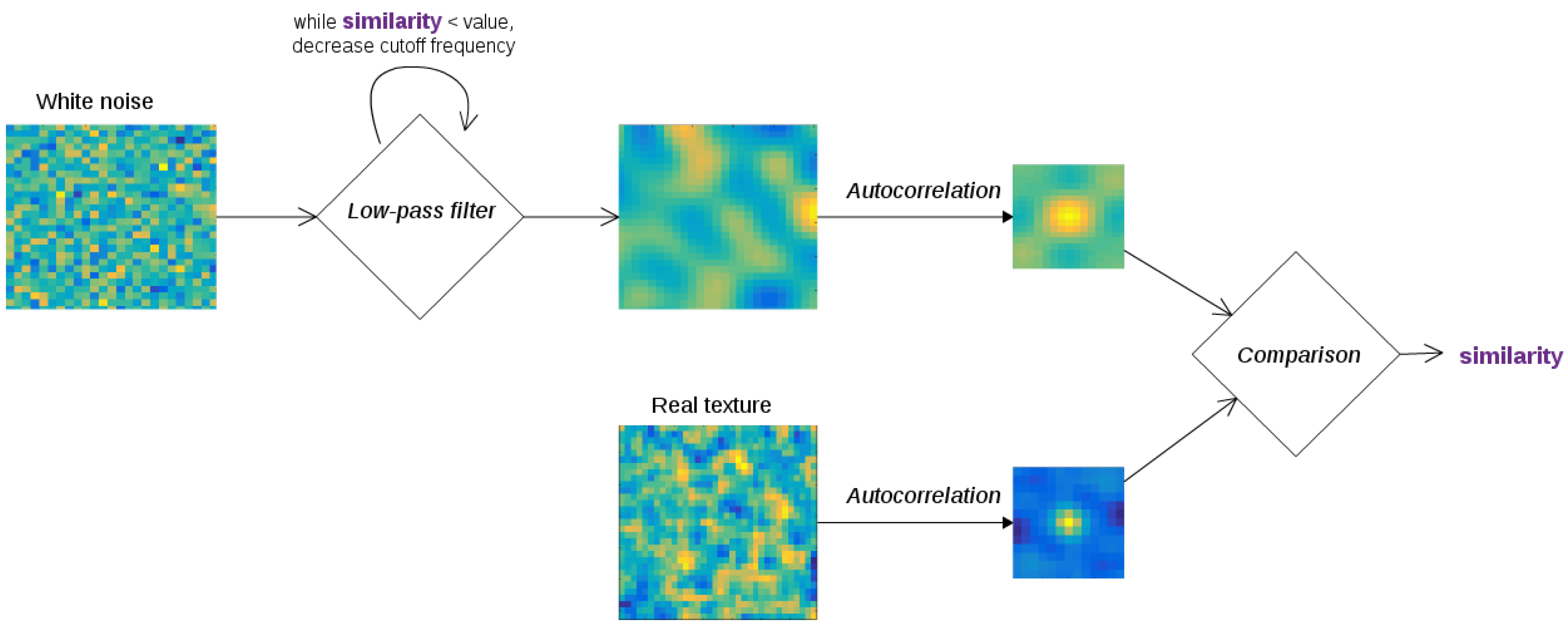
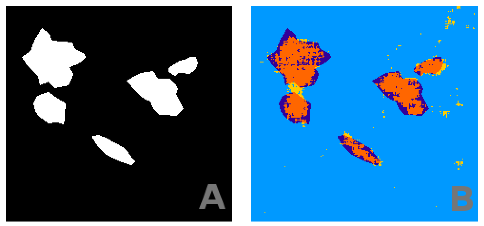
We tried to limit the size of the set of parameters controlling the simulated root and soil. First, the shape of the root systems is not chosen realistically, but the typical size of the object is chosen similar to the size of the real roots to be segmented. Also, as in the nominal conditions section, we tuned the first-order statistics (mean and standard deviation) of the roots and soil given in Table 3 which corresponded to the contrast found in real acquisition conditions (Figure 7B). In addition, we tuned the second-order statistics of the simulated soil on real data sets. These second-order statistics were controlled by means of the algorithm described in Figure 8. By operating this way, we obtained the fairly well-segmented images shown in Figure 9, with a confusion matrix given in Table 4.

5.1. Robustness

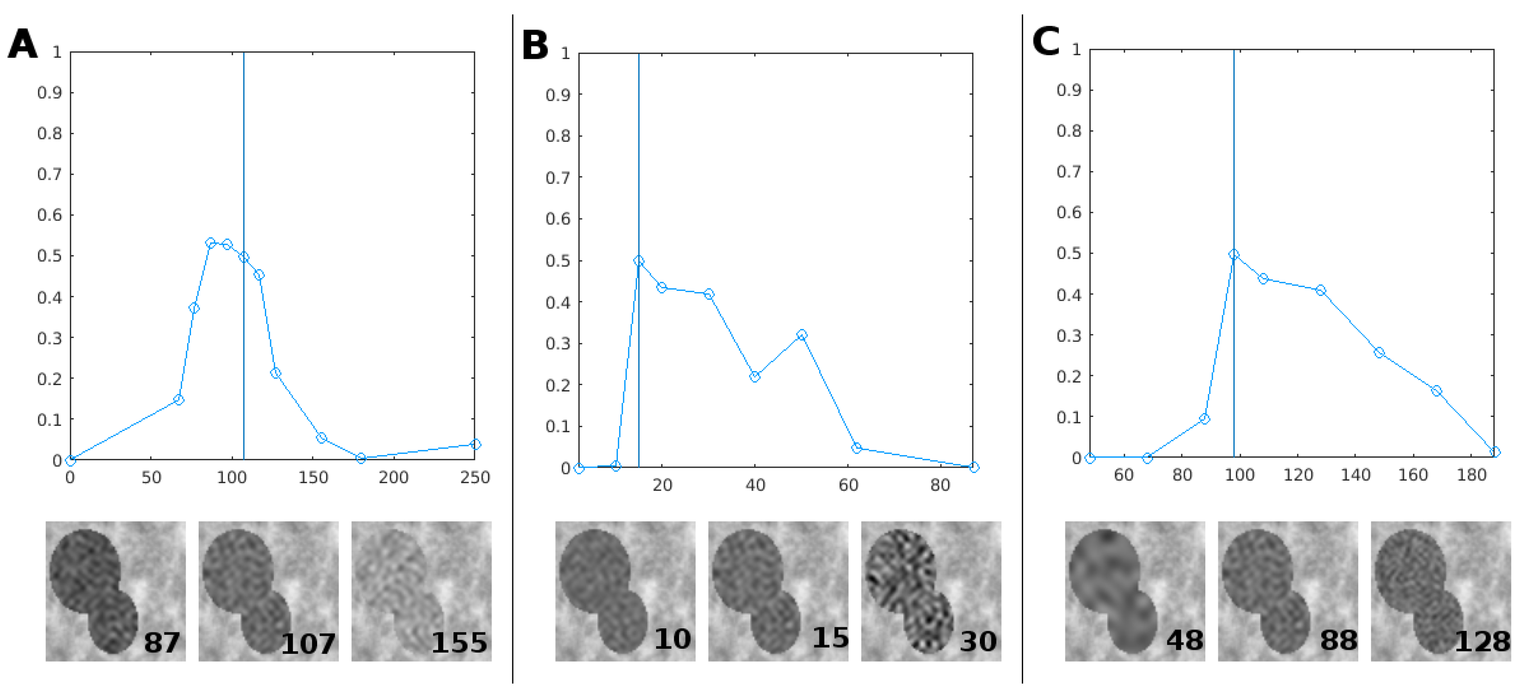
We have engineered the training data, generated from a simulation, to enable our machine learning algorithm to yield the good segmentation result of Figure 9. We found that the simulated training data must share some similar statistics with the real image for the segmentation to work. Specifically, it is sufficient to ensure the match of the first-order statistics (mean, standard deviation) and second-order statistics (autocorrelation) with the corresponding statistics of the image to be segmented. To test the robustness of this result, we have realized the same segmentation while changing one of these statistics in the training data, the other two staying similar to the testing data. Performance evolution can be found in Figure 10.
As expected, segmentation is best when the training data resembles testing data. However, segmentation remains good when statistics are spread in a reasonable range around the optimal value. These ranges are visible in Figure 10. For example, Figure 10A shows that the mean of the root in the 80–120 range provides reasonably good results compared to the optimum case of 97 which corresponds exactly to the mean of the image to be segmented. This establishes conditions where it is possible to automatically produce efficient segmentation of soil and roots in X-ray tomography. Also, if one expects the statistics of real images to depart from the those that served in the training stage, it would be possible to normalize the testing data at the scale of patches in order to maintain them in the range of the expected statistics.

6. Conclusions, Discussion and Perspectives

As a conclusion, in this article we have demonstrated the value of deep learning coupled to a statistical synthetic model to address the difficult problem of soil–root segmentation in X-ray tomography images. This was obtained from the so-called transfer learning approach where a convolutional neural network is trained on a huge image data set, distinct from the soil–root, for classification purposes to select a feature space which is then used to train an SVM on the soil–root segmentation problem. We demonstrated that such an approach gives good results on simulated roots and on real roots even when the soil–root contrast is very low. We have discussed the robustness of the obtained results with respect to the size of the training data sets and the size of the patch used to classify each pixel. We illustrated the possibility to perform segmentation of real roots from training on purely synthetic soil and roots. This was obtained in stationary conditions where both soil and root could be approximated by their first-order and second-order statistics.
As a point of discussion for the bioimaging community, one could wonder about the interest of the proposed approach coupling transfer learning and simulation when compared to more classical machine learning approaches. For instance, one could consider the random forest available under the WEKA 3D FIJI Plugin [33] and which produces a supervised pixel-based classification. On one hand, in contrast to what we propose with transfer learning, random forest features are not automatically designed but have to be selected by the user. A default mode for the user can be to select all features made available in a given implementation. However this mode is the most expensive in terms of computation time. An optimal selection of features can save time but requires an expertise which may not be accessible to all users. On the other hand, random forest is known to be efficient when small annotated data sets are available, while transfer learning requires a comparatively larger data set due to the higher number of parameters to be optimized. Beyond this comparison, it is important to underline that the use of simulated data in supervised machine learning is not limited to transfer learning and can be applied with any kind of classifier. It would thus be possible to train a random forest with synthetic data under WEKA 3D FIJI to benefit from the automated annotation.
Several perspectives are presented in this work. This use of deep learning for the soil–root segmentation problem can serve as a reference to investigate more complex situations which are found in practice. The water density of root may not be constant along the root systems. The soil, because of gravity, is often not found to present the same compactness along the vertical axis. It would therefore be important to push forward the investigation initiated in this article in the direction of non-stationarity of the gray levels in the root and in the soil. Also, one could add a physical simulator to include typical artifacts due to X-ray propagation in an heterogeneous granular material. As another direction of modeling improvement, one could consider enriching the L-system (as in [34]) to provide further biological insight.
As another direction, the deep learning algorithm considered for this article was purposely chosen as a basic reference from 2014 [28] which of course can be considered as outdated given the huge research activity with respect to testing network architecture. The computation time of our algorithm was rather long here due to the fact that the testing stage, where each patch was classified, was not parallelized. With a parallelization of this task the process could easily be reduced to few minutes. Also, it could be possible to use other neural network architectures, including the autoencoder approach [27], where the classifier produces the segmentation in a single pass. Better performance would thus for sure be accessible for the root/soil segmentation following the global approach described in this article.
Instead of focusing on solely efficiency, the goal of this article was rather to demonstrate the interest in coupling transfer learning with simulated data. As demonstrated in this article, the use of simulated data offers the possibility to generate unlimited data sets and enables the control of all parameters of the data set. It is especially useful to establish conditions for which transfer learning can be expected to give good results with real soil–root segmentation. Also, thanks again to the use of simulated data which creates annotated ground truth, our approach could serve to present a comparison with classic image analysis methods for soil–root segmentation (for instance [20]) or with other deep learning-based algorithms.

Author Contributions

Conceptualization, C.D. and D.R.; Methodology, D.R. and S.G.; Software, C.D. and R.S.; Validation, C.D., and R.S.; Formal Analysis, C.D. and D.R.; Investigation, C.D., R.S. and D.R.; Resources, D.R., S.G. and R.S.; Data Curation, R.S.; Writing-Original Draft Preparation, C.D., D.R., S.G. and C.F.; Writing-Review & Editing, D.R, S.G. and C.F.; Visualization, C.D.; Supervision, D.R. and S.G.; Project Administration, D.R. and S.G.; Funding Acquisition, D.R., R.S. and S.G.

Acknowledgments

This work received supports from the French Government supervised by the Agence Nationale de la Recherche in the framework of the program Investissements d’Avenir under reference ANR-11-BTBR-0007 (AKER program). Richard SCHIELEIN acknowledges support from the EU COST action ‘The quest for tolerant varieties: phenotyping at plant and cellular level (FA1306)’.

Conflicts of Interest

The authors declare no conflict of interest.

References

  1. Goodfellow, I.; Bengio, Y.; Courville, A.; Bengio, Y. Deep Learning; MIT Press: Cambridge, MA, USA, 2016; Volume 1. [Google Scholar]
  2. Ma, C.; Zhang, H.; Wang, X. Machine learning for Big Data analytics in plants. Trends Plant Sci. 2014, 19, 798–808. [Google Scholar] [CrossRef] [PubMed]
  3. Pound, M.P.; Atkinson, J.A.; Townsend, A.J.; Wilson, M.H.; Griffiths, M.; Jackson, A.S.; Bulat, A.; Tzimiropoulos, G.; Wells, D.M.; Murchie, E.H.; et al. Deep machine learning provides state-of-the-art performance in image-based plant phenotyping. GigaScience 2017, 6. [Google Scholar] [CrossRef] [PubMed]
  4. Kamilaris, A.; Prenafeta-Boldú, F.X. Deep learning in agriculture: A survey. Comput. Electron. Agric. 2018, 147, 70–90. [Google Scholar] [CrossRef]
  5. Mohanty, S.P.; Hughes, D.P.; Salathé, M. Using deep learning for image-based plant disease detection. Front. Plant Sci. 2016, 7, 1419. [Google Scholar] [CrossRef] [PubMed]
  6. Ubbens, J.R.; Stavness, I. Deep plant phenomics: A deep learning platform for complex plant phenotyping tasks. Front. Plant Sci. 2017, 8, 1190. [Google Scholar] [CrossRef] [PubMed]
  7. Condori, R.H.M.; Romualdo, L.M.; Bruno, O.M.; de Cerqueira Luz, P.H. Comparison between Traditional Texture Methods and Deep Learning Descriptors for Detection of Nitrogen Deficiency in Maize Crops. In Proceedings of the 2017 Workshop of Computer Vision (WVC), Natal, Brazil, 30 October–1 November 2017; pp. 7–12. [Google Scholar]
  8. Pawara, P.; Okafor, E.; Surinta, O.; Schomaker, L.; Wiering, M. Comparing Local Descriptors and Bags of Visual Words to Deep Convolutional Neural Networks for Plant Recognition. In Proceedings of the ICPRAM, Porto, Portugal, 24–26 February 2017; pp. 479–486. [Google Scholar]
  9. Mallat, S. A Wavelet Tour of Signal Processing; Academic Press: Cambridge, MA, USA, 1999. [Google Scholar]
  10. Yosinski, J.; Clune, J.; Bengio, Y.; Lipson, H. How transferable are features in deep neural networks? In Proceedings of the International Conference on Neural Information Processing Systems, Montreal, QC, Canada, 8–13 December 2014; pp. 3320–3328. [Google Scholar]
  11. Weiss, K.; Khoshgoftaar, T.M.; Wang, D. A survey of transfer learning. J. Big Data 2016, 3, 9. [Google Scholar] [CrossRef]
  12. Minervini, M.; Fischbach, A.; Scharr, H.; Tsaftaris, S. Finely-grained annotated datasets for image-based plant phenotyping. Pattern Recogn. Lett. 2015, 81, 80–89. [Google Scholar] [CrossRef]
  13. Scharr, H.; Pridmore, T.; Tsaftaris, S.A. Computer Vision Problems in Plant Phenotyping, CVPPP 2017: Introduction to the CVPPP 2017 Workshop Papers. In Proceedings of the 2017 IEEE International Conference on Computer Vision Workshop (ICCVW), Venice, Italy, 22–29 October 2017; pp. 2020–2021. [Google Scholar]
  14. Pawara, P.; Okafor, E.; Schomaker, L.; Wiering, M. Data Augmentation for Plant Classification. In International Conference on Advanced Concepts for Intelligent Vision Systems; Springer: Cham, Switzerland, 2017; pp. 615–626. [Google Scholar]
  15. Giuffrida, M.V.; Scharr, H.; Tsaftaris, S.A. ARIGAN: Synthetic arabidopsis plants using generative adversarial network. In Proceedings of the 2017 IEEE International Conference on Computer Vision Workshop (ICCVW), Venice, Italy, 22–29 October 2017; pp. 2064–2071. [Google Scholar]
  16. Ubbens, J.; Cieslak, M.; Prusinkiewicz, P.; Stavness, I. The use of plant models in deep learning: An application to leaf counting in rosette plants. Plant Methods 2018, 14, 6. [Google Scholar] [CrossRef] [PubMed]
  17. Barth, R.; IJsselmuiden, J.; Hemming, J.; Van Henten, E. Data synthesis methods for semantic segmentation in agriculture: A Capsicum annuum dataset. Comput. Electron. Agric. 2018, 144, 284–296. [Google Scholar] [CrossRef]
  18. Li, L.; Zhang, Q.; Huang, D. A review of imaging techniques for plant phenotyping. Sensors 2014, 14, 20078–20111. [Google Scholar] [CrossRef] [PubMed]
  19. Metzner, R.; Eggert, A.; van Dusschoten, D.; Pflugfelder, D.; Gerth, S.; Schurr, U.; Uhlmann, N.; Jahnke, S. Direct comparison of MRI and X-ray CT technologies for 3D imaging of root systems in soil: Potential and challenges for root trait quantification. Plant Methods 2015, 11. [Google Scholar] [CrossRef] [PubMed] [Green Version]
  20. Mairhofer, S.; Zappala, S.; Tracy, S.; Sturrock, C.; Bennett, M.; Mooney, S.; Pridmore, T. RooTrak: Automated recovery of three-dimensional plant root architecture in soil from X-ray microcomputed tomography images using visual tracking. Plant Physiol. 2012, 158, 561–569. [Google Scholar] [CrossRef] [PubMed]
  21. Pan, S.J.; Yang, Q. A survey on transfer learning. IEEE Trans. knowl. Data Eng. 2010, 22, 1345–1359. [Google Scholar] [CrossRef]
  22. Ruderman, D.L. Origins of scaling in natural images. Vis. Res. 1997, 37, 3385–3398. [Google Scholar] [CrossRef]
  23. Gousseau, Y.; Roueff, F. Modeling Occlusion and Scaling in Natural Images. SIAM J. Multiscale Model. Simul. 2007, 6, 105–134. [Google Scholar] [CrossRef]
  24. Chapeau-Blondeau, F.; Chauveau, J.; Rousseau, D.; Richard, P. Fractal structure in the color distribution of natural images. Chaos Solitons Fractals 2009, 42, 472–482. [Google Scholar] [CrossRef] [Green Version]
  25. Chauveau, J.; Rousseau, D.; Chapeau-Blondeau, F. Fractal capacity dimension of three-dimensional histogram from color images. Multidimens. Syst. Signal Process. 2010, 21, 197–211. [Google Scholar] [CrossRef] [Green Version]
  26. Chéné, Y.; Belin, E.; Rousseau, D.; Chapeau-Blondeau, F. Multiscale Analysis of Depth Images from Natural Scenes: Scaling in the Depth of the Woods. Chaos Solitons Fractals 2013, 54, 135–149. [Google Scholar] [CrossRef] [Green Version]
  27. Badrinarayanan, V.; Kendall, A.; Cipolla, R. Segnet: A deep convolutional encoder-decoder architecture for image segmentation. IEEE Trans. Pattern Anal. Mach. Intell. 2017, 39, 2481–2495. [Google Scholar] [CrossRef] [PubMed]
  28. Chatfield, K.; Simonyan, K.; Vedaldi, A.; Zisserman, A. Return of the Devil in the Details: Delving Deep into Convolutional Nets. In Proceedings of the British Machine Vision Conference, Nottingham, UK, 1–5 September 2014. [Google Scholar]
  29. Flandrin, P. Time-Frequency/Time-Scale Analysis; Academic Press: Cambridge, MA, USA, 1998; Volume 10. [Google Scholar]
  30. Leitner, D.; Klepsch, S.; Bodner, G.; Schnepf, A. A dynamic root system growth model based on L-Systems. Plant Soil 2010, 332, 171–192. [Google Scholar] [CrossRef]
  31. Benoit, L.; Rousseau, D.; Belin, E.; Demilly, D.; Chapeau-Blondeau, F. Simulation of image acquisition in machine vision dedicated to seedling elongation to validate image processing root segmentation algorithms. Comput. Electron. Agric. 2014, 104, 84–92. [Google Scholar] [CrossRef] [Green Version]
  32. Benoit, L.; Semaan, G.; Franconi, F.; Belin, E.; Chapeau-Blondeau, F.; Demilly, D.; Rousseau, D. On the evaluation of methods for the recovery of plant root systems from X-ray computed tomography images. In Proceedings of the Computer Vision-ECCV 2014 Workshops, Zurich, Switzerland, 6–7 and 12 September 2014; Volume 21, pp. 131–139. [Google Scholar]
  33. Arganda-Carreras, I.; Kaynig, V.; Rueden, C.; Eliceiri, K.W.; Schindelin, J.; Cardona, A.; Sebastian Seung, H. Trainable Weka Segmentation: A machine learning tool for microscopy pixel classification. Bioinformatics 2017, 33, 2424–2426. [Google Scholar] [CrossRef] [PubMed]
  34. Lobet, G.; Koevoets, I.T.; Noll, M.; Meyer, P.E.; Tocquin, P.; Pagès, L.; Périlleux, C. Using a structural root system model to evaluate and improve the accuracy of root image analysis pipelines. Front. Plant Sci. 2017, 8, 447. [Google Scholar] [CrossRef] [PubMed]
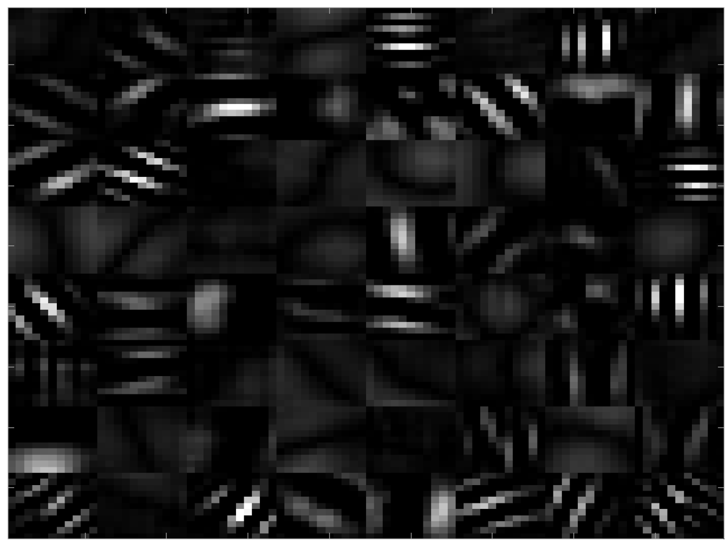
Figure 1. Convolutional filters selected by the first layer of the chosen convolutional neural network (CNN).
Jimaging 04 00065 g001
Figure 2. Presentation of simulated root systems. Panel (A) gives a slice of the training image (including soil and roots). Roots were generated by simulating an L-system structure and replacing soil pixels with root pixels, with gray intensity levels drawn from a white Gaussian probability density function with fixed mean and standard deviation. The positions of root pixels are shown in white in panel (C) which acts as a binary ground truth. Panel (B) gives a slice of the testing image where roots were generated the same way, and have the same mean and standard deviation as in panel (A). The ground truth of panel (B) is given in panel (D).
Jimaging 04 00065 g002
Figure 3. Experiments on simulated roots. Panel (A) gives a slice of the binary ground truth (position of the roots in white). Panels (B,C) provide a three-dimensional (3D) view of ground truth from two different standpoints. Panel (D) gives the result of the segmentation. Blue pixels signify true negative (soil pixels predicted as such), yellow represents false positive (soil pixels predicted as roots), orange signifies true positive (root pixels predicted as such), and purple shows false negative pixels (none in this result). Panels (E,F) are 3D views of the segmentation in the two viewing angles of panels (B,C).
Jimaging 04 00065 g003
Figure 4. Segmentation results for training sizes of 25, 100, 500, 1000, and 2000 patches, drawn using the 3D training image (see Figure 2). The image to segment measured 266 × 266, with 312 root pixels. The color code is the same as in Figure 3.
Jimaging 04 00065 g004
Figure 5. Quality of segmentation Q M for training sizes of 25, 100, 500, 1000, and 2000 patches. As the root simulator is a stochastic process, the performance is given in terms of a box plot with average performance (red line), standard deviation (solid line of the box), and max–min (the “mustach” of the box) computed over five realizations for each training data set size tested.
Jimaging 04 00065 g005
Figure 6. From left to right segmentation results for patch sizes 5, 15, 25, and 31 pixels wide. Roots in the image to segment could have a diameter of between 10 and 15 pixels. The color code is the same as in Figure 3.
Jimaging 04 00065 g006
Figure 7. Experiment on real roots: Panel (A) shows a slice of the training image (simulated). The corresponding binary ground truth is given in white in panel (C). Root intensity values are generated from a white Gaussian probability density function with a fixed mean and standard deviation, and are then low-pass filtered (see Figure 8) until the autocorrelation of the root is similar to that real roots. The same goes for the soil. Panel (B) is a slice of the testing image, a real image of X-ray tomography reconstruction. Panel (D) shows approximate ground truth of (B) created manually.
Jimaging 04 00065 g007
Figure 8. A pipeline for creating simulated texture with the same autocorrelation as real images. White noise is generated, then a low-pass filter is applied. This filter is a discrete cosine transform (DCT)->mask->DCT 1 transformation, where the size of the mask acts as the cutoff frequency of this filter. We start with a very high cutoff frequency (i.e., we do not change the white noise greatly). The autocorrelation matrix of the new image is then compared to that the real image, and the cutoff frequency is decreased if they are not similar enough, making the image “blurrier” and the autocorrelation spike wider.
Jimaging 04 00065 g008
Figure 9. Panel (A) shows ground truth (manually estimated). Panel (B) shows the segmentation obtained from our machine learning algorithm, with the parameters of training set size = 1000, patch = 12. The color code is the same as in Figure 3.
Jimaging 04 00065 g009
Figure 10. Panel (A), top, shows evolution of the quality metric Q M when the root intensity mean varies from 0 to 255 in the training data (s.d. and autocorrelation staying the same as testing data). The vertical blue line is the value of the root mean in the testing data (which we used for our results of Figure 9). The bottom part shows part of training images with different means as an illustration. Panels (B,C) show the same results for standard deviation and autocorrelation. Autocorrelation was quantified as the value of the cutoff frequency of the filter during the simulated image’s creation.
Jimaging 04 00065 g010
Table 1. Mean ( μ ) and standard deviation ( σ ) values for the roots and soil in Figure 2. Images are coded on 8 bits. Training and testing images have the same statistics.
StatisticsRoot μ Root σ Soil μ Soil σ
Values1001512520
Table 2. Confusion matrix of results in nominal conditions, as shown in Figure 3. The total number of pixels was 1,784,744.
Confusion MatrixRoot PixelSoil Pixel
Predicted root0.6%1.9%
Predicted soil 3 × 10 3 %97.5%
Table 3. Mean ( μ ) and standard deviation ( σ ) values for the roots and soil of the experiment with real root images. Training and testing images have the same statistics: simulated training images were created to resemble the testing ones.
ImageRoot μ Root σ Soil μ Soil σ
Statistics1101518025
Table 4. Confusion matrix of the results of Figure 9. Total number of pixels was 49.248 and the quality metric Q M = 0.57 .
Confusion MatrixRoot PixelSoil Pixel
Predicted root6.9%1.0%
Predicted soil3.7%88.4%