Abstract
The cold neutron imaging and diffraction instrument IMAT at the second target station of the pulsed neutron source ISIS is currently being commissioned and prepared for user operation. IMAT will enable white-beam neutron radiography and tomography. One of the benefits of operating on a pulsed source is to determine the neutron energy via a time of flight measurement, thus enabling energy-selective and energy-dispersive neutron imaging, for maximizing image contrasts between given materials and for mapping structure and microstructure properties. We survey the hardware and software components for data collection and image analysis on IMAT, and provide a step-by-step procedure for operating the instrument for energy-dispersive imaging using a two-phase metal test object as an example.
1. Introduction
In the last decade neutron imaging at pulsed neutron sources has been developed as an essential tool for materials science and engineering studies [1,2,3,4]. Time-of-flight (TOF) energy-dispersive neutron imaging at a pulsed source enables mapping of compositional and structural (phase, strain and texture) variations in metals [5,6,7] and imaging of phase transformations [8] with submillimeter spatial resolution. Moreover, spatial mapping of element compositions and remote temperatures via neutron resonance transmission analysis [9,10,11,12], and TOF imaging of magnetic fields [13] have been performed. Recently, 3D diffraction imaging via a TOF transmission technique has been verified [14], and the concept of mapping small angle scattering signals via wavelength-dispersive dark-field imaging has been demonstrated [15].
Most energy-dispersive imaging applications on TOF instruments are concerned with mapping structural parameters via Bragg edge analysis. Bragg diffraction removes neutrons from the incident beam, thus producing Bragg edges in the transmitted intensity as a function of wavelength. A Bragg edge transmission analysis can provide phase, strain and texture parameters of a material [16,17], and neutron radiography and tomography techniques can be employed to obtain 2D and 3D maps of those parameters. Bragg edge analysis works well with metals e.g., [18,19] but it has been applied for mapping mineral phases as well e.g., [20]. 3D reconstruction of elastic strains is being considered for systems under certain boundary conditions [21] whilst the ill-posed problem for strain tomography has been pointed out [22]. It should be noted that parallel to developments of Bragg edge analysis at pulsed sources, energy-resolved analysis at steady state sources is achieved by tuning the neutron energy using a double-crystal monochromator [23], allowing 2D and 3D mapping of structure parameters and phase transformations [24].
The fast development of TOF imaging is driven by the need for advanced materials research. In the past decade there have been significant developments in the design and installation of new imaging instruments on the one hand [2,25,26,27,28,29], and advances with detection systems on the other hand [30,31,32,33]. Accordingly, the available instruments and methods have made substantial progress since the early feasibility studies using a gated CCD camera [1]. Notably, two dedicated neutron imaging user facilities have been constructed at pulsed sources, namely RADEN [2] at J-PARC and IMAT [25,26,29] at ISIS. IMAT was installed on the 10 Hz pulsed source of the ISIS second target station at the Rutherford Appleton Laboratory, with substantial in-kind contributions from the Italian CNR. The beamline has recently seen cold and hot commissioning and is now being prepared for a user program. The instrument parameters have been determined [29], and the imaging cameras have been characterized [31,34,35].
Here we provide a first review of the instrument components used for TOF imaging on the new beamline, and we outline the set-up of the instrument as a user facility. The data collection and image analysis on IMAT is demonstrated using the same shrink-fitted Cu–Fe test object that was used in the earlier pilot study [1]. A detailed step-by-step guide includes the important aspects when performing a Bragg edge imaging experiment on IMAT. This paper complements the earlier description and characterization of the instrument for white-beam imaging [29].
2. TOF Imaging and Instrument Description
2.1. TOF Imaging
On a pulsed source energy-resolved imaging is enabled by a TOF analysis of the neutrons transmitted or scattered by the sample. This mode requires synchronization of the beamline components with the pulse generation, i.e., for choppers, monitors and cameras, using an external trigger signal which is provided by the source and marks the generation of neutrons in the target. For each pixel of a neutron camera the time of the neutron arrival relative to this trigger is measured. The wavelengths of the detected neutrons are calculated from their time of flight by
where λ is the neutron wavelength (in Angstrom), h is Planck’s constant, T is the neutron time of flight (in seconds), ∆T0 is the time offset of the source trigger received by the data processing electronics (in seconds), m is the neutron mass, and L is the flight path from source to camera (in meters).
An overview of the TOF imaging set-up and the signal processing for an energy-dispersive measurement on IMAT is shown in Figure 1. At the heart of this figure are the sample and the pixel detector, here for the example of the GP2 detector [30,31]. The detector is placed at a known distance from the source. On IMAT, a neutron pulse is generated and moderated every 100 ms, and the flight path to the camera is about 56 m. The wavelength dispersion of the incoming pulses is illustrated by the different colors of the neutrons, with the higher energy (red) neutrons arriving earlier in the camera than the low energy (blue) neutrons. The energy dependence of the beam attenuation of the incoming neutron pulses is reflected by the ‘color-dependent’ reduction of neutrons as they transverse the sample. In the camera, each neutron is individually and uniquely tagged in position and time within each neutron pulse.
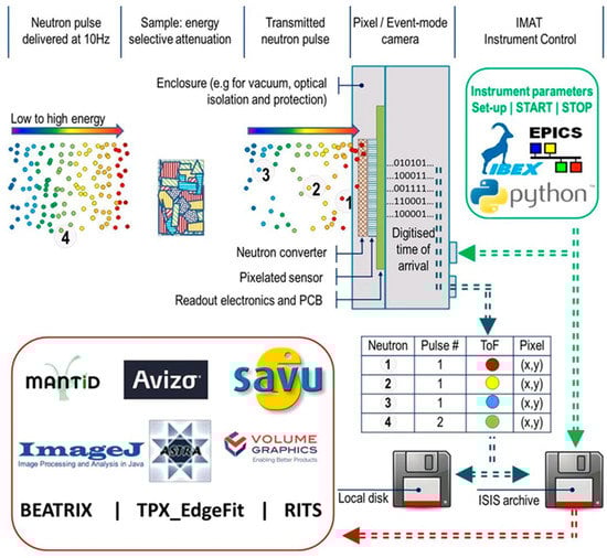
Figure 1.
Time-of-flight (TOF) imaging schematic. The sketch illustrates the energy-dependent beam attenuation, as measured in a TOF imaging experiment. The TOF pixel detector records every neutron’s arrival time, with its (x,y) position. Four neutrons, labeled 1–4, from two separate neutron pulses are labelled to illustrate and emphasize this point. The camera is controlled via the IBEX GUI used on IMAT. For the image analysis a range of tools is available.
The imaging camera (or pixel detector) is operated via the IBEX [36] instrument control program which is based on the EPICS [37,38] software tools and libraries. The registered neutrons are stored as images or event lists, and treated with a toolbox of image analysis packages. A typical raw data size for a white-beam radiography and an energy-dispersive radiography is 8 Mbyte and 1.5 GByte, respectively. An event-mode generated energy-dispersive data set for 10 k pixels and 4000 k time bins is of the order of 5 GByte per hour. For the size of a tomography data set these numbers are to be multiplied by the number of projections.
There are two important parameters to be considered when defining the performance of a time-of-flight imaging instrument: (i) The maximum value of the wavelength band; (ii) the wavelength resolution. The maximum wavelength band is defined by the need to avoid frame overlap, i.e., the superposition of neutrons coming from different neutron pulses into the same time frame. The wavelength band width is given by:
where f is the repetition rate, and L is the flight path from source to pixel detector. The repetition rate is usually the pulse frequency of neutron source, but can be set to values lower than the source frequency using neutron choppers by suppressing pulses from the source. For a flight path of 56 m and a frequency of 10 Hz the wavelength band width is about 7 Å. With the suppression of every other pulse by a chopper system the effective pulse frequency is 5 Hz, and the band width is about 14 Å. The accessible maximum wavelength range defines which energy-dependent features, e.g., Bragg edges, are observed in one acquisition.
The wavelength resolution of the instrument is determined by the uncertainty δλ to which a given wavelength can be determined. The actual width and shape of the neutron pulse for a particular wavelength, and its dependence on wavelength, are complex functions dictated by the type, geometry and physical processes occurring within the moderator. For a given wavelength, the relative uncertainty δλ/λ determines the broadening of a feature, e.g., a Bragg edge, in a TOF spectrum. The resolution function for IMAT has been determined recently [29].
In summary, on a TOF instrument energy-resolving or wavelength-discriminating measurements are performed in a straightforward way, allowing for monochromatic, energy-selective and energy-dispersive neutron imaging, in addition to ‘white-beam’ and ‘pink-beam’ (narrow wavelength range) imaging applications. The hardware and electronic time resolutions of TOF cameras and detectors are often much better than the intrinsic instrument resolution. With this in mind, we use the term ‘energy-selective neutron imaging’ if neutron radiographies are collected for one or more, wide or narrow, wavelength bands. Selecting certain wavelength bands is useful, for example, for enhancing contrasts by exploiting the variation of the attenuation with energy, be it for different materials or for different phases of the same material. ‘Monochromatic neutron imaging’ is a special case of energy-selective imaging if one narrow energy channel is selected. Furthermore, energy-selection is a prerequisite for ‘energy-dispersive neutron imaging’ where histogramming or scanning within a wavelength range is performed with a sufficiently fine bin-width, for example across a Bragg edge of a material.
2.2. IMAT Instrument
2.2.1. Source and Choppers
IMAT [25,26] is a cold-neutron imaging facility installed on the ISIS second target station TS2, a low-power 10 Hz pulsed source of about 50 kW. The length of the beamline from source to sample position is 56 m. Figure 2 shows design drawings of the full length of the instrument and a detailed depiction of the sample area. Further illustrations of the instrument set-up are provided in Figure 3. Neutrons at ISIS are produced by spallation reactions induced by high-energy protons impinging on a tungsten target. IMAT is installed on the coupled 18 K hydrogen moderator on beamport W5. The neutrons exiting the moderator are transported by a straight, m = 3, evacuated supermirror guide to the sample area. A 20 Hz T0 chopper at 12.75 m from the moderator serves as fast neutron and gamma filter. Two 10 Hz double-disk choppers (at 12.2 m and 20.4 m) are used to define wider (e.g., 6 Å) or narrower (e.g., 1 Å) wavelength bands but also to prevent frame-overlap of neutrons between successive time frames.
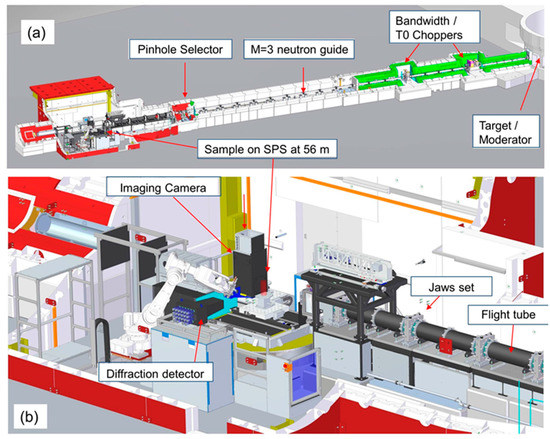
Figure 2.
IMAT instrument layout. (a) The length of the instrument from source to sample position is 56 m. (b) The main components in the sample area are: evacuated flight tubes; beam limiting jaws; sample positioning system (SPS); imaging camera; diffraction prototype detector.
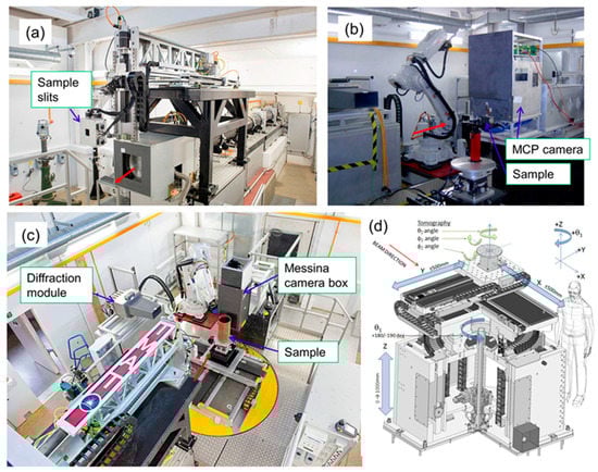
Figure 3.
Installation of IMAT on TS2. (a) upstream view from the sample point showing flight tubes and sample slits (out of beam) inside the blockhouse; (b) MCP detector setup; (c) sample area view through the open roof into the IMAT blockhouse, with the Messina camera box carried by a robotic arm; (d) concept drawing of the sample positioning system (SPS).
2.2.2. Beamline Components
The neutron guide ends just upstream of a pinhole selector at 46 m. The pinhole produces a quasi-parallel neutron beam adopting a specific divergence (or L/D) value, where D is the diameter of the aperture and L is the distance to the neutron camera. However, it should be noted that the L/D value is affected by both the divergence characteristic of the guide and the pinhole geometry [29]. The remote-controllable pinhole selector wheel offers a choice of five circular apertures, to define different L/D ratios between 125 and 2000, and one large square aperture of 100 × 100 mm2. The selector uses a system of changeable cartridges into which neutron-absorbing sheets (typically consisting of boron based materials) with circular or rectangular apertures are inserted. Between the end of the supermirror guide at 45.7 m and the pinhole selector a filter or diffuser can be inserted into the beam if required. The purpose of a beam diffuser is to wash out spatial inhomogeneities in the neutron beam which are present mostly due to the finite moderator size and gaps in the neutron guide for choppers, monitors and vacuum valves. A non-hydrogenous, small angle scattering material is considered as diffuser. A graphite diffuser is currently being evaluated for IMAT; so far, the filter cartridge was kept empty.
From the pinhole the neutrons travel through approximately 9 m of evacuated flight tubes of 320 mm diameter (Figure 3a), before reaching the nominal sample position at 10 m from the pinhole selector. An pneumatically-driven attenuator (‘fast shutter’) made of an 10B-coated Al-sheet is installed upstream from the sample position as neutron absorbing blade that is driven into the beam to reduce flux on the sample, thereby minimizing sample and camera activation when data is not being taken.
Four diagnostic TOF 40μ-vanadium-foil beam monitors are installed along the beamline, at 11.7 m (M1), 19.8 (M2), 20.9 m (M3), and 46.2 m (M4) from the moderator, to inform about the status of the incident beam. M1 to M3 are positioned before and after the choppers; M4 is positioned directly after the pinhole. A fifth, retractable monitor (M5) with a thickness of 100 μm of the vanadium foil installed at 49.0 m will be used for normalization of diffraction data. This monitor is usually driven out of the beam for imaging experiments. An additional, portable TOF neutron beam monitor is available for characterization of the beam spectrum at the sample position. The latter monitor uses a 6Li-based GS1 glass scintillator (7Li-2.4%wt6Li) with an active volume of 0.95 × 0.96 × 0.95 mm3. The monitor is calibrated against measured and Monte Carlo simulated scattering data.
The IMAT beam size can be varied between 1 × 1 mm2 and 200 × 200 mm2 using five sets of ‘jaws’ each made of four blades of 10 mm thick sintered boron-carbide. A set of retractable sample slits (using four 3 mm thick 10B blades and with adjustment options along the beam direction) can be used to define a small aperture between 1 × 1 mm2 and 50 × 50 mm2. As such, the slit set produces a well-defined beam size just in front of the sample. The sample slit system and its support frame can be seen in Figure 3a.
The IMAT sample positioning system (SPS) with its reference at 56 m from the source is used for sample alignment, and for sample rotation for tomography experiments. The SPS has seven axes for sample movements: a large rotation (Θ1; range: 360 degrees), three linear stages (‘X’, ’Y’, ‘Z’; ranges: 1 m), two orthogonal tilts (φ1, φ2; range 10 degrees), a tomography rotation stage (Θ2, range: 360 degrees). The x, y, and z directions of the SPS in their home positions are in beam direction, transverse direction and vertical direction, respectively, consistent with the coordinate system of IMAT. A concept design drawing of the SPS is given in Figure 3d. The SPS is designed to lift and accurately position 1.5 t loads. The tomography rotation stage can carry smaller samples <50 kg; the stage can be dismounted if required. For sample alignment a laser beam along the incident neutron beam and two theodolites are available.
A detailed description of the instrument and its measured performance has been given recently [25,26,29]. It should be noted that IMAT is about to be equipped with additional diffraction detectors, for strain and texture analysis via neutron diffraction. A prototype diffraction module is shown in Figure 2b and Figure 3c.
2.2.3. IMAT Cameras
Three camera systems are available on IMAT, including two TOF pixel detectors. TOF pixel detectors with high spatial and high timing resolution are essential for performing energy-dispersive measurements on a pulsed-source instrument like IMAT. The currently available cameras and detectors are listed in Table 1 with their main parameters.

Table 1.
Current IMAT camera options.
A microchannel plate detector (MCP) developed by the University of California at Berkeley [32] utilizes neutron absorption by boron and gadolinium atoms impregnated into the MCP glass followed by the generation of secondary electrons and signal amplification within the pores of the MCP localized to a ~10 μm area. The field of view of the detector is 28 × 28 mm2 and the detector is capable of providing a TOF spectrum for each pixel of the 2 × 2 array of Timepix readout chips (512 × 512 pixels, each 55 × 55 μm2). The fast electronics with 320 μs readout time enables acquisition of multiple ‘shutters’ (maximum 1200) for each neutron pulse with individually controlled time resolution within each shutter. It can be noted that a ‘shutter’ is synonymous with a ‘TOF range’ within the time frame between two source pulses. The distance between the neutron-sensitive MCP and the front of the aluminium window of the detector box is 12 mm.
An active pixel sensor (GP2) uses the PImMS-2 CMOS [30,31]. A gadolinium sheet is used for converting neutrons to electrons which are then counted by a CMOS sensor with a pixel size of 70 μm. A number of up to 4096 times slices can be used; the timing resolution is better than 12 ns. The GP2 has four 12-bit registers per pixel which reduces the effect of saturation (or event overlap). Due to its compact design the camera can be placed close to a sample or sample environment where a small sample-detector distance is required.
The Messina optical camera box of IMAT uses a scintillator screen for neutron-to-light conversion, a 45 degree mirror, a lens to focus the light on a digital CCD or CMOS camera chip. The field-of-view ranges between 60 × 60 and 211 × 211 mm2. The system is used for white-beam radiography and tomography measurements as well as for energy-selective applications for contrast enhancement and contrast variation, and potentially for large-field-of-view Bragg edge mapping. A range of scintillators, either ZnS/6Li or Gd2O2S (Gadox), of different thicknesses are available. The field of view and the spatial resolution can be adapted by changing the lens. With a 2 k × 2 k pixel camera the best spatial resolution is achieved for a field of view of 60 × 60 mm2. It is worth mentioning that the camera has a built-in optical autofocus system [34]. Different CCD/CMOS camera modules can be mounted on the box.
The IMAT cameras can be interchanged during a user experiment, and calibrated in less than two hours. A camera support frame, with the position adjustable along the beam direction, and a 7 axis robotic manipulator arm are available to support a camera when in use. The robotic arm solution was selected based on the requirement to place and remove multiple detectors in the sample area above the SPS; it allows for maximum flexibility to accommodate future detector designs.
There will be continuous upgrades and developments of imaging cameras on IMAT, especially with regards to the active sensitive areas and the neutron detection efficiencies. Limiting factors for energy-selective measurements for the CCD and CMOS systems are the minimum field of view (limits spatial resolution) and the thickness of the scintillation screen (related to a blurring of the event determination; limits spatial resolution) and the afterglow and activation of the screens (limiting the time-of-flight determination from tens of microseconds to seconds). For IMAT a timing resolution of at least 20 microseconds is required for TOF applications. Both IMAT pixel detectors MCP and the GP2 have a potential for the active areas to be increased by tiling, i.e., by placing readout chips side by side. For instance, the current generation of the Timepix chip is three-side buttable allowing 28 × N mm configurations. Future chips will be four-side buttable by implementation of through-silicon vias. Envisaged development lines for neutron imaging cameras and detectors on IMAT are listed in Table 2.
Table 2.
Envisaged future IMAT camera systems.
2.3. IMAT Spectrum and Energy-Selection
The ‘natural’ (non-overlapping) neutron bandwidth of IMAT is 7 Å, according to Equation (2), for a source frequency of 10 Hz and a flight path of 56 m. Due to the finite opening and closing times of the 10 Hz choppers of about 3 ms, the effective bandwidth is smaller, and close to 6 Å. Figure 4 displays a single-frame IMAT spectrum (blue curve) for 10 Hz operation of the choppers, and with the choppers opening with the pulse generation. The data were collected with the monitor M5 at 49 m from the source. The wavelength band can be shifted upwards the wavelength scale at will, by dephasing the chopper openings. For the standard IMAT experiment a range from 1 to 7 Å is usually adequate. The choppers can be run at half frequency to access the second frame, thereby doubling the effective neutron wavelength bandwidth to 12 Å (black curve in Figure 4). In this case, every other neutron pulse is removed by the choppers, hence the intensity drops by a factor of about 2. The pink curve in Figure 4 demonstrates selection of a narrow bandwidth of about 0.63 Å (FWHM) near the maximum of the flux distribution at 2.6 Å. A bandwidth selection is of interest, for example, for producing neutron images beyond the Bragg cut-off wavelength where attenuation is dominated by absorption and where crystal structure and crystal grain effects on the images are minimized. A narrow band is also used to minimize the errors being made by averaging measured attenuation coefficients in the presence of spectral beam inhomogeneities across the field of view and/or beam hardening effects for highly absorbing materials.
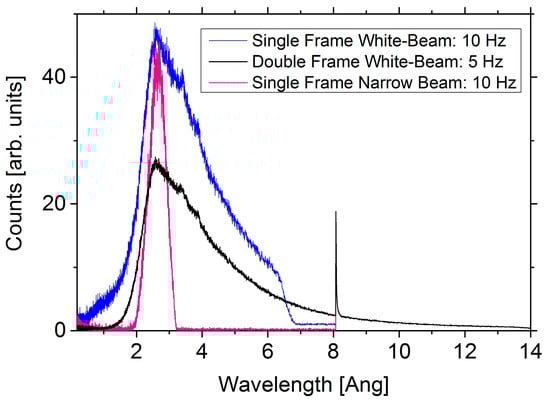
Figure 4.
Beam spectra for different chopper settings, not corrected for efficiency: single-frame white-beam; narrow-bandwidth (pink) beam; double frame white-beam. The spike at 8.1 Å is the gamma pulse originating when the protons hit the target, in the absence of the T0 chopper. Data were collected in histogram mode for neutron counts as a function of the neutron time-of-flight with a logarithmic time bin of ΔT/T = 0.001 in a range between 5 μs to 100 ms and 5 μs to 200 ms for single-frame and double frame acquisitions, respectively.
2.4. Instrument Parameters
Table 3 reviews some of the IMAT instrument and performance parameters, which were in part determined during a recent scientific commissioning period [29]. Estimated values of spatial resolutions and collections times on IMAT are given in the lower part of the table, for an L/D of 250. For Bragg edge imaging, the spatial resolution is not limited by the pixel size (e.g., 55 μm corresponding to a spatial resolution of 110 μm) but rather by the available neutrons per space-time pixel, and by the beam divergence and associated image blurring. Therefore, for IMAT experiments pixel events are almost always combined in a macro-pixel. Moreover, Bragg edge imaging requires sample thicknesses of several millimeters for obtaining significantly pronounced Bragg edge features. For example, for a 25 mm thick sample and for L/D = 250 the image blurring is 25/250 = 0.1 mm. It is obvious that collection times depend on the type of material studied, i.e., on neutron scattering lengths and structure factors.
Table 3.
IMAT instrument parameters for TOF imaging. Performance parameters are taken from [29]. Estimated resolution and counting times refer to radiography (2D) and tomography (3D) experiments.
2.5. Infrastructure and Software
IMAT was designed and built in a way that an inexperienced user is able to operate most components safely and efficiently. Like all ISIS instruments IMAT include safety features such as a personal protection system for safe access of the experimental area, as well as an advanced motion control safety system. Most operations on IMAT can be performed remotely via a central control station (called NDXIMAT) in the IMAT cabin. A plan view of the IMAT extension building in Figure 5 indicates some of the main IMAT infrastructure points around the shielded experimental area (‘IMAT blockhouse’):
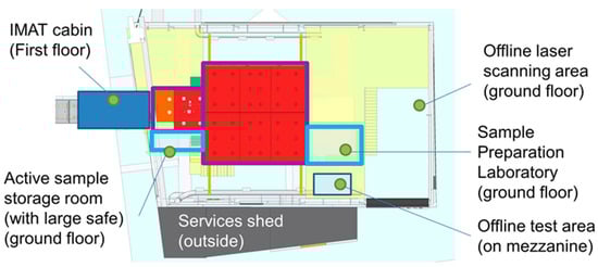
Figure 5.
Plan-view sketch of the IMAT extension building, showing the infrastructure around the IMAT blockhouse.
- IMAT cabin: With work stations for instrument control and image analysis, and links to the ISIS data archive;
- a small chemistry/sample preparation laboratory;
- a large safe in lockable room for storing large samples, and valuable samples and objects. The room can be used for sample storage before and after irradiation, i.e., for radio-activated samples and equipment;
- an offline-testing area for sample environment, in particular for mechanical loading rigs;
- a hydraulic system to deliver 210 bar hydraulic pressure at 90 lpm flow rate to two manifold stations - one positioned at the sample area and another station at the offline-testing area.
- a services shed outside the IMAT extension for hydraulic pumps, He gas compressors for cold heads, vacuum pumps;
- an offline laser scanning area
A 2-ton crane is available to load samples and equipment into the sample area through a power-operated roof.
Figure 6 gives an overview of the data management structure. The IBEX instrument control graphical user interface [36] runs on the NDXIMAT machine from which all instrument components, choppers, pinhole rotator, beam monitors, fast attenuator, jaws, slits, imaging cameras and sample environment are controlled. IBEX has also control of the ISIS DAE-2 data acquisition system which manages the ISIS trigger signals, records the monitor counts as a function of time of flight, and in future will readout the IMAT diffraction detectors. Figure 7 shows a screenshot of the IBEX GUI. The control of components are achieved via EPICS operator interfaces [38] but, most importantly, via command line and python scripts which enables scripting of most instrument control options.
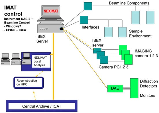
Figure 6.
IMAT data management structure.
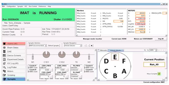
Figure 7.
IBEX Graphical User Interface: IMAT instrument and camera control.
A camera/pixel detector is set-up on a dedicated camera PC, usually with its own camera GUI for stand-alone operations, for example PIXELMAN [40] in the case of the MCP, and the Messina GUI in case of the optical camera box. Remote and scripted control of the camera interface is achieved via EPICS. The image formats currently implemented are: TIF or FITS for single images; stacks of FITS for the MCP; event lists for the GP2. The filename of a single image, or the name of an image stack (for a number of rotations for tomography; a number of time bins for the MCP/GP2) has a unique run number prefix. It is envisaged that in the medium term the IMAT data will be saved and archived in NeXus [41,42] format.
Software tools for image analysis and Bragg edge mapping include BEATRIX [43], TPX_EdgeFit [44] and RITS [45]. A number of pilot projects have highlighted that IMAT needs flexible and adaptable software for the analysis of energy-dispersive data, as the analysis requirements for experiments vary. Packages for 3D reconstruction (Octopus [46]; Tomopy [47]; AstraToolbox [48]) and segmentation and volume rendering (VgStudioMax [49], Avizo [50]) of white-beam data are available for users on IMAT. Remote access to software for users will be implemented in the near future. A python-based interface for pre-processing raw images and for preparing images for various reconstruction packages is being developed within the MANTID [51] software framework. The analysis is performed either on local desktop workstations or multi-core CPU/GPU high performance clusters (HPC). In addition, efforts are made to process IMAT data with the SAVU [52,53] reconstruction pipeline. Currently, IMAT data are processed / reconstructed locally, partially using licensed packages. In the medium term, complete processing and reconstruction will be performed with freeware tools, so that users can analyze data at their home institutions. It is envisaged that HPC clusters will be required for particularly computational intensive iterative codes.
3. Demonstration of Bragg Edge Analysis on IMAT
Here we present a step-by-step description of an energy-dispersive imaging experiment on IMAT. Data collected with the MCP detector on a shrink-fitted Fe–Cu test object are used to demonstrate the data collection and image analysis procedures. The aim of the measurement on the test sample is to determine the crystalline phase and axial strain distributions of the iron and copper phases with a resolution of 200 μm.
3.1. Sample Description
The test object consisted of a solid copper cylinder of 10 mm diameter and 25 mm height shrink-fitted into a hollow ferritic iron steel cylinder of the same height but of 25 mm outer diameter with a small interference fit at the inner diameter. The shrink-fitting was achieved by cooling the copper cylinder in liquid nitrogen whilst heating the hollow iron cylinder on a hot-plate [54]. The temperature difference and extent of misfit were sufficient to allow an easy shrink-fitting of the copper cylinder into the bore. A photo and schematic of the sample is shown in Figure 10a.
3.2. Flight Path Calibration
The camera is installed in the beam path using a robotic arm, with a reproducibility of better than a millimeter. For accurate lattice spacing measurements, i.e., for strain mapping, and for studying phase transitions of crystalline samples, it is recommended that a standard sample is measured and the flight path calibrated, especially if the camera was reinstalled or moved between measurements. This will also ensure that the camera is working as expected. The flight path is determined from several Bragg edge positions using the neutron time of flight relation of Equation (1). A beryllium sample was selected for calibration because it yields a spectrum of well separated and well-defined Bragg edges in a relatively short time. Other samples for calibration used on IMAT are iron and ceria (CeO2) powders. Figure 8a shows the Bragg edge spectrum of the beryllium sample, contained in an aluminium box, measured for about 30 min and averaged over the whole sensitive area of the MCP detector. The thickness of the Be-sample along the beam direction was 80 mm. For the flight path calibration the fitted TOF Bragg edge positions for different lattice planes (hkl) are plotted against tabulated beryllium d-spacings (and hence wavelengths) (Figure 8b). Linear regression of calibration points yields the flight path L and ∆T as fitting parameters: L = 56.35 ± 0.05 m and ΔT0 = 1.35 ± 35 us.
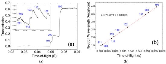
Figure 8.
TOF flight path calibration using a beryllium sample. (a) Indexed TOF spectrum for a large region of interest of the sample; (b) plot of the nominal Be Bragg edge positions versus measured Bragg edge positions. The slope yields the flight path; the intercept yields the TOF offset, according to Equation (1).
3.3. Data Collection
3.3.1. Sample Alignment and Camera Preparation
The sample was installed in front of the Al window of the MCP detector, with the neutron beam along the cylinder axis of the sample. In this way the Bragg edge shifts correspond to the axial strain components of the Fe and Cu sample components. The sample was mounted on a boron carbide pedestal to reduce scattering of neutrons, considering that the neutron beam is larger than the sample. The distance between the downstream end of the sample and the active sensor is 20 mm, including a 12 mm distance between the front of the Al window, a 5 mm thick boron carbide B4C neutron shielding plate on the front face of the MCP, and a distance of 3 mm of the sample to the B4C shielding face. The following settings were made, in preparation of the measurements:
- -
- The IMAT disk choppers were set to 10 Hz, and dephased by 20 ms to define a TOF range of 32–115 ms, corresponding to a wavelength band of about 2.2–8 Å. The same delay of 20 ms was set for the MCP detector (to be added to the TOFmin and TOFmax values in Table 4). The MCP system used a 10 Hz trigger signal from the choppers.
Table 4. Expected Bragg edge positions of Cu and Fe; lower and higher TOF boundaries of MCP shutters (in seconds) indicating the readout gaps, and spanning a total range 12–95 ms. In addition, the trigger signals and acquisition frame are delayed by 20 ms; MCP clock frequency 100 MHz/2n with clock divider (n); time channel width (in μs); number of time bins (sum: 2612).
- -
- The beam size was set to 35 × 35 mm2 to fully illuminate the MCP active sensor.
- -
- The pinhole was set to 40 mm diameter; i.e., the L/D was 245 [29]; the part of the sample furthest away (45 mm) from the sensor determines the best resolution of 45/245 = 180 μm.
- -
- The expected positions of Bragg edges can be found in crystallographic databases. There are tools available to calculate Bragg edge spectra taking the structure information, and neutron absorption and neutron scattering cross sections into account e.g., [55].
- -
- The TOF ranges and the time bins were set in the MCP detector interface (by editing ShutterValues.txt). Three MCP readouts were chosen between 32 and 115 ms, to reduce event overlap (see below) whilst avoiding having Fe and Cu Bragg edges coinciding with readout gaps. Table 4 contains calculated edge positions of copper and ferritic steel, and a list of shutters used for the experiment: three TOF ranges (shutters) with time bins of 40.96, 20.48, 40.96 μs were defined.
- -
- M5 and the sample slits were moved out of the beam.
The sample was visually aligned using the alignment laser and a theodolite. The sample position (x,y,z) was then fine-tuned in-situ in the neutron beam using the PIXELMAN [40] GUI of the MCP as a live display. Additionally, SPS coordinates for a sample-out measurement were visually verified.
3.3.2. Open-Beam Data and Dark Current Images
An open-beam measurement was performed for flat field normalization. The MCP settings have to be the same for the sample and open-beam runs. The open-beam collection time should be at least as long as the sample measurement. Dark current images are not required for the MCP as there is no detector dark noise for it.
3.3.3. Sample Scan
The counting time for the energy-dispersive radiography was three hours, corresponding to an accumulated proton current of 120 μA. The data acquisition for the DAE-2 and MCP was controlled by a python script which includes the sample coordinates, exposure time (in proton current), and data folder and data filename definitions. Running the acquisition with a target proton current ensures an effective exposure time in case the neutron source trips and/or neutron pulses are vetoed by, for example, the chopper system or sample environment. With the TOF ranges and time channel widths as defined in Table 4 a stack of 2612 radiographies was collected, with each radiography belonging to a given wavelength.
For strain measurements a dataset on an unstrained (‘d0’) reference sample is usually required. For the test object studied here we have used lattice parameters from the literature as reference values for the strain calculation.
3.3.4. Inspecting the Data
The MCP GUI provides a live display of the 2D radiography. An ImageJ plugin [56] is available to inspect the TOF spectra during or after the measurement. Figure 9 shows an example of a screenshot of the plugin GUI. The plugin is a useful tool for surveying a TOF stack of images; it performs, among other things, the scaling and overlap corrections, and produces and displays a transmission spectrum for a region of interest.
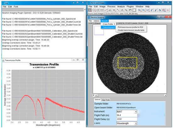
Figure 9.
IMAT ImageJ plugin. The radiography on the right corresponds to a 40 μs time slice at 12 + 20 = 32 ms. On the left, a copper Bragg edge spectrum, averaged for the yellow-box selection, is displayed.
3.4. Correction Procedures
The following operations need to be considered, performed on the stacks of sample and open-beam images (consisting of 2612 individual time slices).
3.4.1. Flat Fielding
The sample data and open-beam stacks are scaled to the same number of incident neutrons, using one of the following: number of neutron pulses; beam monitor integral; an open beam area in the sample image stack; proton current. Both stacks are subjected to artifact cleaning, including a white spot filter. The sample stack is normalized, i.e., by dividing (macro space-time-) pixel by (macro space-time-) pixel, by the open-beam data to yield a stack of transmission images. Note that there is no detector dark noise for the MCP.
3.4.2. MCP Related Corrections
An event overlap correction [57] is performed to take account of the fact that the MCP can register only one neutron per pulse per TOF range (shutter). Hence, a neutron arriving late in the TOF range has a higher probability that a particular pixel is already occupied.
Furthermore, for a quantitative analysis the change of the detection efficiency of the MCP during a measurement may need to be corrected. The efficiency changes under relatively high neutron fluxes due to the ageing effects of current MCPs. Since this efficiency change is position-dependent, it induces a memory image, which can be significantly reduced with correction procedures described in [35].
Misalignment of the quad (2 × 2) Timepix readout chips causes distortions of the real shape of the sample image. The geometry of the gaps can be determined using precision phantoms, and the image distortions can be ameliorated by post-experiment image corrections [58].
3.5. Basic Image Analysis
Figure 10 illustrates a simple image analysis as performed with ImageJ. The test object, and its orientation in the neutron beam, is shown in Figure 10a. Figure 10b represents the ‘white-beam’ transmission image, generated by dividing the respective sums of 2612 slices from the MCP stack for the sample and open-beam data. The white beam radiography shows hardly any contrast between Fe and Cu components. Figure 10c shows a transmission image of averaged time slices 570–580, corresponding to a narrow wavelength band around 3.8 Å, which emphasizes the Cu phase. Similarly, Figure 10d shows a transmission image of averaged time slices 795–805, corresponding to a narrow wavelength band around 4.16 Å, which emphasizes the Fe phase. The selection of wavelengths to highlight one or the other phase is made based on the transmission spectra (Figure 11a) which exhibit, for instance, that the Cu cylinder becomes opaque for a wavelength of 4.16 Å. Figure 10e shows the ratio of two images: the numerator image was obtained by summing wavelength slices between 4.6 and 5.5 Å; the denominator image was obtained by summing wavelength slices between 3.15 and 3.90 Å. The resulting image in Figure 10e enhances the Fe phase. Moreover, it indicated a variation of transmission across the Fe-cylinder by about a factor 2, indicative of texture variations in the outer Fe ring. Similarly, to enhance the Cu phase a ratio-image from regions 4.3–4.4 Å and 4.15–4.17 Å was generated (Figure 10f). The wavelength ranges for generating the ratios for the Fe and Cu enhancements are indicated in Figure 11a. It should be noted that the details about which neutron energies are best to enhance a given material do not need to be known at the time of the data collection. However, care should be taken that there are no (readout) gaps in the relevant ranges of the spectra. An image analysis as shown in Figure 10 emphasizes the advantage of collecting energy-dispersive data, as it leaves a significant amount of flexibility for post-experiment data treatment, e.g., for time binning, event mode analysis and material enhancement.
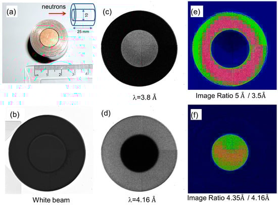
Figure 10.
(a) Photo and sketch of the FeCu test object; (b) normalized white-beam radiography; (c,d) Fe and Cu enhancement by selecting suitable wavelengths; (e,f) Fe and Cu enhancement by producing image ratios from suitable wavelength ranges.
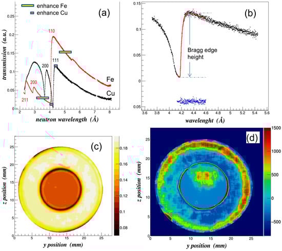
Figure 11.
(a) Bragg edge spectra of Cu and Fe; (b) fit of single Bragg edge; (c) phase fraction map based on Bragg edge heights; (d) relative Bragg edge positions of Fe and Cu.
3.6. Bragg Edge Mapping
The normalized data stack was used to fit Fe and Cu Bragg edges. Spectra from 20 × 20 neighboring pixels were combined to improve the neutron statistics whilst performing a running average with a step size of 55 μm. Inspection of individual spectra of a single pixel and of regions of interest indicated that a binning of 20 × 2055 μm-pixel was adequate, corresponding to a macro-pixel size of 1.1 × 1.1 mm2. The image analysis illustrated in Figure 11 was performed with the BEATRIX [43] neutron transmission analysis tool. Fe(110) and Cu(111) edges were fitted with the analytical function given by Santisteban [17] yielding Bragg edge positions, amplitudes and widths. The wavelength position is used to determine the residual strain
with a reference value λ0 for each hkl-Bragg edge. For strain analysis λ0 corresponds to the Bragg edge position of the unstrained material. With the experiment geometry as indicated in Figure 10a, Equation (3) provides the thickness-averaged axial strain component in microstrain. Here we have not performed d0 measurements for the Fe and Cu parts of the test sample, and hence we do not quantify the axial strain. Rather, values for λ0 = 2 × d0 used were: 4.0538 for Fe(110) and 4.1742 for Cu(111), respectively, calculated from corresponding lattice parameters of 2.8664 Å and 3.6150 Å for Fe and Cu. Figure 11a displays the transmission spectra for the Fe and Cu phases for large regions of interest of 150 × 80 pixels. Figure 11b shows an example of the fit quality for the Cu(111) Bragg edge for a macropixel, superposed on the experimental transmission spectrum (solid black dots), with the blue dots representing the difference, observed minus calculated. Figure 11c exhibits the combined maps of the Bragg edge amplitudes of Fe(110) and Cu(111), thus representing the distribution of the two crystallographic phases. Figure 11c illustrates that by Bragg edge fitting a phase separation can be achieved. Compared to the image manipulation shown in Figure 10, a Bragg edge analysis is capable of providing quantitative results in terms of phase fractions. Figure 11d shows the deviations of the Bragg edge positions from reference values. A prominent ‘tensile’, axisymmetric feature in the outer part of the Fe-ring is observed, as well a non-uniform, asymmetric distribution of Bragg edge shifts for the inner Cu-plug. An interpretation of the maps in terms of axial strains and texture variation (as indicated in Figure 10e,f) will be presented elsewhere, together with neutron diffraction data. It should be noted that composition and strain maps for Fe and Cu were produced in separate analysis steps and combined afterwards for display in Figure 11c,d.
3.7. Tomographic Reconstruction
Where multiple projections are available a 3D volume data of a scalar parameter can be reconstructed using filtered-backprojection or iterative tools. From projections of, for instance, Bragg edge heights (Figure 11c) a 3D volume data can be reconstructed. A study of tomographic reconstruction algorithms of IMAT data is given in [59].
3.8. Discussion
The data collection and analysis work flow for the test object is given as example of an energy-resolving experiment on IMAT. A more thorough analysis and interpretation of the test object data for different strain components, and a comparison with diffraction data will be given elsewhere. Generally, the scan parameters, analysis procedures and software treatment need to be considered and adapted for each case, depending on the experiment’s objectives and experiment conditions (e.g., at non-ambient environments) to achieve, for instance, a certain signal to noise ratio, low contrast feature discrimination or given spatial resolution.
4. Conclusions
The new IMAT instrument is currently being prepared for user operation. Neutron imaging studies on IMAT will be concerned with attenuation-based transmission measurements such as neutron radiography, neutron tomography, and energy-resolved neutron imaging. Other techniques, such as dark field imaging, will be explored in due course. The tomography and energy-resolving options will be used in a diverse range of disciplines including engineering material sciences, hydrogen-related technologies, battery research, earth science and cultural heritage.
Energy-resolved neutron imaging provides a tool for quantitative analysis of phase volume fractions and for mapping texture variations. Currently Bragg edge parameters are mapped with a spatial resolution of a few hundred microns. Analysis of the wavelength dependencies of Bragg edge parameters allows studying microstructure feature such as particle size and microstrain. TOF image analysis is in its infancy and advanced analysis algorithms and tools for reduction and analysis of energy-dispersive imaging data are developed for particular science projects. Further gains in terms of collection times and spatial resolution are to be expected with structure-constrained multi-edge and Rietveld-type analyses approaches. For scalar parameters such as phase fractions the extension from 2D to 3D imaging is straightforward as has been demonstrated by Woracek et al. [24]. Strain gradients can be mapped, while a full strain analysis via Bragg edge transmission is hampered due to the ill-posed problem for strain tomography [22]. The transmission analysis of structure-related properties including residual strains and texture will, however, benefit from the additional information from the diffraction detectors which are in the process of being installed on IMAT.
Acknowledgments
We acknowledge support throughout the IMAT project via the collaboration for scientific research at the ISIS spallation neutron source under CNR-STFC Agreement 2014–2020 (No. 3420 2014-2020). AST and JBM would like to acknowledge the collaboration between UC Berkeley and Nova Scientific, partially funded by the US Department of Energy under STTR grant Nos. DE-FG02-07ER86322, DE-FG02-08ER86353 and DE-SC0009657, and the Medipix collaboration for development of the MCP detector and Timepix readout, respectively. KW acknowledges support by the JSPS Programme, Japan, for Advancing Strategic International Networks to Accelerate the Circulation of Talented Researchers.
Author Contributions
The work performed in the IMAT instrumentation and commissioning project was performed in collaboration between all authors. W.K., T.M., D.E.P., G.B., R.R. collected and analysed the data. T.M. and A.S.T. developed the TOF data analysis codes. F.A.A., G.D.H., C.M., D.P.K. developed the instrument control user interfaces; J.K., S.K., T.-L.L., R.Z., A.R., G.V., D.M. tested the interfaces and software tools; D.E.P., J.W.L.L., A.S.T., J.B.M. developed the TOF cameras; F.A., R.P., S.T., G.S., C.V. G.G. developed the optical camera box. G.V., D.M.; R.G.A., V.F. developed correction tools and tested reconstruction algorithms; K.W. developed MCP correction procedures; F.G. helped developing the pinhole selector; D.N., ND. developed the MANTID imaging tools; W.H., J.N. produced the engineering design drawings. All authors discussed the results and commented on the manuscript at all stages.
Conflicts of Interest
The authors declare no conflict of interest.
References
- Kockelmann, W.; Frei, G.; Lehmann, E.H.; Vontobel, P.; Santisteban, J.R. Energy-selective neutron transmission imaging at a pulsed source. Nucl. Instrum. Meth. 2007, A57, 421–434. [Google Scholar] [CrossRef]
- Shinohara, T.; Kai, T.; Oikawa, K.; Segawa, M.; Harada, M.; Nakatani, T.; Ooi, M.; Aizawa, K.; Sato, H.; Kamiyama, T.; et al. Final design of the energy-resolved neutron imaging system RADEN at J-PARC. J. Phys. Conf. Ser. 2016, 746, 012007. [Google Scholar] [CrossRef]
- Strobl, M. Future prospects of imaging at spallation neutron sources. Nucl. Instrum. Meth. 2009, A604, 646–652. [Google Scholar] [CrossRef]
- Strobl, M.; Kardjilov, N.; Hilger, A.; Penumadu, D.; Manke, I. Advanced neutron imaging methods with a potential to benefit from pulsed sources. Nucl. Instrum. Meth. 2011, A651, 57–61. [Google Scholar] [CrossRef]
- Kabra, S.; Kelleher, J.; Kockelmann, W.; Gutmann, M.; Tremsin, A.S. Energy-dispersive neutron imaging and diffraction of magnetically driven twins in a Ni2MnGa single crystal magnetic shape memory alloy. J. Phys. Conf. Ser. 2016, 746, 012056. [Google Scholar] [CrossRef]
- Tremsin, A.S.; Yau, T.Y.; Kockelmann, W. Non-destructive examination of loads in regular and self-locking Spiralock® threads through energy-resolved neutron imaging. Strain 2016, 52, 548–558. [Google Scholar] [CrossRef]
- Sato, H.; Shiota, Y.; Morooka, S.; Todaka, Y.; Adachi, N.; Sadamatsu, S.; Oikawa, K.; Harada, M.; Zang, S.; Su, Y.; et al. Inverse pole figure mapping of bulk crystalline grains in a polycrystalline steel plate by pulsed neutron Bragg-dip transmission imaging. J. Appl. Cryst. 2017, 50, 1601–1610. [Google Scholar] [CrossRef]
- Makowska, M.G.; Strobl, M.; Lauridsen, E.M.; Kabra, S.; Kockelmann, W.; Tremsin, A.; Frandsen, H.L.; Theil Kuhn, L. In situ time-of-flight neutron imaging of NiO–YSZ anode support reduction under influence of stress. J. Appl. Cryst. 2016, 49, 1674–1681. [Google Scholar] [CrossRef]
- Festa, G.; Perelli Cippo, E.; Di Martino, D.; Cattaneo, R.; Senesi, R.; Andreani, C.; Schooneveld, E.; Kockelmann, W.; Rhodes, N.; Scherillo, A.; et al. Neutron resonance transmission imaging for 3D elemental mapping at the ISIS spallation neutron source. J. Anal. At. Spectrom. 2015, 30, 745–750. [Google Scholar] [CrossRef]
- Tremsin, A.S.; Vogel, S.C.; Mocko, M.; Bourke, M.A.M.; Yuan, V.; Nelson, R.O.; Brown, D.W.; Feller, W.B. Non-destructive studies of fuel rodlets by neutron resonance absorption radiography and thermal neutron radiography. J. Nucl. Mater. 2013, 440, 633–646. [Google Scholar] [CrossRef]
- Kai, T.; Maekawa, F.; Oshita, H.; Sato, H.; Shinohara, T.; Ooi, M.; Harada, M.; Uno, S.; Otomo, T.; Kamiyama, T.; et al. Visibility estimation for neutron resonance absorption radiography using a pulsed neutron source. Phys. Procedia 2013, 43, 111–120. [Google Scholar] [CrossRef]
- Tremsin, A.S.; Kockelmann, W.; Pooley, D.E.; Feller, W.B. Spatially resolved remote measurement of temperature by neutron resonance absorption. Nucl. Instrum. Meth. A 2015, 803, 15–23. [Google Scholar] [CrossRef]
- Shinohara, T.; Hiroi, K.; Su, Y.; Kai, T.; Nakatani, T.; Oikawa, K.; Segawa, M.; Hayashida, H.; Parker, J.D.; Matsumoto, Y.; et al. Polarization analysis for magnetic field imaging at RADEN in J-PARC/MLF. J. Phys. Conf. Ser. 2017, 862, 012025. [Google Scholar] [CrossRef]
- Cereser, A.; Strobl, M.; Hall, S.A.; Steuwer, A.; Kiyanagi, Y.; Tremsin, A.S.; Knudsen, E.B.; Shinohara, T.; Willendrup, P.K.; Bastos da Silva Fanta, A.; et al. Time-of-Flight Three Dimensional Neutron Diffraction in Transmission Mode for Mapping Crystal Grain Structures. Sci. Rep. 2017, 7, 9561. [Google Scholar] [CrossRef] [PubMed]
- Strobl, M.; Betz, B.; Harti, R.P.; Hilger, A.; Kardjilov, N.; Manke, I.; Gruenzweig, C. Wavelength-dispersive dark-field contrast: Micrometre structure resolution in neutron imaging with gratings. J. Appl. Cryst. 2016, 49, 569–573. [Google Scholar] [CrossRef]
- Vogel, S. A Rietveld-Approach for the Analysis of Neutron Time-of-Flight Transmission Data. Ph.D. Thesis, Christian Albrechts Universität, Kiel, Germany, 2000. [Google Scholar]
- Santisteban, J.R.; Edwards, L.; Steuwer, A.; Withers, P.J. Time-of-flight neutron transmission diffraction. J. Appl. Crystallogr. 2001, 34, 289–297. [Google Scholar] [CrossRef]
- Santisteban, J.R.; Vicente-Alvarez, M.A.; Vizcaino, P.; Banchik, A.D.; Vogel, S.C.; Tremsin, A.S.; Vallerga, J.V.; McPhate, J.B.; Lehmann, E.; Kockelmann, W. Texture imaging of zirconium based components by total neutron cross-section experiments. J. Nucl. Mater. 2012, 425, 218–227. [Google Scholar] [CrossRef]
- Tremsin, A.S.; Ganguly, S.; Meco, S.M.; Pardal, G.R.; Shinohara, T.; Feller, W.B. Investigation of dissimilar metal welds by energy resolved neutron imaging. J. Appl. Cryst. 2016, 49, 1130–1140. [Google Scholar] [CrossRef] [PubMed]
- Vitucci, G.; Minniti, T.; Di Martino, D.; Musa, M.; Gori, L.; Micieli, D.; Kockelmann, W.; Watanabe, K.; Tremsin, A.S.; Gorini, G. Energy-resolved neutron tomography of an unconventional cultured pearl at a pulsed spallation source using a microchannel plate camera. Microchem. J. 2018, 137, 473–479. [Google Scholar] [CrossRef]
- Hendriks, J.N.; Gregg, A.W.T.; Wensrich, C.M.; Tremsin, A.S.; Shinohara, T.; Meylan, M.; Kisi, E.H.; Luzin, V.; Kirsten, O. Bragg-edge elastic strain tomography for in situ systems from energy-resolved neutron transmission imaging. Phys. Rev. Mater. 2017, 1, 053802. [Google Scholar] [CrossRef]
- Lionheart, W.R.B.; Withers, P.J. Diffraction tomography of strain. Inverse Probl. 2015, 31, 045005. [Google Scholar] [CrossRef]
- Kardjilov, N.; Manke, I.; Hilger, A.; Williams, S.; Strobl, M.; Woracek, R.; Boin, M.; Lehmann, E.; Penumadu, D.; Banhart, J. Neutron Bragg edge mapping of weld seams. Int. J. Mater. Res. 2012, 103, 151–154. [Google Scholar] [CrossRef]
- Woracek, R.; Penumadu, D.; Kardjilov, N.; Hilger, A.; Boin, M.; Banhart, J.; Manke, I. 3D Mapping of Crystallographic Phase Distribution using Energy-Selective Neutron Tomography. Adv. Mater. 2014, 26, 4069–4073. [Google Scholar] [CrossRef] [PubMed]
- Minniti, T.; Kockelmann, W.; Burca, G.; Kelleher, J.F.; Kabra, S.; Zhang, S.Y.; Pooley, D.E.; Schooneveld, E.M.; Mutamba, Q.; Sykora, J.; et al. Materials analysis opportunities on the new neutron imaging facility IMAT@ISIS. J. Instrum. 2016, 11, C03014. [Google Scholar] [CrossRef]
- Kockelmann, W.; Burca, G.; Kelleher, J.F.; Kabra, S.; Zhang, S.Y.; Rhodes, N.J.; Schooneveld, E.M.; Sykora, J.; Pooley, D.E.; Nightingale, J.B.; et al. Status of the neutron imaging and diffraction instrument IMAT. Phys. Procedia 2015, 69, 71–78. [Google Scholar] [CrossRef]
- Strobl, M. The Scope of the Imaging Instrument Project ODIN at ESS. Phys. Procedia 2015, 69, 18–26. [Google Scholar] [CrossRef]
- Bilheux, H.; Herwig, K.; Keener, S.; Davis, L. Overview of the conceptual design of the future VENUS neutron imaging beam line at the Spallation Neutron Source. Phys. Procedia 2015, 69, 55–59. [Google Scholar] [CrossRef]
- Minniti, T.; Watanabe, K.; Burca, G.; Pooley, D.E.; Kockelmann, W. Characterization of the new neutron imaging and materials science facility IMAT. Nucl. Instrum. Meth. A 2018, A888, 184–195. [Google Scholar] [CrossRef]
- Vallance, C.; Brouard, M.; Lauer, A.; Slater, C.S.; Halford, E.; Winter, B.; King, S.J.; Lee, J.W.L.; Pooley, D.E.; Sedgwick, I.; et al. Fast sensor for time-of-flight imaging applications. Phys. Chem. Chem. Phys. 2014, 16, 383–395. [Google Scholar] [CrossRef] [PubMed]
- Pooley, D.E.; Lee, J.W.L.; Brouard, M.; John, J.J.; Kockelmann, W.; Rhodes, N.J.; Schooneveld, E.M.; Sedgwick, I.; Turchetta, R.; Vallance, C. Development of the GP2 Detector: Modification of the PImMS CMOS Sensor for Energy-Resolved Neutron Radiography. IEEE Trans. Nucl. Sci. 2017, 64, 2970–2981. [Google Scholar] [CrossRef]
- Tremsin, A.S.; Vallerga, J.V.; McPhate, J.B.; Siegmund, O.H.W.; Raffanti, R. High Resolution Photon Counting with MCP-Timepix Quad Parallel Readout Operating at > 1 KHz Frame Rates. IEEE Trans. Nucl. Sci. 2013, 60, 578–585. [Google Scholar] [CrossRef]
- Parker, J.D.; Harada, M.; Hattori, K.; Iwaki, S.; Kabuki, S.; Kishimoto, Y.; Kubo, H.; Kurosawa, S.; Matsuoka, Y.; Miuchi, K.; et al. Spatial resolution of a µPIC−based neutron imaging detector. Nucl. Instrum. Meth. 2013, A726, 155–161. [Google Scholar] [CrossRef]
- Finocchiaro, V.; Aliotta, F.; Tresoldi, D.; Ponterio, R.C.; Vasi, C.S.; Salvato, G. The autofocusing system of the IMAT neutron camera. Rev. Sci. Instrum. 2013, 84, 093701. [Google Scholar] [CrossRef] [PubMed]
- Watanabe, K.; Minniti, T.; Kockelmann, W.; Dalgliesh, R.; Burca, G.; Tremsin, A.S. Characterization of a neutron sensitive MCP/Timepix detector for quantitative image analysis at a pulsed neutron source. Nucl. Instrum. Meth. 2017, A861, 55–63. [Google Scholar] [CrossRef]
- Akeroyd, F.A.; Baker, K.V.L.; Clarke, M.J.; Holt, J.R.; Howells, G.D.; Keymer, D.P.; Löhnert, T.; Moreton-Smith, C.M.; Oram, D.E.; Potter, A.; et al. IBEX—An EPICS based control system for the ISIS pulsed neutron and muon source. In Proceedings of the International Conference on Advanced Neutron Sources (ICANS-XII), Oxford, UK, 27–31 March 2018. in press. [Google Scholar]
- EPICS: Experimental Physics and Industrial Control System URL. Available online: http://www.aps.anl.gov/epics/ (accessed on 2 January 2018).
- EPICS OPI. Available online: http://controlsystemstudio.org/ (accessed on 2 January 2018).
- Uno, S.; Uchida, T.; Sekimoto, M.; Murakami, T.; Miyama, K.; Shoji, M.; Nakano, E.; Koike, T.; Morita, K.; Sato, H.; et al. Two-dimensional Neutron Detector with GEM and its Applications. Phys. Procedia 2012, 26, 142–152. [Google Scholar] [CrossRef]
- Turecek, D.; Holy, T.; Jakubek, J.; Pospisil, S.; Vykydal, Z. Pixelman: A multi-platform data acquisition and processing software package for Medipix2, Timepix and Medipix3 detectors. J. Instrum. 2011, 6, C01046. [Google Scholar] [CrossRef]
- Koennecke, M.; Akeroyd, F.A.; Bernstein, H.J.; Brewster, A.S.; Campbell, S.I.; Clausen, B.; Cottrell, S.; Hoffmann, J.U.; Jemian, P.R.; Maennicke, D.; et al. The NeXus data format. J. Appl. Cryst. 2015, 48, 301–305. [Google Scholar] [CrossRef] [PubMed]
- NeXus Application De_nition NXtomo URL. Available online: http://download.nexusformat.org/sphinx/classes/applications/NXtomo.html (accessed on 2 January 2018).
- Minniti, T. BEATRIX TOF Analysis Code. Private communication 2017.
- Tremsin, A.S. TOF Analysis Code. Private communication 2017.
- Sato, H.; Watanabe, K.; Kiyokawa, K.; Kiyanagi, R.; Hara, K.Y.; Kamiyama, T.; Furusaka, M.; Shinohara, T.; Kiyanagi, Y. Further improvement of the RITS code for pulsed neutron Bragg-edge transmission imaging. Phys. Procedia 2017, 88, 322–330. [Google Scholar] [CrossRef]
- Available online: https://octopusimaging.eu/ (accessed on 2 January 2018).
- Guersoy, D.; Carlo, F.D.; Xiao, X.; Jacobsen, C. Tomopy: A framework for the analysis of synchrotron tomographic data. J. Synchrotron Radiat. 2014, 21, 1188–1193. [Google Scholar] [CrossRef] [PubMed]
- AstraToolbox URL. Available online: https://github.com/astra-toolbox/astra-toolbox/ (accessed on 2 January 2018).
- Available online: https://www.volumegraphics.com/en/products/vgstudio-max.html (accessed on 2 January 2018).
- Available online: https://www.fei.com/software/amira-avizo/ (accessed on 2 January 2018).
- Mantid 2015 Manipulation and Analysis Toolkit for Instrument Data. Mantid Project. Available online: http://dx.doi.org/10.5286/SOFTWARE/MANTID3.5 (accessed on 2 January 2018).
- Savu: Tomography Reconstructon Pipeline. Available online: https://github.com/DiamondLightSource/Savu (accessed on 2 January 2018).
- Atwood, R.C.; Bodey, A.J.; Price, S.W.T.; Basham, M.; Drakopoulos, M. A high-throughput system for high-quality tomographic reconstruction of large datasets at Diamond Light Source. Philos. Trans. R. Soc. A 2015, 373, 20140398. [Google Scholar] [CrossRef] [PubMed]
- Steuwer, A.; Withers, P.J.; Santisteban, J.R.; Edwards, L. Using pulsed neutron transmission for crystalline phase imaging and analysis. J. Appl. Phys. 2005, 97, 074903. [Google Scholar] [CrossRef]
- Boin, M. NXS: A program library for neutron cross section calculations. J. Appl. Crystallogr. 2012, 45, 603–607. [Google Scholar] [CrossRef]
- Burca, G.; Kelleher, J.; Peacock, A.; Hayes, M.; Deliry, P. An integrated tool for Bragg Edge analysis at ISIS. In Proceedings of the NEUWAVE-8 Workshop, Abingdon UK, 12–15 June 2016. [Google Scholar]
- Tremsin, A.S.; Vallerga, J.V.; McPhate, J.B.; Siegmund, O.H.W. Optimization of Timepix count rate capabilities for the applications with a periodic input signal. J. Instrum. 2014, 9, C05026. [Google Scholar] [CrossRef]
- Vitucci, G.; Minniti, T.; Tremsin, A.S.; Kockelmann, W.; Gorini, G. Investigation of image distortion due to MCP electronic readout misalignment and correction via customized GUI application. J. Instrum. 2018. under review. [Google Scholar]
- Micieli, D.; Minniti, T.; Formoso, V.; Kockelmann, W.; Gorini, G. A comparative study of reconstruction methods applied to neutron tomography. J. Instrum. 2017. under review. [Google Scholar]


© 2018 by the authors. Licensee MDPI, Basel, Switzerland. This article is an open access article distributed under the terms and conditions of the Creative Commons Attribution (CC BY) license (http://creativecommons.org/licenses/by/4.0/).