Article

Efficient Lossless Compression of Multitemporal Hyperspectral Image Data

1
Bank of America Corporation, New York, NY 10020, USA
2
Department of Electrical and Computer Engineering, University of Alabama in Huntsville, Huntsville, AL 35899, USA
*
Author to whom correspondence should be addressed.
Note: This paper is continuation of the first author’s PhD work, which is not associated with his current affiliation.
J. Imaging 2018, 4(12), 142; https://doi.org/10.3390/jimaging4120142
Submission received: 14 November 2018 / Accepted: 27 November 2018 / Published: 2 December 2018
(This article belongs to the Special Issue The Future of Hyperspectral Imaging)

Abstract

:
Hyperspectral imaging (HSI) technology has been used for various remote sensing applications due to its excellent capability of monitoring regions-of-interest over a period of time. However, the large data volume of four-dimensional multitemporal hyperspectral imagery demands massive data compression techniques. While conventional 3D hyperspectral data compression methods exploit only spatial and spectral correlations, we propose a simple yet effective predictive lossless compression algorithm that can achieve significant gains on compression efficiency, by also taking into account temporal correlations inherent in the multitemporal data. We present an information theoretic analysis to estimate potential compression performance gain with varying configurations of context vectors. Extensive simulation results demonstrate the effectiveness of the proposed algorithm. We also provide in-depth discussions on how to construct the context vectors in the prediction model for both multitemporal HSI and conventional 3D HSI data.

1. Introduction

Hyperspectral imaging (HSI) technologies have been widely used in many applications of remote sensing (RS) owing to the high spatial and spectral resolutions of hyperspectral images [1]. In some applications (e.g., hyperspectral imaging change detection [2,3,4,5]), we need to collect a sequence of hyperspectral images over the same spatial area at different times. The set of hyperspectral images collected over one location at varying time points is called multitemporal hyperspectral images [6,7]. From these multitemporal images, changes of observed locations over time can be detected and analyzed. 
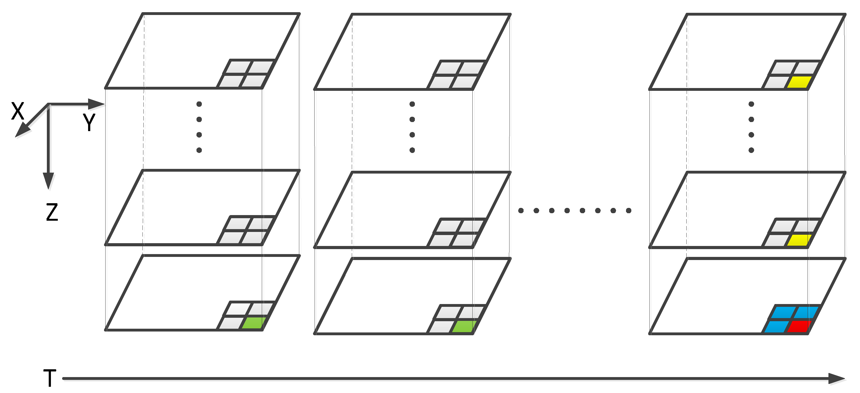
Figure 1 illustrates a typical multitemporal hyperspectral image dataset. Each stack represents one 3D HSI. A sequence of 3D HSI stacks are captured by the HSI sensor over time.
Hyperspectral datasets tend to be of very large sizes. In the case of 4D multitemporal HSI datasets, the accumulated data volume increases very rapidly (to the Gigabyte or even Terabyte level), thereby making data acquisition, storage and transmission very challenging, especially when network bandwidth is severely constrained. As the number of hyperspectral images grows, it is clear that data compression techniques play a crucial role in the development of hyperspectral imaging techniques [8,9]. Lossy compression can significantly improves the compression efficiency, albeit at the cost of selective information loss. However, the fact that human visual systems are not sensitive to certain types and levels of distortions caused by information loss makes lossy compression useful. While lossy compression methods typically provide much larger data reduction than lossless methods, they might not be suitable for many accuracy-demanding hyperspectral imaging applications, where the images are intended to be analyzed automatically by computers. Since lossless compression methods can strictly guarantee no loss in the reconstructed data, lossless compression would be more desirable in these applications.
Many efforts have been made to develop efficient lossless compression algorithms for 3D HSI data. LOCO-I [10] and 2D-CALIC [11] utilize spatial redundancy to reduce the entropy of prediction residuals. To take advantage of strong spectral correlations in HSI data, 3D compression methods have been proposed, which includes 3D-CALIC [12], M-CALIC [13], LUT [14] and its variants, SLSQ [15] and CCAP [16]. Also, some transform-based methods, such as SPIHT [17], SPECK [18], etc., can be easily extended to lossless compression even though they were designed for lossy compression.
Recently, clustering techniques have been introduced into 3D HSI data lossless compression and produced state-of-the-art performance over publicly available datasets. In [19], B. Aiazzi et al. proposed a predictive method leveraging crisp or fuzzy clustering to produce state-of-the-art results. Later, authors in both [20,21] again utilized the K-means clustering algorithm to improve the compression efficiency. Although these methods can yield higher compression, their computational costs are significantly higher than regular linear predictive methods. Plus, it is very difficult to parallel the process to leverage hardware acceleration if clustering technique is required as a preprocessing step in those approaches. In addition to the goal of reducing the entropy of either prediction residuals or transform coefficients, low computational complexity is another influential factor because many sensing platforms have very limited computing resources. Therefore, a low-complexity method called the “Fast Lossless” (FL) method, proposed by the NASA Jet Propulsion Lab (JPL) in [22], was selected as the core predictor in the Consultative Committee for Space Data Systems (CCSDS) new standard for multispectral and hyperspectral data compression [23], to provide efficient compression on 3D HSI data. This low-complexity merit also enables efficient multitemporal HSI data compression.
Multitemporal HSI data has an additional temporal dimension compared to 3D HSI data. Therefore, we can take advantage of temporal correlations to improve the overall compression efficiency of 4D HSI data. Nonetheless, there is very sparse work on lossless compression of multitemporal HSI data in the literature. Mamun et al. proposed a 4D lossless compression algorithm in [24], albeit lacking details on the prediction algorithms. In [25], a combination of Karhunen-Loève Transform (KLT), Discrete Wavelet Transform (DWT), and JPEG 2000 was applied to reduce the spectral and temporal redundancy of 4D remote sensing image data. However, the method can only achieve lossy compression. Additionally, Zhu et al. proposed another lossy compression approach for multitemporal HSI data in [7], based on a combination of linear prediction and a spectral concatenation of images. For the first time, we addressed lossless compression of multitemporal HSI data in [6], by introducing a correntropy based Least Mean Square filter for the Fast Lossless (FL) predictor. While the benefit of exploiting temporal correlations in compression has been demonstrated by some papers such as [26,27], in this work, we conduct an in-depth information-theoretic analysis on the amount of compression achievable on multitemporal HSI data, by taking into account both the spectral and temporal correlations. On the other hand, this additional temporal decorrelation definitely poses a greater challenge to data processing speed especially for those powerful but computationally expensive algorithms, e.g., [19,20,21]. Therefore, we propose a low-complexity linear prediction algorithm, which extends the well-known FL method into a 4D version to achieve higher data compression, by better adapting to the underlying statistics of multitemporal HSI data. Note that most existing 3D HSI compression methods can be extended into 4D versions with proper modifications. However, this is beyond the scope of this paper.
The remainder of this paper is organized as follows. First, in Section 2, we give an overview of the multitemporal HSI datasets used in the study, which include three publicly available datasets, as well as two multitemporal HSI datasets we generated by using hyperspectral cameras. In Section 3, we present the information-theoretic analysis, followed by the introduction of a new algorithm for multitemporal HSI data lossless compression in Section 4. Finally, we present simulation results in Section 5 and make some concluding remarks in Section 6.

2. Datasets

Since there is little prior work on multi-temporal hyperspectral image compression, publicly available multi-temporal HSI datasets are very rare. Currently, the time-lapse hyperspectral radiance images of natural scenes [28] are the only available datasets to our best knowledge. Therefore, we created another two datasets capturing two scenes of Alabama A&M University campus using the portable Surface Optics Corporation (SOC) 700 hyperspectral camera [29] to enrich the relevant resources and facilitate further research. Hence, we introduce both data sources especially our datasets in detail before the actual analysis and algorithm development.

2.1. Time-Lapse Hyperspectral Imagery

Time-lapse hyperspectral imaging technology has been used for various remote sensing applications due to its excellent capability of monitoring regions-of-interest over a period of time. Time-lapse hyperspectral imagery is a sequence of 3D HSIs captured over the same scene but at different time stamps (often at a fixed time interval). Therefore, time-lapse hyperspectral imagery can be considered as a 4D dataset, whose size increases significantly with the total number of time stamps.
In [28], the authors made public several sequences of hyperspectral radiance images of scenes undergoing natural illumination changes. In each scene, hyperspectral images were acquired at about one-hour intervals. We randomly selected three 4D time-lapse HSI datasets, Levada, Gualtar and Nogueiro. Basic information of these three datasets are listed in the Table 1. Detailed information of these datasets can be found in [30]. Each single HSI has the same spatial size, 1024 × 1344 , with 33 spectral bands. Both Gualtar and Nogueiro have nine time stamps while Levada has seven. Note that the original data for these datasets was linearly mapped into [ 0 , 1 ] and stored using “double” floating point format (64 bits) [28]. In order to evaluate the prediction-based lossless compression performance of algorithms, we pre-process the datasets by re-mapping the data samples back to their original precision of 12 bits. The resulting sizes of the datasets range from 454.78 MB (for seven frames) to 584.71 MB (for nine frames).
Figure 2 shows the Levada, Noguerio and Gualtar sequences from top to bottom. Detailed information about the Levada sequence can be found in [28]. Note that only 2D color-rendered RGB (Red, Green and Blue) images are shown in Figure 2 instead of the actual HSI data for display purpose. Since time-lapse HSIs are captured over the same scene at different time instants with gradually changing natural illumination, we can see that images at different time instants are very similar in Figure 2. These temporal correlations can be exploited to improve the overall compression efficiency.

2.2. AAMU Datasets

Due to very few 4D HSI datasets available in the public domain, we created some new datasets to increase the data diversity of our study. To this end, we used a SOC 700 hyperspectral camera (manufactured by Surface Optics Corporstion, CA, USA) and produced 4D datasets for two scenes on the campus of Alabama A&M University (AAMU). The SOC 700 camera can record and process hyperspectral imagery at a rate of 15 megabytes of data every second (120-band elements per second at 12-bit resolution, 640 pixels per row, 100 rows per second). The imaging system’s spectral response covers the visible and near-infrared spectral range (from 0.43 to 0.9 microns), and can be used in normal to low lighting conditions with variable exposure times and display gains. More detailed about the SOC 700 system can be found at [29].
We placed the camera at two distinct locations of the AAMU campus and generated two datasets, which we call Scene-1 and Scene-2. 3D HSI cubes in Scene-1 and Scene-2 are of the same size: 640 × 640 × 120 with 21 and 16 time frames, respectively. The overall dataset sizes of Scene-1 and Scene-2 are roughly 1.70 GB and 850 MB, respectively. Compared to three time-lapse datasets discussed earlier, these two AAMU datasets are much larger, making themselves more suitable for evaluating compression efficiencies. In contrast to the time-lapse datasets, the images of the AAMU datasets were acquired at time-varying rates of approximately one per five minutes or one per minute, thereby introducing time-varying temporal correlations through the entire dataset. This special feature will allow us to investigate the relationship between prediction accuracy and correlations at different levels.
Figure 3 shows the 2D color-rendered RGB images for a few time instants for the AAMU multitemporal HSI datasets. While changing illumination conditions over time can be observed in both datasets, temporal similarity in both pixel intensity and image structure is also obvious, similar to the three time-lapse datasets shown in Figure 2. In order to quantify the potential gain on compression achievable by exploiting the temporal correlations in 4D HSI datasets, we conducted an information-theoretic analysis as detailed in the next section.

3. Problem Analysis

While the actual amount of compression achieved depends on the choice of specific compression algorithms [31], information theoretic analysis can provide us an upper bound on the amount of compression achievable. Here we focus on analyzing how temporal correlation can help improve the compression of 4D hyperspectral image datasets, as opposed to the baseline 3D-compression case where only spatial and spectral correlations are considered.
Let X j t be a 4D hyperspectral image at the tth time instant and jth spectral band where X represents a two-dimensional image with K distinct pixel values v i ( i { 1 , , K } ) within each band. Then the entropy of this source can be obtained based on the probabilities p ( v i ) of these values by
H ( X j t ) = i = 1 K p ( v i ) · log 2 p ( v i ) .
If we assume that there are no dependencies between pixels of X j t , at least H ( X j t ) bits must be spent on average for each pixel of this image. However, for typical 4D hyperspectral images, this assumption does not hold given the existence of spatial, spectral and temporal correlations. The value of a particular pixel might be similar to some other pixels from its spatial, spectral or temporal neighborhoods (contexts). Considering these correlations can lead to reduced information (fewer bits to code each pixel on average) than the entropy H ( X j t ) . The conditional entropy of the image captures the correlations as follows:
H ( X j t | C j t ) = i = 1 K p ( v i | C j t ) · log 2 p ( v i | C j t ) .
where C j t denoted as context, which represents a group of correlated pixels. In general, conditioning reduces entropy, H ( X j t | C j t ) H ( X j t ) .
The choice of context largely determines how much compression we can achieve by using prediction-based lossless compression schemes. One should include highly-correlated pixels into the context. Spectral and temporal correlations are typically much stronger than spatial correlations in multitemporal hyperspectral images. For example, ref. [20] claims that explicit spatial de-correlation is not always necessary to achieve good compression [31]. Ref. [31] shows that a linear prediction scheme was adequate for spectral and/or temporal prediction because of high degree of correlations, in contrast to non-linearity nature of spatial de-correlation. Therefore, we construct the context vector C j t using only pixels from previous bands at the same spatial location, as well as pixels from the same spectral band at the same location but at previous time points. Specifically, we denote pixels from previous N b bands at the same spatial location as X j m t , m { 1 , 2 , , N b } (yellow pixels in Figure 1), and pixels from the same spectral band at the same location but from previous N t temporal positions X j t n , n { 1 , 2 , , N t } (green pixels in Figure 1), respectively. Then, the conditional entropy in Equation (2) becomes   
H ( X j t | X j m t , X j t n ) = i = 1 K p ( v i | X j m t , X j t n ) · log 2 p ( v i | X j m t , X j t n ) .
By using the relation between joint entropy and conditional entropy, we can further rewrite Equation (3) as
H ( X j t | X j m t , X j t n ) = H ( X j t , X j m t , X j t n ) H ( X j m t , X j t n ) ,
which enables a simple algorithm for estimation of the conditional entropies. It suffices to estimate the above two joint entropies by counting the occurrence frequency of each ( N t + N b + 1 ) -tuple in the set ( X j t , X j m t , X j t n ) , and ( N t + N b ) -tuple in the set ( X j m t , X j t n ) , respectively. However, as pointed out in  [31], the entropy estimates become very inaccurate when two or more previous bands are used for prediction in practice. The reason is that, as the entropy is conditioned upon multiple bands, the set ( X j t , X j m t , X j t n ) takes on values from the alphabet χ ( N t + N b + 1 ) , whose size can become extremely large, e.g., ( 2 12 ) N t + N b + 1 for our datasets. As a consequence, a band might not contain enough pixels to provide statistically meaningful estimates of the probabilities. Similar to the “data source transform” trick proposed in [31], we consider each bit-plane of X j t as one separate binary source. Although binary sources greatly reduce the alphabet size, which makes it possible to obtain accurate entropy estimates, results obtained for the binary source are not very representative of the actual bit rates obtained by a practical coder since statistical dependencies between those bit-planes cannot be neglected. However, using bit-plane sources would be useful for our study since our main goal is to evaluate the relative instead of the absolute performance gain achievable by using different contexts based on various combinations of spectral and temporal bands. Therefore, we will compute the conditional entropy in Equation 3, for all the bit-planes separately, and then take their average to be the overall performance gain for a specific prediction context. In this sense, we extend the algorithm in [31] by incorporating previous temporal bands into the context vector, which allows us to estimate also the temporal correlations.
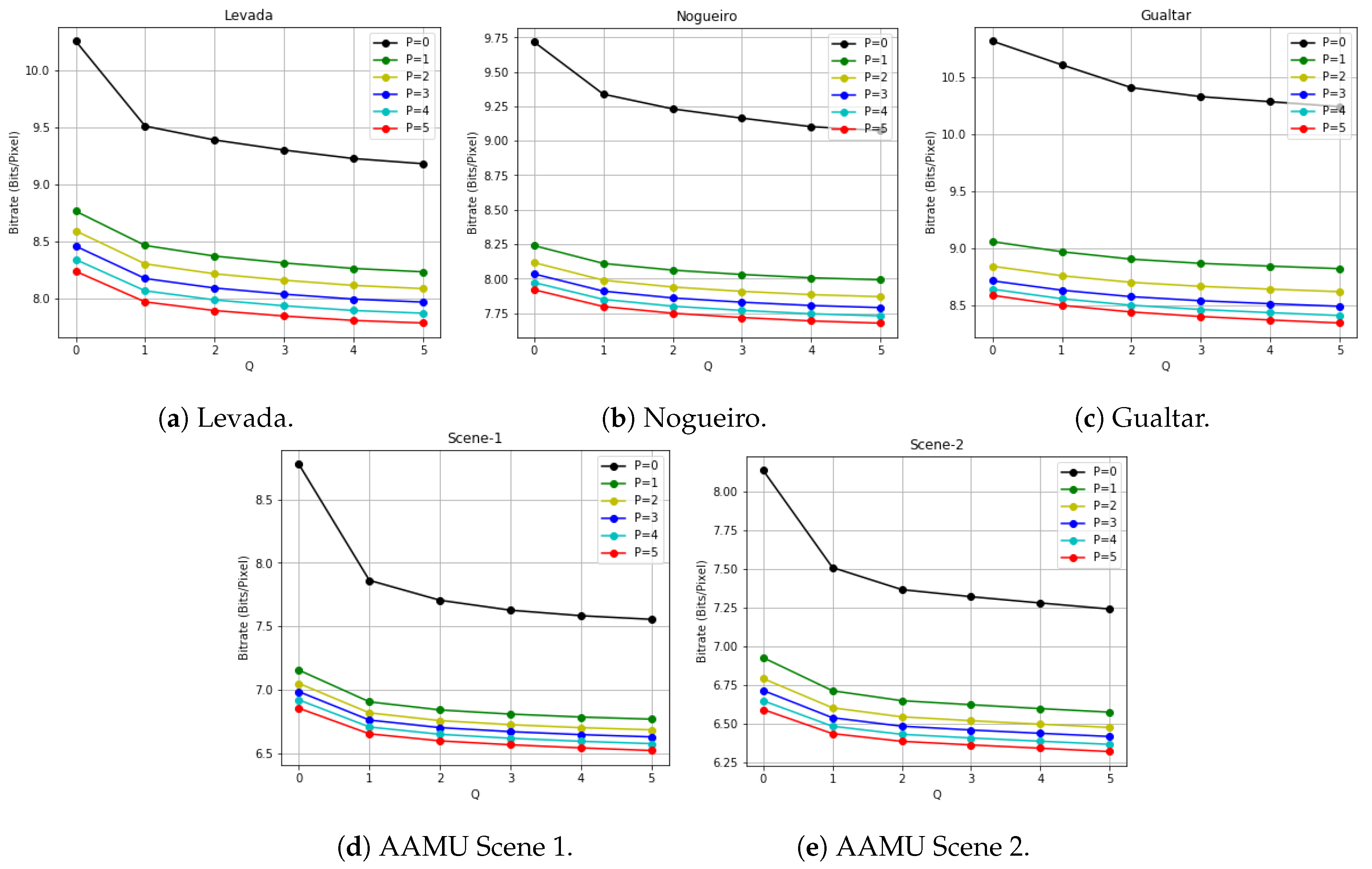
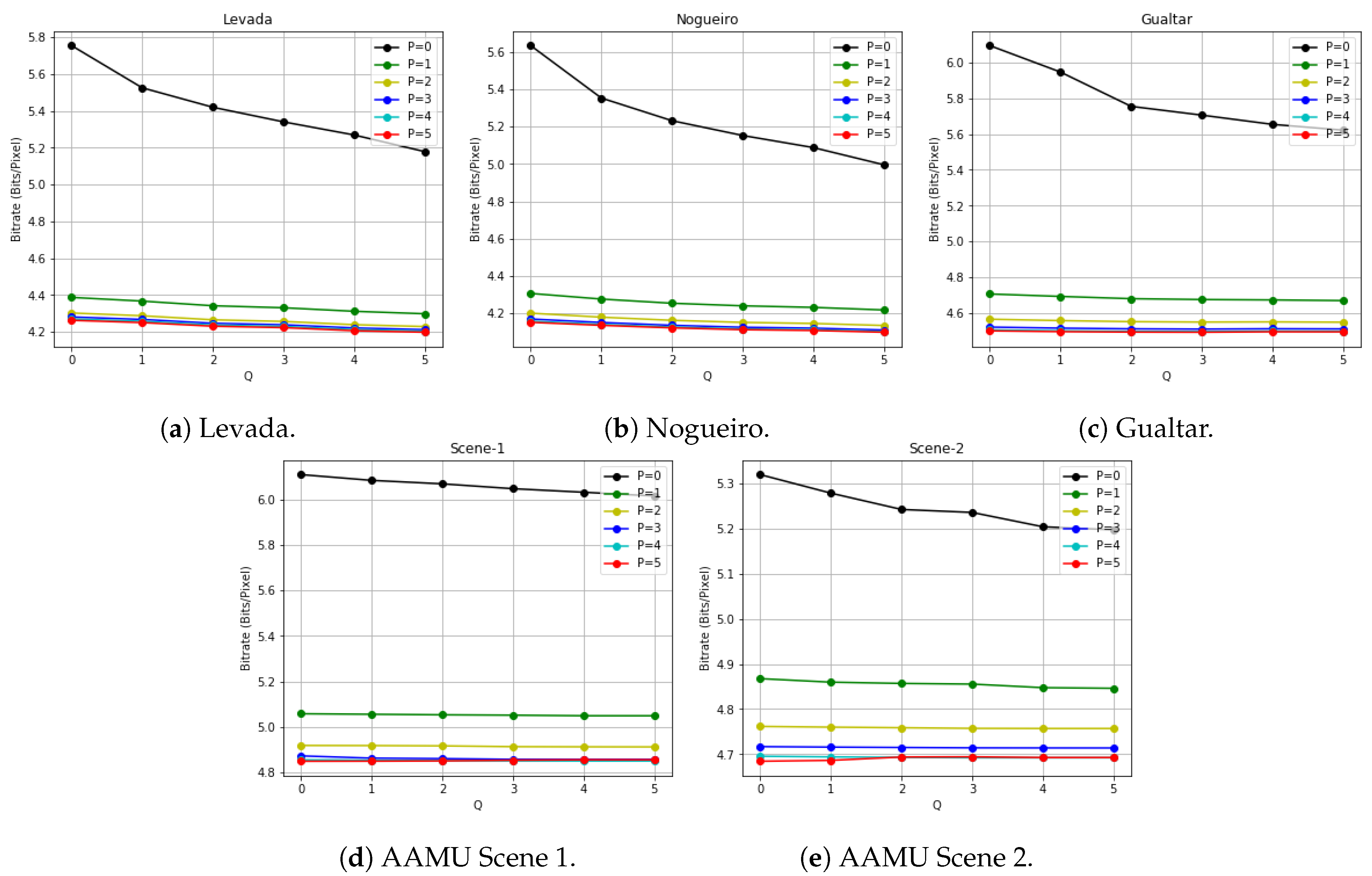
We applied this estimation algorithm on five multitemporal HSI datasets to estimate the potential compression performance of multitemporal hyperspectral image with a combination of various spectral and temporal bands. H ( p , q ) is the entropy conditioned to p previous bands at the current time point and q bands at current spectral band but from previous time points for prediction. Using the binary-source based estimation method, we summed up the conditional entropies of all the bit-planes (a total of 12 bit-planes for all our datasets) as the estimation of H ( p , q ) for each band of the dataset. Then the averages of H ( p , q ) over all bands are reported in Figure 4 for all five datasets. Due to limited space, we only show results for parameters p and q chosen between 0 and 5. More detailed results for other datasets can be found in Table A1, Table A2, Table A3, Table A4 and Table A5 in Appendix A.
From Figure 4, we can observe that as either p or q increases, the general trend is that the conditional entropy decreases; however, as p or q further increases (e.g, from 4 to 5), the reduction of entropy becomes smaller than the case of either p or q going from 0 to 1. This means that including a few previous bands either spectrally or temporally in the context can be very useful to improving the performance of the prediction-based compression algorithms, but the return of adding more bands from distant past will diminish as the correlations get weaker, let alone the increased computational cost associated with involving excessive number of bands for prediction. In addition, the conditional entropy tends to decrease faster with an increased p than with an increased 
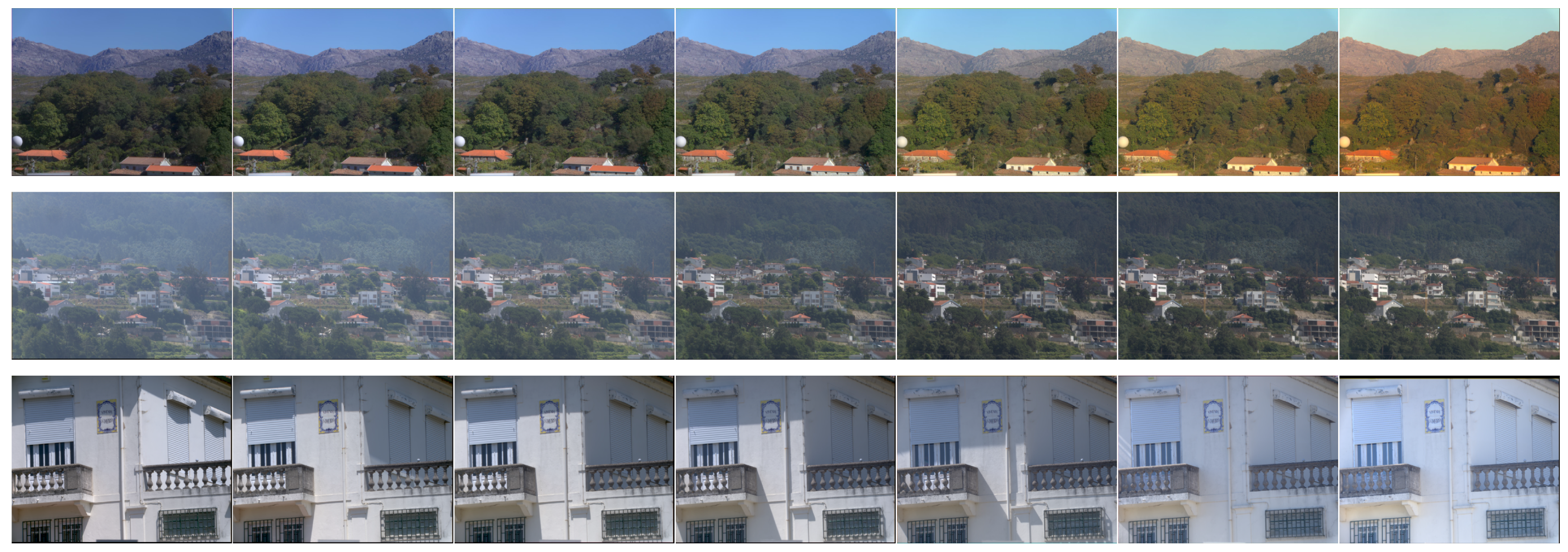
q. This is indicative of stronger spectral correlations than temporal correlations. For example, the fourth image in the first row of Figure 3 represents a dramatic change of illumination conditions during image capturing, thereby weakening the temporal correlations. However, there still exist significant temporal correlations which, if exploited properly, can lead to improved compression by considering only spectral correlations. To this end, we propose a compression algorithm, which exploits temporal correlations in multitemporal HSI data to enhance the overall compression performance.

4. Proposed Algorithm

Our lossless compression algorithm is based on predicting the pixels to be coded, by using a linear combination of those pixels already coded (in a neighboring causal context). Prediction residuals are obtained by subtracting the actual pixel values from their estimates. The residuals are then encoded using entropy coders.
For multitemporal hyperspectral image, the estimate of a pixel value can be obtained by
x ^ p , q j , t = w j , t T y p , q j , t .
where x ^ p , q j , t represents an estimate of a pixel, x p , q j , t , at spatial location ( p , q ) , the jth band and the tth time point, while w j , t denotes the weights for linearly combining the pixel values y p , q j , t . These pixels are drawn from a causal context of several previously coded bands either at the same time point or at previous time points. More specifically, y p , q j , t = x p , q j m , t , x p , q j , t n , m { 1 , 2 , , N b } , n { 1 , 2 , , N t } .
For accurate prediction, weights should be able to adapt to locally changing statistics of pixel values in the multitemporal HSI data. For this sake, learning algorithms were introduced for lossless compression of 3D HSI data [22,32]. Adaptive learning was also used in the so-called Fast Lossless (FL) method. Due to its low-complexity and effectiveness, the FL method has been selected as a new compression standard for multispectral and hyperspectral data by CCSDS (Consultative Committee for Space Data Systems) [23]. The core learning algorithm of the FL method is the sign algorithm, which is a variant of least mean square (LMS). In prior work, we proposed another LMS variant, called correntropy based LMS (CLMS) algorithm, which uses the Maximum Correntropy Criterion [6,8] for lossless compression of 3D and multi-temporal HSI data. By replacing the cost function for LMS based learning with correntropy [33], the CLMS method introduces a new term in the weight update function, which allows the learning rate to change, in order to improve on the conventional LMS based method with a constant learning rate. However, good performance of the CLMS method depends heavily on proper tuning of the kernel variance, which is an optimization parameter used by the “kernel trick” associated with the correntropy. To avoid the excessive need to tune the kernel variance for various types of images in the multitemporal HSI datasets, we adopted the sign algorithm used by the FL predictor with an expanded context vector.
In order to exploit spatial correlations also found in hyperspectral datasets, we follow the simple approach in [22], where local-mean-removed pixel values are used as input to our linear predictor. Specifically, for an arbitrary pixel x p , q j , t in a multi-temporal HSI, the spatial local mean is
μ p , q j , t = [ x p 1 , q 1 j , t + x p 1 , q j , t + x p , q 1 j , t ] / 3 .
After mean subtraction, the causal context becomes
U p , q j , t = x p , q j m , t μ p , q j m , t , x p , q j , t n μ p , q j , t n ,
where m { 1 , 2 , , N b } , and n { 1 , 2 , , N t } . To simplify the notation, we represent the spatial location ( p , q ) with a single index, k, in that k = ( p 1 ) * N y + q , where N y refers to number of pixels in each row within one band. In other words, we line up the pixels in a 1D vector, where the pixels will be processed sequentially in the iterative optimization process of the sign algorithm. Now the predicted value for an arbitrary pixel in each band of multi-temporal HSI dataset is given by
x ^ k j , t = μ k j , t + w j , t T U k j , t ,
where w j , t T are the weights to be adapted sequentially for each band. If follows that the prediction residual can be obtained as
e k j , t = x k j , t x ^ k j , t = x k j , t μ k j , t + w j , t T U k j , t .
We apply the sign algorithm to iteratively update the weights as
w j , t k + 1 = w j , t k + ρ ( k ) · sign ( e k j , t ) · U k j , t ,
where ρ ( k ) is an adaptive learning rate proposed in [23] to achieve fast convergence to solutions close to the global optimum. Our study found that using this adaptive learning rate can provide good results on multitemporal datasets. Note that we need to reset the weights and learning rate for each new band in the dataset to account for potentially varying statistics.
After prediction, all the residuals are mapped to non-negative values [23] and then coded into bitstream losslessly by using the Golomb-Rice Codes (GRC) [34]. Although GRC is selected as the entropy coder because of its computational efficiency [35], we observed that using arithmetic coding can offer slightly lower bitrates, albeit at a much higher computational cost. Pseudo Algorithm 1 of this 4D extension of Fast-Lossless is given to better show its structure and workflow.
Algorithm 1 Fast-Lossless-4D Predictor
  • Input:
  • 1) 4D HSI data X .
  • 2) T (Total # of time frames of X ).
  • 3) B (Total # of spectral bands for each time frame of X )
  • 4) P (# of previous spectral bands).
  • 5) Q (# of bands from previous time frames).
  • 6) μ (learning rate).
  • for t = 1:T do
  •     for b = 1:B do
  •         Local mean subtracted data U using Equations (6) and (7).
  •         initialize: w j , t = 0 .
  •         for each pixel in this band in raster scan order do
  •            Output residual e j , t using Equation (9).
  •            Updating w j , t using Equation (10).
  •         end for
  •     end for
  • end for

5. Simulation Results

We tested the proposed algorithm on all five multitemporal HSI datasets (Levada, Gualtar, Nogueiro, AAMU scene_1 and AAMU scene_2). To show the performance of our algorithm, we present the bitrates after compression in Figure 5 (Detailed results can be found in Table A6, Table A7, Table A8, Table A9 and Table A10). Similar to the conditional entropy estimation results in Section 3, the bitrates were obtained by using various combinations of p (spectral) and q (temporal) number of bands for causal contexts.
We can see that for the case of p = 0 and q = 0 , where we simply use mean subtraction (for spatial decorrelation) without spectral and temporal decorrelation, we can already achieve significant amount of compression on the input data by lowering the original bitrate from 12 bits/pixel to about 6 bits/pixel. If we consider either spectral or temporal correlations, or both, we can achieve additional compression gains on multitemporal HSI data. For example, the bit rate can be reduced by approximately 1 bit/pixel or 0.2 bit/pixel by including in the prediction context one more previous band spectrally or temporally. Generally, the bitrates decrease with more bands being included in the context, which agrees well with the results on condition entropy estimation in Section 3. Furthermore, if we fix the p value and increase the q value, and vice versa, we can achieve better compression. However, the return on including more bands will diminish gradually as p and q further increase. In some cases, we can even have less compression if the context includes some remote bands that might be weakly correlated with the pixels to be predicted. For example, in Table A7, when p = 5 and q = 4 , the corresponding bit rate is 4.4953 , which is 0.0026 higher than 4.4927 (when p = 5 and q = 3 ). Similar examples can be found in Table A9 (when p = 5 and q = 4 ) and in Table A10 (when p = 5 and q = 1 ). Including weakly correlated or totally uncorrelated pixels might lower the quality of the context, leading to degraded compression performance. In this same spirit, we can see that spectral decorrelation turns out to be more effective in reducing the bitrates than temporal decorrelation. This means that spectral correlations are stronger than temporal correlations in the datasets we tested. The reason can be that each hyperspectral image cube in these multitemporal HSI datasets was captured at time intervals of at least a few minutes, during which significant change of pixel values (e.g, caused by illumination condition changes) might have taken place. If the image capturing time interval is reduced, then we expect the stronger temporal correlations.
On the other hand, prediction using only one previous spectral band, and/or the same spectral band but from previous time instance can offer a low-complexity compressor with sufficiently good compression performance. The bitrate results show the wide range of tradeoffs for us to explore in order to balance compression performance with computational complexity.
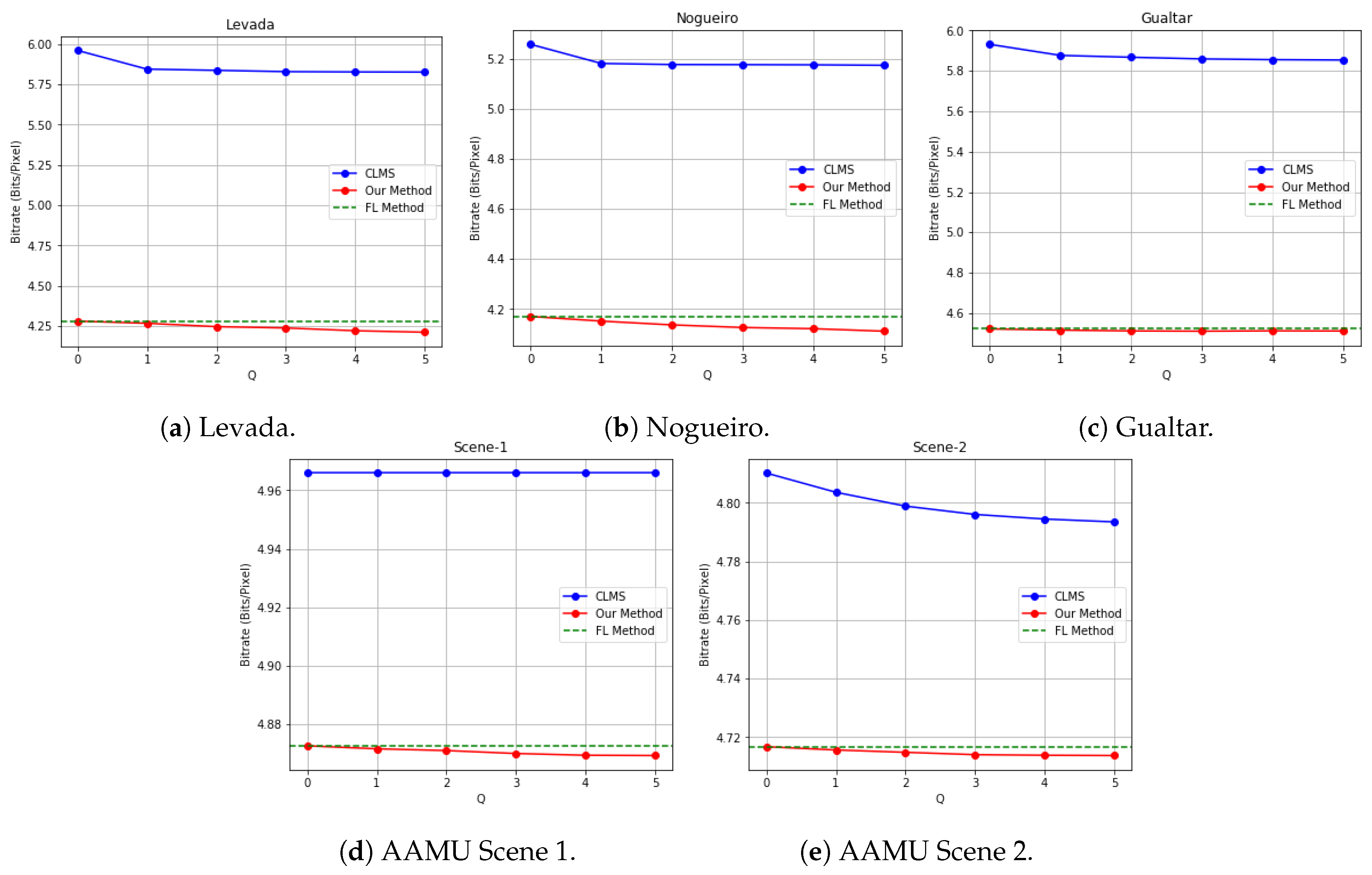
We also compared the proposed algorithm (based on Fast-Lossless algorithm) with our previous work (based on correntropy LMS learning) in [6], namely CLMS, which seems to be the only existing work on lossless compression of multitemporal HSI data. For fair comparison, we use the same parameter setting in [6]. Although it would be straightforward to show the bitrates for both algorithms in multiple tables, we choose to visualize bitrates changes as number of previous bands or number of previous time frames increases for both algorithms. To reduce the complexity of this visualization, we only present P = 3 case since it is the default setting in the FL method. Figure 6 shows the bitrate changes for the five datasets. Note that when Q = 0 , our method is essentially equivalent to 3D FL method. Therefore, we use green dashed line to mark FL method performance in Figure 6. While blue, green and red curves represent CLMS, FL method and ours respectively, it is clear that our methods produce the lowest bitrates consistently. Although bitrates of our method was only slightly lower than applying FL method directly to each one of time framed HSI, it outperformed CLMS method by a significant margin. The improvements on time-lapse datasets are more significant than on AAMU datasets in general. Consistent with results shown previously, we have higher compression gains in the spectral dimension than the temporal dimension. However, the results show that our algorithm can take advantage of the temporal correlations available to bring additional improvements on the overall compression performance.

6. Conclusions

We have proposed a new predictive lossless compression algorithm for multitemporal time-lapse hyperspectral image data using a low-complexity sign algorithm with an expanded prediction context. Simulation results have demonstrated the outstanding capability of this algorithm to compress multitemporal HSI data through spectral and temporal decorrelation. The actual compression results are congruent with the information theoretic analysis and estimation based on conditional entropy. We show that increasing the number of previous bands for prediction can yield better compression performance, by exploiting the spectral and temporal correlations in the datasets.
As future work, we intend to study how to adaptively select bands to build an optimal context vector for prediction. Also, we will investigate how to fully integrate the proposed algorithm and the analytic framework to achieve real-time compression on streaming hyperspectral data. Furthermore, the proposed algorithm can be extended to lossless compression of regions-of-interest in hyperspectral images, which can offer much higher compression than compressing the entire hyperspectral image dataset.

Author Contributions

Conceptualization, H.S. and W.D.P.; Methodology, H.S. and W.D.P.; Software, H.S.; Validation, H.S., Z.J., and W.D.P.; Formal Analysis, H.S.; Investigation, H.S.; Resources, H.S. and W.D.P.; Data Curation, H.S.; Writing-Original Draft Preparation, H.S.; Writing-Review & Editing, H.S., Z.J. and W.D.P.; Visualization, H.S.; Supervision, W.D.P.; Project Administration, W.D.P.; Funding Acquisition, W.D.P.

Funding

This research received no external funding.

Acknowledgments

We would like to thank Joel Fu of the Computer Science Program, Alabama A&M University, Normal, AL, for providing facilities including a SOC 700 hyperspectral camera for data collection in this research.

Conflicts of Interest

The authors declare no conflict of interest.

Appendix A. Condition Entropy Estimation Empirical Experimental Results

Table A1. Conditional entropies H ( p , q ) (bits/pixels), computed for various values of p and q, over “Levada”.
p q = 0 q = 1 q = 2 q = 3 q = 4 q = 5
010.25589.51209.39059.30229.22799.1827
18.76758.46738.37448.31418.26638.2366
28.59518.30638.21928.16338.11798.0895
38.46138.17828.09498.04107.99797.9719
48.34408.07077.99087.93947.89847.8742
58.24147.97337.89777.84977.81137.7888
Table A2. Conditional entropies H ( p , q ) (bits/pixels), computed for various values of p and q, over “Gualtar”.
p q = 0 q = 1 q = 2 q = 3 q = 4 q = 5
010.813710.605710.405710.326610.281810.2387
19.05508.96578.90078.86388.83938.8176
28.83888.75538.69718.66238.63748.6155
38.71078.62838.57158.53628.51008.4870
48.63758.55348.49648.45928.43108.4064
58.58378.49568.43718.39758.36708.3406
Table A3. Conditional entropies H ( p , q ) (bits/pixels), computed for various values of p and q, over “Nogueiro”.
p q = 0 q = 1 q = 2 q = 3 q = 4 q = 5
09.71679.33819.23149.16419.10239.0740
18.24008.11058.06198.03048.00647.9918
28.11657.98907.93957.90807.88417.8695
38.03437.90977.86037.82927.80547.7904
47.97227.84977.80057.76957.74537.7299
57.92007.79797.74927.71807.69367.6775
Table A4. Conditional entropies H ( p , q ) (bits/pixels), computed for various values of p and q, over “Scene-1”.
p q = 0 q = 1 q = 2 q = 3 q = 4 q = 5
08.77857.86247.70557.62717.58347.5548
17.15386.90376.83986.80706.78366.7671
27.04916.81666.75556.72336.69996.6829
36.98396.75996.70036.66836.64486.6272
46.91906.70526.64756.61606.59236.5736
56.85336.65136.59566.56466.54026.5193
Table A5. Conditional entropies H ( p , q ) (bits/pixels), computed for various values of p and q, over “Scene-2”.
p q = 0 q = 1 q = 2 q = 3 q = 4 q = 5
08.13677.50827.36547.31947.27877.2397
16.92486.71096.64666.62026.59556.5719
26.78976.60046.54216.51696.49456.4731
36.71266.53626.48126.45686.43546.4148
46.64616.48106.42896.40526.38436.3637
56.58926.43346.38366.36016.33906.3173
Table A6. Bit rates (bits/pixels), obtained for various values of p and q, on “Levada”.
p q = 0 q = 1 q = 2 q = 3 q = 4 q = 5
05.75385.52485.41935.34005.26895.1784
14.38764.36744.34224.33134.31224.2987
24.30294.28784.26604.25704.23954.2293
34.28134.26794.24714.23894.22184.2125
44.27044.25784.23774.22984.21314.2043
54.26314.25084.23124.22354.20704.1985
Table A7. Bit rates (bits/pixels) obtained for various values of p and q, on “Gualtar”.
p q = 0 q = 1 q = 2 q = 3 q = 4 q = 5
06.09415.94635.75475.70575.65415.6218
14.70644.69284.68024.67544.67324.6695
24.56554.55774.55184.54954.55054.5487
34.52144.51554.51174.51024.51214.5113
44.50574.50064.49774.49664.49904.4984
54.50044.49604.49364.49274.49534.4948
Table A8. Bit rates (bits/pixels), obtained for various values of p and q, on “Nogueiro”.
p q = 0 q = 1 q = 2 q = 3 q = 4 q = 5
05.63295.35245.23125.15215.08744.9953
14.30704.27694.25454.24074.23244.2186
24.20134.18004.16314.15204.14634.1355
34.17014.15154.13644.12604.12124.1112
44.15864.14134.12724.11714.11274.1031
54.15254.13634.12284.11314.10884.0994
Table A9. Bit rates (bits/pixels), obtained for various values of p and q, on “AAMU Scene-1”.
p q = 0 q = 1 q = 2 q = 3 q = 4 q = 5
06.10976.08446.06916.04786.03226.0156
15.05805.05575.05345.05185.04925.0491
24.91864.91814.91684.91334.91264.9122
34.87274.87174.87114.87014.86954.8694
44.85554.85374.85174.85074.85024.8501
54.84914.84954.85064.85384.85564.8556
Table A10. Bit rates (bits/pixels), obtained for various values of p and q, on “AAMU Scene-2”.
p q = 0 q = 1 q = 2 q = 3 q = 4 q = 5
05.32025.27915.24295.23635.20455.1977
14.86754.85974.85694.85544.84754.8461
24.76154.75994.75864.75724.75694.7569
34.71674.71564.71484.71404.71384.7137
44.69534.69394.69284.69204.69194.6920
54.68424.68624.69364.69404.69254.6925
References

References

  1. Shen, H.; Pan, W.D.; Wu, D. Predictive Lossless Compression of regions-of-interest in Hyperspectral Images With No-Data Regions. IEEE Trans. Geosci. Remote Sens. 2017, 55, 173–182. [Google Scholar] [CrossRef]
  2. Thouvenin, P.A.; Dobigeon, N.; Tourneret, J.Y. A Hierarchical Bayesian Model Accounting for Endmember Variability and Abrupt Spectral Changes to Unmix Multitemporal Hyperspectral Images. IEEE Trans. Comput. Imag. 2018, 4, 32–45. [Google Scholar] [CrossRef] [Green Version]
  3. Marinelli, D.; Bovolo, F.; Bruzzone, L. A novel change detection method for multitemporal hyperspectral images based on a discrete representation of the change information. In Proceedings of the 2017 IEEE International Geoscience and Remote Sensing Symposium (IGARSS), Fort Worth, TX, USA, 23–28 July 2017; pp. 161–164. [Google Scholar]
  4. Liu, S.; Bruzzone, L.; Bovolo, F.; Du, P. Unsupervised Multitemporal Spectral Unmixing for Detecting Multiple Changes in Hyperspectral Images. IEEE Trans. Geosci. Remote Sens. 2016, 54, 2733–2748. [Google Scholar] [CrossRef]
  5. Ertürk, A.; Iordache, M.D.; Plaza, A. Sparse Unmixing-Based Change Detection for Multitemporal Hyperspectral Images. IEEE J. Sel. Top. Appl. Earth Obs. 2016, 9, 708–719. [Google Scholar] [CrossRef]
  6. Shen, H.; Pan, W.D.; Dong, Y. Efficient Lossless Compression of 4D Hyperspectral Image Data. In Proceedings of the 3rd International Conference on Advances in Big Data Analytics, Las Vegas, NV, USA, 25–28 July 2016. [Google Scholar]
  7. Zhu, W.; Du, Q.; Fowler, J.E. Multitemporal Hyperspectral Image Compression. IEEE Geosci. Remote Sens. Lett. 2011, 8, 416–420. [Google Scholar] [CrossRef] [Green Version]
  8. Shen, H.; Pan, W.D. Predictive lossless compression of regions-of-interest in hyperspectral image via Maximum Correntropy Criterion based Least Mean Square learning. In Proceedings of the 2016 IEEE International Conference on Image Processing (ICIP), Phoenix, AZ, USA, 25–28 September 2016; pp. 2182–2186. [Google Scholar]
  9. Liaghati, A.; Pan, W.D.; Jiang, Z. Biased Run-Length Coding of Bi-Level Classification Label Maps of Hyperspectral. IEEE J. Sel. Top. Appl. Earth Obs. Remote Sens. 2017, 10, 4580–4588. [Google Scholar] [CrossRef]
  10. Weinberger, M.J.; Seroussi, G.; Sapiro, G. The LOCO-I lossless image compression algorithm: Principles and standardization into JPEG-LS. IEEE Trans. Image Process. 2000, 9, 1309–1324. [Google Scholar] [CrossRef]
  11. Wu, X.; Memon, N. Context-based lossless interband compression-extending CALIC. IEEE Trans. Image Process. 2000, 9, 994–1001. [Google Scholar]
  12. Magli, E.; Olmo, G.; Quacchio, E. Optimized onboard lossless and near-lossless compression of hyperspectral data using CALIC. IEEE Trans. Geosci. Remote Sens. 2004, 1, 21–25. [Google Scholar] [CrossRef]
  13. Wu, X.; Memon, N. Context-based, adaptive, lossless image coding. IEEE Trans. Commun. 1997, 45, 437–444. [Google Scholar] [CrossRef]
  14. Mielikainen, J. Lossless compression of hyperspectral images using lookup tables. IEEE Signal Process. Lett. 2006, 13, 157–160. [Google Scholar] [CrossRef]
  15. Rizzo, F.; Carpentieri, B.; Motta, G.; Storer, J.A. Low-complexity lossless compression of hyperspectral imagery via linear prediction. IEEE Signal Process. Lett. 2005, 12, 138–141. [Google Scholar] [CrossRef]
  16. Wang, H.; Babacan, S.D.; Sayood, K. Lossless Hyperspectral-Image Compression Using Context-Based Conditional Average. IEEE Trans. Geosci. Remote Sens. 2007, 45, 4187–4193. [Google Scholar] [CrossRef] [Green Version]
  17. Said, A.; Pearlman, W.A. A new, fast, and efficient image codec based on set partitioning in hierarchical trees. IEEE Trans. Circuits Syst. Video Technol. 1996, 6, 243–250. [Google Scholar] [CrossRef]
  18. Pearlman, W.A.; Islam, A.; Nagaraj, N.; Said, A. Efficient, low-complexity image coding with a set-partitioning embedded block coder. IEEE Trans. Circuits Syst. Video Technol. 2004, 14, 1219–1235. [Google Scholar] [CrossRef]
  19. Aiazzi, B.; Alparone, L.; Baronti, S.; Lastri, C. Crisp and Fuzzy Adaptive Spectral Predictions for Lossless and Near-Lossless Compression of Hyperspectral Imagery. IEEE Geosci. Remote Sens. Lett. 2007, 4, 532–536. [Google Scholar] [CrossRef]
  20. Mielikainen, J.; Huang, B. Lossless Compression of Hyperspectral Images Using Clustered Linear Prediction with Adaptive Prediction Length. IEEE Geosci. Remote Sens. Lett. 2012, 9, 1118–1121. [Google Scholar] [CrossRef]
  21. Wu, J.; Kong, W.; Mielikainen, J.; Huang, B. Lossless Compression of Hyperspectral Imagery via Clustered Differential Pulse Code Modulation with Removal of Local Spectral Outliers. IEEE Signal Process. Lett. 2015, 22, 2194–2198. [Google Scholar] [CrossRef]
  22. Klimesh, M. Low-Complexity Lossless Compression of Hyperspectral Imagery via Adaptive Filtering; The Interplanetary Network Progress Report; NASA Jet Propulsion Laboratory (JPL): Pasadena, CA, USA, 2005; pp. 1–10. [Google Scholar]
  23. Lossless Multispectral & Hyperspectral Image Compression CCSDS 123.0-B-1, Blue Book, May 2012. 2015. Available online: https://public.ccsds.org/Pubs/123x0b1ec1.pdf (accessed on 10 August 2018).
  24. Mamun, M.A.; Jia, X.; Ryan, M. Sequential multispectral images compression for efficient lossless data transmission. In Proceedings of the 2010 Second IITA International Conference on Geoscience and Remote Sensing, Qingdao, China, 28–31 August 2010; Volume 2, pp. 615–618. [Google Scholar]
  25. Muñoz-Gomez, J.; Bartrina-Rapesta, J.; Blanes, I.; Jimenez-Rodriguez, L.; Aulí-Llinàs, F.; Serra-Sagristà, J. 4D remote sensing image coding with JPEG2000. Proc. SPIE 2010, 7810, 1–9. [Google Scholar]
  26. Ricci, M.; Magli, E. On-board lossless compression of solar corona images. In Proceedings of the 2015 IEEE International Geoscience and Remote Sensing Symposium (IGARSS), Milan, Italy, 26–31 July 2015; pp. 2091–2094. [Google Scholar]
  27. Mamun, M.; Jia, X.; Ryan, M.J. Nonlinear Elastic Model for Flexible Prediction of Remotely Sensed Multitemporal Images. IEEE Geosci. Remote Sens. Lett. 2014, 11, 1005–1009. [Google Scholar] [CrossRef]
  28. Foster, D.H.; Amano, K.; Nascimento, S.M. Time-lapse ratios of cone excitations in natural scenes. Vision Res. 2016, 120, 45–60. [Google Scholar] [CrossRef] [PubMed]
  29. SOC700 Series Hyperspectral Imaging Systems. 2018. Available online: https://surfaceoptics.com/products/hyperspectral-imaging/soc710-portable-hyperspectral-camera/ (accessed on 10 August 2018).
  30. Time-Lapse Hyperspectral Radiance Images of Natural Scenes 2015. 2015. Available online: http://personalpages.manchester.ac.uk/staff/david.foster/Time-LapseHSIs/Time-LapseHSIs2015.html (accessed on 1 March 2015).
  31. Magli, E. Multiband Lossless Compression of Hyperspectral Images. IEEE Trans. Geosci. Remote Sens. 2009, 47, 1168–1178. [Google Scholar] [CrossRef] [Green Version]
  32. Shen, H.; Pan, W.D.; Wang, Y. A Novel Method for Lossless Compression of Arbitrarily Shaped Regions of Interest in Hyperspectral Imagery. In Proceedings of the 2015 IEEE SoutheastCon, Fort Lauderdale, FL, USA, 9–12 April 2015; pp. 1–6. [Google Scholar]
  33. Liu, W.; Pokharel, P.P.; Principe, J.C. Correntropy: Properties and Applications in Non-Gaussian Signal Processing. IEEE Trans. Signal Process. 2007, 55, 5286–5298. [Google Scholar] [CrossRef]
  34. Golomb, S. Run-length encodings (Corresp.). IEEE Trans. Inf. Theory 1966, 12, 399–401. [Google Scholar] [CrossRef]
  35. Shen, H.; Pan, W.D.; Dong, Y.; Jiang, Z. Golomb-Rice Coding Parameter Learning Using Deep Belief Network for Hyperspectral Image Compression. In Proceedings of the IEEE International Geoscience and Remote Sensing Symposium (IGARSS), Fort Worth, TX, USA, 23–28 July 2017; pp. 2239–2242. [Google Scholar]
Figure 1. A multitemporal hyperspectral image dataset, where X and Y are the spatial directions, Z is the spectral direction, and T is the temporal direction.
Jimaging 04 00142 g001
Figure 2. Some sample images at different time instants from the time-lapse hyperspectral image datasets (from top to bottom: Levada, Nogueiro and Gualtar).
Jimaging 04 00142 g002
Figure 3. Sample images at different time instants from the AAMU hyperspectral image datasets (top: Scene-1, and bottom: Scene-2).
Jimaging 04 00142 g003
Figure 4. Conditional entropies over five datasets for different P and Q combination.
Jimaging 04 00142 g004
Figure 5. Bitrates over five datasets for different P and Q combination.
Jimaging 04 00142 g005
Figure 6. Bitrates comparison with CLMS and FL methods over five datasets for different Q when P = 3 .
Jimaging 04 00142 g006
Table 1. Multitemporal hyperspectral image datasets.
DatasetSizeThe Number of Time FramesPrecision (bits)
Levada 1024 × 1344 × 33 712
Gualtar 1024 × 1344 × 33 912
Noguerio 1024 × 1344 × 33 912
Scene-1 640 × 640 × 120 2112
Scene-2 640 × 640 × 120 1612

