Two-Dimensional Orthonormal Tree-Structured Haar Transform for Fast Block Matching

Abstract

The goal of block matching (BM) is to locate small patches of an image that are similar to a given patch or template. This can be done either in the spatial domain or, more efficiently, in a transform domain. Full search (FS) BM is an accurate, but computationally expensive procedure. Recently introduced orthogonal Haar transform (OHT)-based BM method significantly reduces the computational complexity of FS method. However, it cannot be used in applications where the patch size is not a power of two. In this paper, we generalize OHT-based BM to an arbitrary patch size, introducing a new BM algorithm based on a 2D orthonormal tree-structured Haar transform (OTSHT). Basis images of OHT are uniquely determined from the full balanced binary tree, whereas various OTSHTs can be constructed from any binary tree. Computational complexity of BM depends on a specific design of OTSHT. We compare BM based on OTSHTs to FS and OHT (for restricted patch sizes) within the framework of image denoising, using WNNM as a denoiser. Experimental results on eight grayscale test images corrupted by additive white Gaussian noise with five noise levels demonstrate that WNNM with OTSHT-based BM outperforms other methods both computationally and qualitatively.

1. Introduction

Block matching (BM) is a fundamental method to locate small patches in an image that match a given patch which is referred to as a template. It has many practical applications, such as object detection [1], object tracking [2], image registration [3], and image analysis [4,5], to name few. Block matching requires the vast computations due to a large search space involving many potential candidates. Full search (FS) algorithm is generally most accurate BM, in which the similarity scores of all candidate windows to the template are calculated in a sliding window manner in the spatial domain. To speed up the matching procedure, various fast algorithms have been proposed. They can be classified into the following two main categories: full search equivalent and non full search equivalent algorithms. Full search equivalent algorithms accelerate the BM by pruning many candidate windows that cannot be the best match windows. These algorithms ensure the results of the full search algorithm. Conversely, non full search equivalent algorithms accelerate by limiting the scope of the search space or by using approximated patterns. The results of non full search equivalent algorithms may be different from those of the full search algorithms. Many full search equivalent algorithms have been proposed in literature, see e.g., [6,7]. The BM methods can be also categorized into spatial- and transform-based. Among transform-based methods, decompositions by the rectangular orthogonal bases, such as orthogonal Haar and Walsh, are most studied ones [8,9]. As it was demonstrated in [8], BM in orthogonal Haar transform (OHT) domain appears to be more efficient than BM based on Walsh-Hadamard transform (WHT) [9], Gray-Code kernels(GCK) [10], and incremental dissimilarity approximations (IDA) [7]. One of the reason behind this is the use of the integral image, technique originally proposed by Crow [11] and broadened later by Viola and Jones [12]. Once the integral image is generated, the sum of pixel intensities of a rectangle region in the image can be easily obtained by three operations (two subtractions and one addition), regardless of the size of a region. Thus, as it was demonstrated in [8], integral image can be a useful tool to calculate OHT coefficients, and OHT is efficient especially when the templates size is large. To evaluate the speed-up over FS equivalent methods, a template of size $2^n\times 2^n$ ($n\ge 4$) was considered, with the standard deviation of pixel intensities in the template greater than 45. In [13], it was reported that the algorithm based on OHT was faster than other algorithms, including low resolution pruning (LRP) [14], WHT [9], and fast Fourier transform (FFT).

Despite the above mentioned benefits of OHT-based BM, it has the following drawback - the block size shall be a power of 2, restricting an applicability of OHT-based BM methods, e.g., in nonlocal image restoration [15,16,17,18,19], in which the size of patch is important for the restoration performance. Nonlocal image restoration methods use the fact that there exists a high level of self-similarity (fractal similarity) in natural images, and one can use this for collaborative processing of similar patches extracted from an image. Non-local image denoising method uses BM to collect similar patches and process them collaboratively. The denoising performance directly depends on patches collected in the image. One of the examples of such application is image denoising [15,16,17], where various size of templates (a regions centered at each pixel) are used depending on noise level. For example, non-local mean denoising [15], uses the template size is $7\times 7$ for a moderate noise level; in weighted nuclear norm minimization denoising method [16], templates of sizes $6\times 6$, $7\times 7$, and $8\times 8$ are used.

In the present paper, we propose a specific design of the orthonormal tree-structured Haar transform (OTSHT) for fast BM with an arbitrary size. The one-dimensional OTSHT [20], proposed by one of the authors, has a freedom of the design and meets the requirements of fast BM. We present the mathematical expressions defining 2D OTSHT, construct several types of the two-dimensional OTSHTs including two prime tree structures, and evaluate them as FS equivalent algorithms in terms of speed and pruning performance. In addition, as a non FS equivalent algorithm, we demonstrate the applicability of the proposed OTSHT in the state-of-the-art image denoising. The obtained results demonstrate that the new method is faster and even produces slightly better PSNR than those where FS or OHT are used. This paper extends the results of the initial study, presented in [21,22].

The paper is organized as follows: We present the mathematical expression and concrete basis images of OTSHT for BM in Section 2. The fast BM algorithm using OTSHT is described in Section 3. Our evaluations of the specific designs of OTSHT for BM are detailed in Section 4. The application to image denoising is demonstrated in Section 5. Finally, in Section 6, we conclude our study.

2. Basis Images of Two-Dimensional Orthonormal Tree-Structured Haar Transform for Fast Block Matching

In this section, we consider the basis images of orthonormal Haar transform for fast BM with an arbitrary patch size. To do this, extending the OTSH transforms, introduced in [20], to the 2D and select two extreme cases of these transforms: one based on balanced-binary tree decompositions and the second one on the logarithmic tree decomposition.

2.1. Binary Tree and Interval Subdivision

Two-dimensional orthonormal tree-structured Haar transform is designed by an arbitrary binary tree having N leaves with d depth.

In the binary tree, the topmost node is referred to as a root and the bottom nodes are referred to as the leaves. Each node is labeled by $\alpha$. The labeling process starts from the root. The left and right children of the root are labeled as 0 and 1, respectively. When the node has two children, the left and right children are labeled by adding 0 and 1 to the right end of the precedent node label, respectively.

Let ${\alpha }_0$ and ${\alpha }_1$ be the left and right children of the node $\alpha$, respectively. Let $\nu \left(\alpha \right)$ be the number of leaves that node $\alpha$ has. The interval, $I_{\alpha }$, of node $\alpha$ is defined from the structure of the binary tree. Intervals $I_{root}$, $I_0$, and $I_1$ are defined as

$$\begin{array}{cc}\hfill I_{root}& =[0,1)\hfill \end{array}$$

(1)

$$\begin{array}{cc}\hfill I_0& =\left[0,\frac{\nu \left(0\right)}{\nu \left(root\right)}\right)\hfill \end{array}$$

(2)

$$\begin{array}{cc}\hfill I_1& =\left[\frac{\nu \left(0\right)}{\nu \left(root\right)},1\right).\hfill \end{array}$$

(3)

Otherwise, for $I_{\alpha }=[a,b)$,

$$\begin{array}{c}\hfill I_{{\alpha }_0}=\left[a,a+\frac{\nu \left({\alpha }_0\right)}{\nu \left(\alpha \right)}(b-a)\right)\end{array}$$

(4)

and

$$\begin{array}{c}\hfill I_{{\alpha }_1}=\left[a+\frac{\nu \left({\alpha }_0\right)}{\nu \left(\alpha \right)}(b-a),b\right).\end{array}$$

(5)

Figure 1 shows the binary tree and the interval splitting. The tree has three leaves with depth two. A circle represents a node. The number above the circle is the label and the number in the circle is the number of the leaves that the node has.

2.2. Orthonormal Tree-Structured Haar Transform Basis Images

Label $\beta$ is introduced for the vertical direction in addition to label $\alpha$ for the horizontal direction. A total of $N^2$ basis images of size $N\times N$ are generated from a binary tree having N leaves.

There are four functions for constructing the basis images of OTSHT for BM. The function for regions $(I_{root}\times I_{root})$ is defined as

$$\begin{array}{cc}\hfill {\phi }_0(s,t)& =\begin{array}{cc}\frac{1}{N}& (s,t)\in I_{root}\times I_{root}\end{array}\hfill \end{array}$$

(6)

which is used once to generate the first basis image. Otherwise, for region $(I_{\alpha }\times I_{\beta })$, the following functions are used:

$$\begin{array}{cc}\hfill {\phi }_1(s,t)& =\left\{\begin{array}{cc}\frac{\nu \left({\beta }_1\right)}{\sqrt{\nu \left(\alpha \right)\nu \left(\beta \right)\nu \left({\beta }_0\right)\nu \left({\beta }_1\right)}},& (s,t)\in I_{\alpha }\times J_{{\beta }_0}\\ -\frac{\nu \left({\beta }_0\right)}{\sqrt{\nu \left(\alpha \right)\nu \left(\beta \right)\nu \left({\beta }_0\right)\nu \left({\beta }_1\right)}},& (s,t)\in I_{\alpha }\times J_{{\beta }_1}\\ 0,& \mathrm{otherwise}\end{array}\right.\hfill \end{array}$$

(7)

$$\begin{array}{cc}\hfill {\phi }_2(s,t)& =\left\{\begin{array}{cc}\frac{\nu \left({\alpha }_1\right)}{\sqrt{\nu \left(\alpha \right)\nu \left({\alpha }_0\right)\nu \left({\alpha }_1\right)\nu \left({\beta }_0\right)}},& (s,t)\in I_{{\alpha }_0}\times J_{{\beta }_0}\\ -\frac{\nu \left({\alpha }_0\right)}{\sqrt{\nu \left(\alpha \right)\nu \left({\alpha }_0\right)\nu \left({\alpha }_1\right)\nu \left({\beta }_0\right)}},& (s,t)\in I_{{\alpha }_1}\times J_{{\beta }_0}\\ 0,& \mathrm{otherwise}\end{array}\right.\hfill \end{array}$$

(8)

$$\begin{array}{cc}\hfill {\phi }_3(s,t)& =\left\{\begin{array}{cc}\frac{\nu \left({\alpha }_1\right)}{\sqrt{\nu \left(\alpha \right)\nu \left({\alpha }_0\right)\nu \left({\alpha }_1\right)\nu \left({\beta }_1\right)}},& (s,t)\in I_{{\alpha }_0}\times J_{{\beta }_1}\\ \frac{\nu \left({\alpha }_0\right)}{\sqrt{\nu \left(\alpha \right)\nu \left({\alpha }_0\right)\nu \left({\alpha }_1\right)\nu \left({\beta }_1\right)}},& (s,t)\in I_{{\alpha }_1}\times J_{{\beta }_1}\\ 0,& \mathrm{otherwise}\end{array}\right.\hfill \end{array}$$

(9)

The interval of the nodes of focus is used for generating the positive and negative value regions, where the region is decomposed according to the intervals in the horizontal and vertical directions. Figure 2 illustrates a set of procedures for decomposition of the region when the nodes of focus are $(\alpha ,\beta )$.

A positive value and a negative value regions are represented in white and black, respectively. First, region $(I_{\alpha }\times I_{\beta })$ is vertically divided into two regions $(I_{\alpha }\times I_{{\beta }_0})$ and $(I_{\alpha }\times I_{{\beta }_1})$, and the value at each region is assigned by (7). Then the positive value region $(I_{\alpha }\times I_{{\beta }_0})$ is horizontally divided into two regions $(I_{{\alpha }_0}\times I_{{\beta }_0})$ and $(I_{{\alpha }_1}\times I_{{\beta }_0})$ by (8), while the negative value region is divided into two regions $(I_{{\alpha }_0}\times I_{{\beta }_1})$ and $(I_{{\alpha }_1}\times I_{{\beta }_1})$ by (9).

The nodes of focus start with $(root,root)$. Once the set of procedures is conducted, the nodes of focus are changed to $({\alpha }_0,{\beta }_0)$, $({\alpha }_1,{\beta }_0)$, $({\alpha }_0,{\beta }_1)$, and $({\alpha }_1,{\beta }_1)$. The nodes of focus are changed until all nodes are used. When the region is indivisible, i.e., $\nu \left(\alpha \right)=1$ and $\nu \left(\beta \right)=1$, no more decomposition is applied.

Figure 3 shows the appearance of constructing the set of basis images according to the binary tree shown in Figure 1. A positive, a negative, and zero value regions are represented in white, black, and grey, respectively. The first basis image is given by (6); the second, by (7); the third and forth, by (8) and (9), respectively. The set of procedures is completed and then the nodes of focus are changed. When $(\alpha ,\beta )=(0,0)$, the fifth basis image is given by (7); the seventh and eighth, by (8) and (9), respectively. When $(\alpha ,\beta )=(1,0)$, the sixth basis image is given by (7), but no more decomposition is applied because $\alpha$ has no child, i.e., $\nu \left(\alpha \right)=1$. When $(\alpha ,\beta )=(0,1)$, since $\alpha$ has a child and $\beta$ has no child, i.e., $\nu \left(\alpha \right)>1$ and $\nu \left(\beta \right)=1$. the ninth basis image is given by (8). When $(\alpha ,\beta )=(1,1)$, since both $\alpha$ and $\beta$ do not have any children, no more decomposition is applied. Thus, a total of nine basis images of size $3\times 3$ is generated.

2.3. Balanced Binary Tree and Logarithmic Binary Tree

Tree structured Haar transform has a freedom of the design. We consider two prime tree structures, balanced binary tree and logarithmic binary tree. They are extreme cases.

The balanced binary tree is depth-balanced where the depths of left and right subtrees of each node are within 1. Figure 4a shows an example of the balanced binary tree of the depth 3 having $N=5$ leaves and its intervals.

Figure 4b shows the appearance of the balanced binary tree-based (B-) OTSHT basis images generated by (6) through (9). In the 25 basis images, there are totally $r=11$ rectangles with different sizes: $5\times 5$, $5\times 3$, $5\times 2$, $3\times 3$, $3\times 2$, $3\times 1$, $2\times 3$, $2\times 2$, $2\times 1$, $1\times 2$, and $1\times 1$, having $N_h=4$ different heights: 5, 3, 2, and 1.

The logarithmic binary tree is the special case of the Fibonacci p-tree [20] when $p\to \infty$. Figure 5a shows an example of the logarithmic binary tree of the depth 4 having $N=5$ leaves. Figure 5b shows the appearance of logarithmic binary tree-based (L-) OTSHT basis images generated by (6)–(9). In the set of 25 basis images, there are totally $r=15$ rectangles with the different sizes: $5\times 5$, $5\times 4$, $5\times 1$, $4\times 4$, $4\times 3$, $4\times 1$, $3\times 3$, $3\times 2$, $3\times 1$, $2\times 2$, $2\times 1$, $1\times 4$, $1\times 3$, $1\times 2$, and $1\times 1$, having $N_h=5$ different heights: 5, 4, 3, 2, and 1.

As we have seen, although the number of leaves is the same, the different structures are constructed, which leads to the different number of rectangles. The number of rectangles with different sizes affects the computational complexity.

2.4. Relation between OHT and OTSHT

The OHT is the special case of OTSHT, when the tree for constructing OHT is a full balanced binary tree. Figure 6a,b shows the full binary tree having four leaves and the appearance of generating OHT basis images, respectively.

3. Fast Block Matching Algorithm Using Two-Dimensional Orthonormal Tree-Structured Haar Transform

OTSHT is used for both FS-equivalent fast BM algorithm and non FS-equivalent one. In both algorithms, the similarity of all candidate patches to the template is calculated by SSD in the transform domain.

Let ${\mathbf{x}}_j$ be the column vector of the j-th window in a proper order. The k-th OTSHT coefficient, $X_j\left(k\right)$ of ${\mathbf{x}}_j$ is obtained by

$$\begin{array}{c}\hfill X_j\left(k\right)={\mathbf{h}}_k^T{\mathbf{x}}_j\end{array}$$

(10)

where ${\mathbf{h}}_k$ is the column vector of the k-th OTSHT basis image in a proper order. In practice, since the elements of OTSHT basis images have $+1$ and $-1$, forming a rectangle region, the OTSHT coefficient is obtained by just few operations with the integral image [11,12]. Moreover, the strip sum technique reduces the number of operations [8].

3.1. FS-Equivalent Algorithm Using OTSHT

The OTSHT can be used for FS-equivalent algorithm. The fast FS-equivalent algorithm using OHT [8] is applicable to OTSHT. The operations are significantly reduced by iterative pruning process described below.

When an appropriate threshold is used, one may securely reject the windows with sum of squared differences (SSDs) above the threshold: If

$$\begin{array}{c}\hfill \left|\right|{\mathbf{X}}_j^K-{\mathbf{X}}_t^K{\left|\right|}^2>threshold,\end{array}$$

(11)

then the j-th window is rejected from the search, where ${\mathbf{X}}_j^K$ and ${\mathbf{X}}_t^K$ are the OTSHT coefficients including the first to K-th ones, i.e., ${\mathbf{X}}_j^K={[X_j\left(1\right),X_j\left(2\right),\cdots ,X_j\left(K\right)]}^T$, of the j-th window and the template, respectively. Once the window is rejected, neither the OTSHT coefficient nor the SSD of the window is calculated. For each iteration of k, the k-th OTSHT coefficient and the SSDs of the remaining windows are calculated. The iteration is performed until the number of remaining windows is small. Algorithm 1 shows the pseudo code for FS-equivalent algorithm using OTSHT.

Algorithm 1: FS-equivalent BM.

Input: template $\mathbf{t}$ of size $N\times N$ and image $\mathbf{x}$   1: make basis images   2: make the integral image of $\mathbf{x}$   3: initialize a vector $\mathbf{Flg}$ to ‘$true$’   4: for $k=1$: $N^2$   5:       set the k-th OTSHT coefficient of ${\mathbf{x}}_t$ to ${\mathbf{X}}_t\left(k\right)$   6:       for each patch ${\mathbf{x}}_j$ in $\mathbf{x}$   7:             if ${\mathbf{Flg}}_j==‘true’$   8:                   set the k-th OTSHT coefficient of ${\mathbf{x}}_j$ to ${\mathbf{X}}_j\left(k\right)$   9:                   if $\left|\right|{\mathbf{X}}_j^K-{\mathbf{X}}_t^K{\left|\right|}_2^2\ge$ threshold 10:                         ${\mathbf{Flg}}_j=‘false’$ 11:                   end 12:             end 13:       end 14:       if the number of $‘true’$ in $\mathbf{Flg}$ is enough small 15:             break 16:       end 17: end 18: FS in remaining candidates Output: estimated window

3.2. Non FS-Equivalent Algorithm Using OTSHT

The OTSHT can be used for non-FS-equivalent algorithm. Instead of the iterative pruning process of the FS-equivalent algorithm mentioned above, the number of OTSHT basis images is limited for reducing the computational load. The similarity using the first to K-th OTSHT coefficients are calculated at a time. The number K is determined by users. Algorithm 2 shows the pseudo code for non FS-equivalent algorithm using OTSHT.

Algorithm 2: non FS-equivalent BM.

Input: template $\mathbf{t}$ of size $N\times N$ and image $\mathbf{x}$ 1: make basis images 2: make the integral image of $\mathbf{x}$ 3: for $k=1$: K 4:       set the k-th OTSHT coefficient of ${\mathbf{x}}_t$ to ${\mathbf{X}}_t\left(k\right)$ 5:       for each patch ${\mathbf{x}}_j$ in $\mathbf{x}$ 6:             set the k-th OTSHT coefficient of ${\mathbf{x}}_j$ to ${\mathbf{X}}_j\left(k\right)$ 7:       end 8: end 9: estimated window j = ${min}_j$($\left|\right|{\mathbf{X}}_j^K-{\mathbf{X}}_t^K{\left|\right|}_2^2$) Output: estimated window

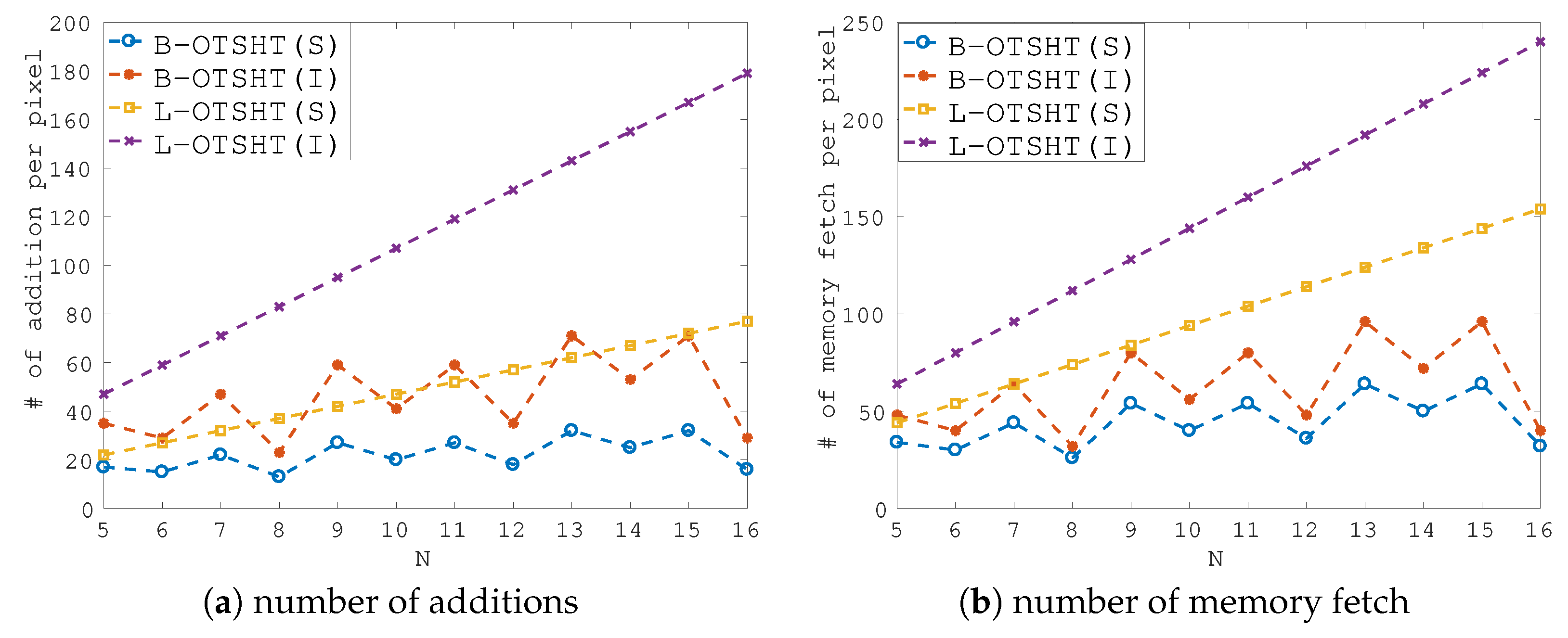
3.3. Computational Complexity

Figure 7a,b shows the number of additions per pixel and the number of memory fetch operations per pixel, respectively, for computing the OTSHT coefficients using strip sum technique [8] (referred to as (S)), and integral image only (referred to as (I)). Compared to the number of operations for OHT (i.e., $N=8$ or $N=16$), the number of additions and memory fetch operations for B-OTSHT coefficients does not gain much, while that for the L-OTSHT is more than double and increases as N increases.

With regard to memory usage, when the width and height of an image are $J_1$ and $J_2$, respectively, and r rectangles having $N_h$ different heights in OTSHT basis images, $J_1{J}_2{N}_h$ memory size will be required for the horizontal strip sum technique [8], $J_1{J}_2$ memory for the integral image, and $J_1{J}_2$ memory for saving the similarity. Therefore, $N_h$ time more memory size is required for the strip sum technique.

Table 1. The number of rectangles, r, with different sizes having different height, $N_h$, and different width, $N_w$, in the set of OTSHT of size $N\times N$.

N	B-OTSHT			L-OTSHT
	r	${\mathit{N}}_{\mathit{h}}$	${\mathit{N}}_{\mathit{w}}$	r	${\mathit{N}}_{\mathit{h}}$	${\mathit{N}}_{\mathit{w}}$
5	11	4	4	15	5	5
6	9	4	4	19	6	6
7	15	5	5	23	7	7
8	7	4	4	27	8	8
9	19	6	6	31	9	9
10	13	5	5	35	10	10
11	19	6	6	39	11	11
12	11	5	5	43	12	12
13	23	7	7	47	13	13
14	17	6	6	51	14	14
15	23	7	7	55	15	15
16	9	5	5	59	16	16

summarizes the number of rectangles with different sizes having different heights and different widths in the set of $N^2$ OTSHT.

4. Experimental Section

In experiments, the fast BM algorithm using OHT and the fast BM algorithm using OTSHT are simply denoted by OHT and OTSHT, respectively, unless otherwise specified. We evaluate OTSHT in comparison to OHT and FS. All experiments are implemented using MATLAB and performed on Macintosh with 4.0 GHz core i7. Eight test images [23] were used for the evaluation.

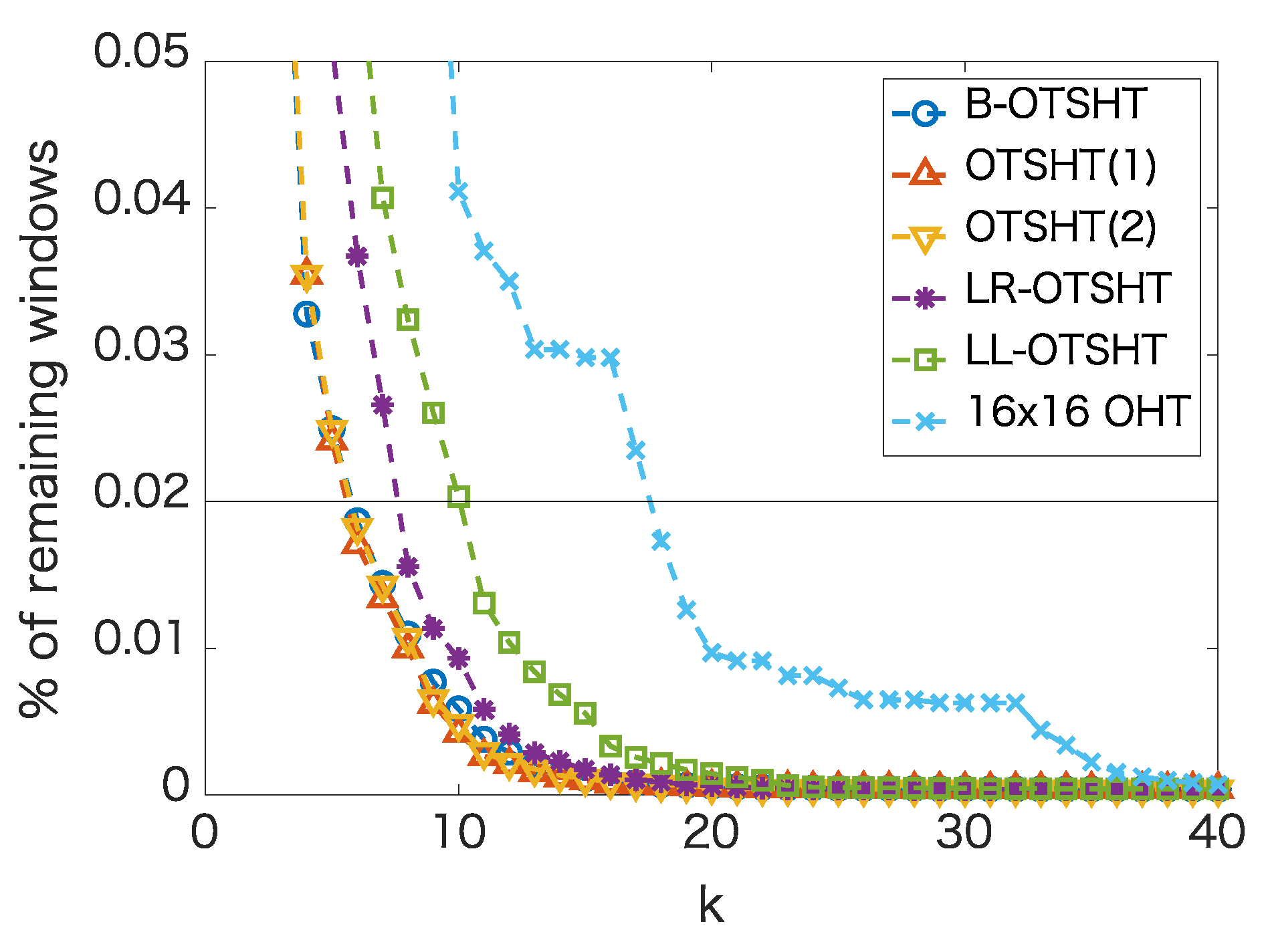
4.1. Pruning Performance of Different Tree Structures

We evaluated the tree structures for the OTSHT basis images. We consider five examples of binary tree having $N=9$ leaves shown in Figure 8.

Figure 8a–e shows examples of a balanced binary tree, a binary tree of depth 4, a binary tree of depth 5, the logarithmic binary tree where all right children are leaves, and the logarithmic binary tree where all left children are leaves, respectively.

Table 2. Number of rectangles of different sizes having different heights of $9\times 9$ OTSHT.

Structure	r	${\mathit{N}}_{\mathit{h}}$	Details
B-OTSHT (Figure 8a)	19	6	$9\times 9$, $5\times 9$, $4\times 9$, $5\times 5$, $5\times 4$, $4\times 5$, $4\times 4$,
			$3\times 5$, $2\times 5$, $3\times 4$, $2\times 4$, $3\times 3$, $3\times 2$, $2\times 3$,
			$2\times 2$, $1\times 3$, $1\times 2$, $2\times 1$, $1\times 1$
OTSHT (1) (Figure 8b)	17	5	$9\times 9$, $6\times 9$, $3\times 9$, $6\times 6$, $6\times 3$, $3\times 6$, $3\times 3$,
			$3\times 2$, $3\times 2$, $3\times 1$, $2\times 6$, $2\times 3$, $2\times 2$, $2\times 1$,
			$1\times 6$, $1\times 3$, $1\times 2$, $1\times 1$
OTSHT (2) (Figure 8c)	25	6	$9\times 9$, $6\times 9$, $6\times 6$, $6\times 3$, $4\times 6$, $4\times 4$, $4\times 3$,
			$4\times 2$, $4\times 1$, $3\times 9$, $3\times 6$, $3\times 4$, $3\times 3$, $3\times 2$,
			$3\times 1$, $2\times 6$, $2\times 4$, $2\times 3$, $2\times 2$, $2\times 1$, $1\times 6$,
			$1\times 4$, $1\times 3$, $1\times 2$, $1\times 1$
LR-OTSHT (Figure 8d)	31	9	$9\times 9$, $8\times 9$, $1\times 9$, $8\times 8$, $8\times 1$, $1\times 8$, $1\times 1$,
			$7\times 8$, $7\times 1$, $1\times 7$, $7\times 7$, $6\times 1$, $1\times 6$, $6\times 7$,
			$5\times 1$, $1\times 5$, $6\times 6$, $4\times 1$, $1\times 4$, $5\times 6$, $3\times 1$,
			$1\times 3$, $5\times 5$, $2\times 1$, $1\times 2$, $4\times 5$, $4\times 4$, $3\times 4$,
			$3\times 3$, $2\times 3$, $2\times 2$
LL-OTSHT (Figure 8e)	31	9	$9\times 9$, $8\times 9$, $1\times 9$, $8\times 8$, $8\times 1$, $1\times 8$, $1\times 1$,
			$7\times 8$, $7\times 1$, $1\times 7$, $7\times 7$, $6\times 1$, $1\times 6$, $6\times 7$,
			$5\times 1$, $1\times 5$, $6\times 6$, $4\times 1$, $1\times 4$, $5\times 6$, $3\times 1$,
			$1\times 3$, $5\times 5$, $2\times 1$, $1\times 2$, $4\times 5$, $4\times 4$, $3\times 4$,
			$3\times 3$, $2\times 3$, $2\times 2$

summarizes the number of rectangles of different sizes having different heights. From the trees shown in Figure 8a–e, we construct the OTSHT basis images, which are referred to as B-OTSHT, OTSHT(1), OTSHT(2), LR-OTSHT, and LL-OTSHT, respectively.

Figure 9 shows the percentage of remaining windows after pruning, which was conducted every k-th basis image. The number is averaged over 100 templates. In this experiment, the performance of OTSHT(1) is only slightly better than that of B-OTSHT and OTSHT(2). On the other hand, the performances of LR-OTSHT and LL-OTSHT were not satisfactory.

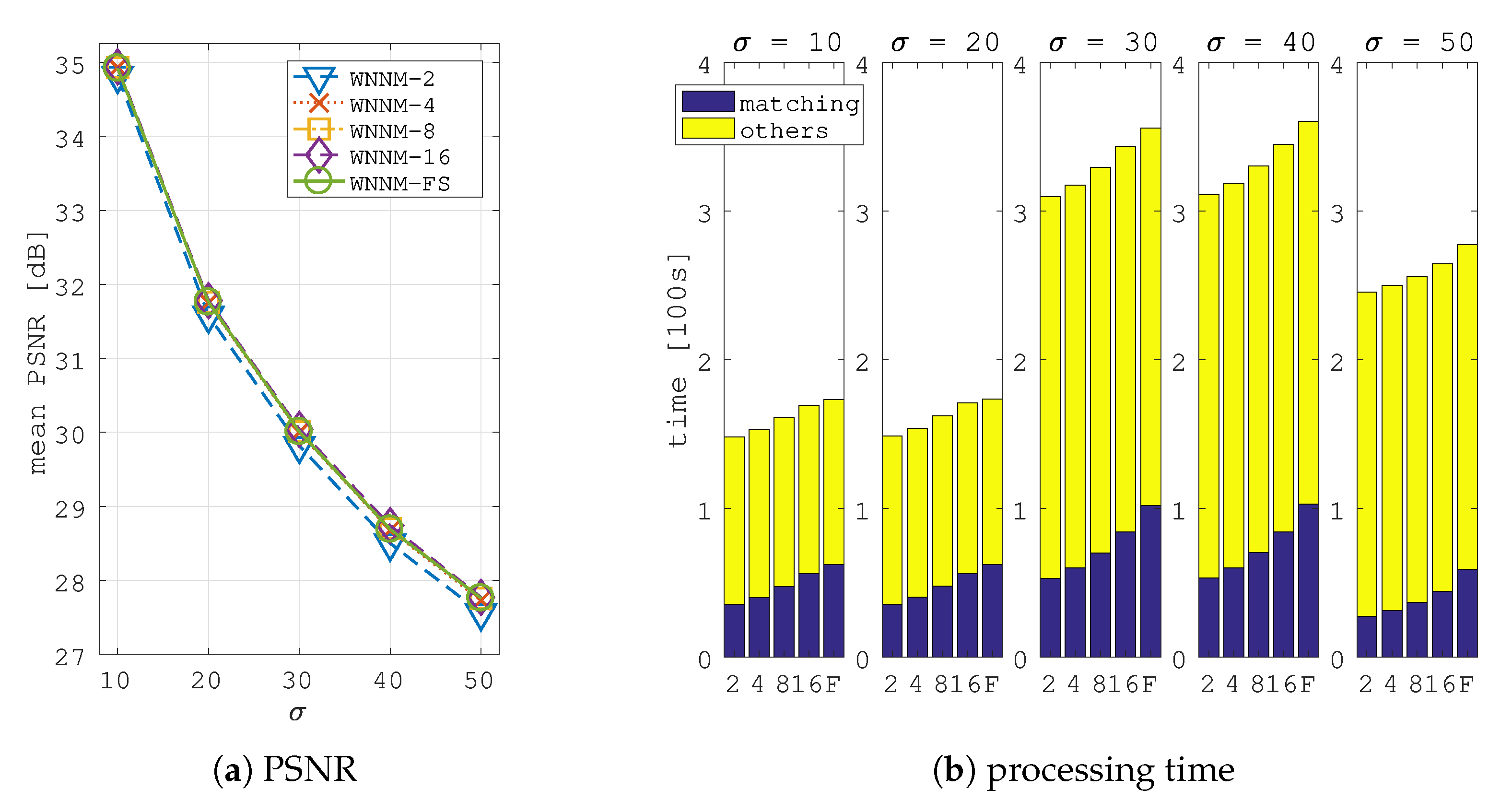
4.2. FS Equivalent Algorithm

We performed OTSHT, OHT and FS for evaluating the processing time. The template size, $N\times N$, was changed from $N=5$ to 15. 100 templates were chosen every 55 pixels in the raster scan. Balanced binary tree is used for constructing OTSHT basis images. All of the results are identical to FS.

Figure 10 shows the mean processing time. The processing time of FS increases linearly as N increases, while the plot of OTSHT is flat. The OTSHT is faster than FS when N is greater than or equal to 7. The OHT is just a bit faster than OTSHT but the size of it is limited to be power-of-two. In [8], the time speed-up of algorithms over FS was examined reporting the speed up of OHT over FS to be roughly 10 times faster when $N=16$. In our experiment, the speed up of OHT over FS was 6 times faster due to the fact that we do not use the particular template used in [8] showing high standard deviation of pixel intensities in the template.

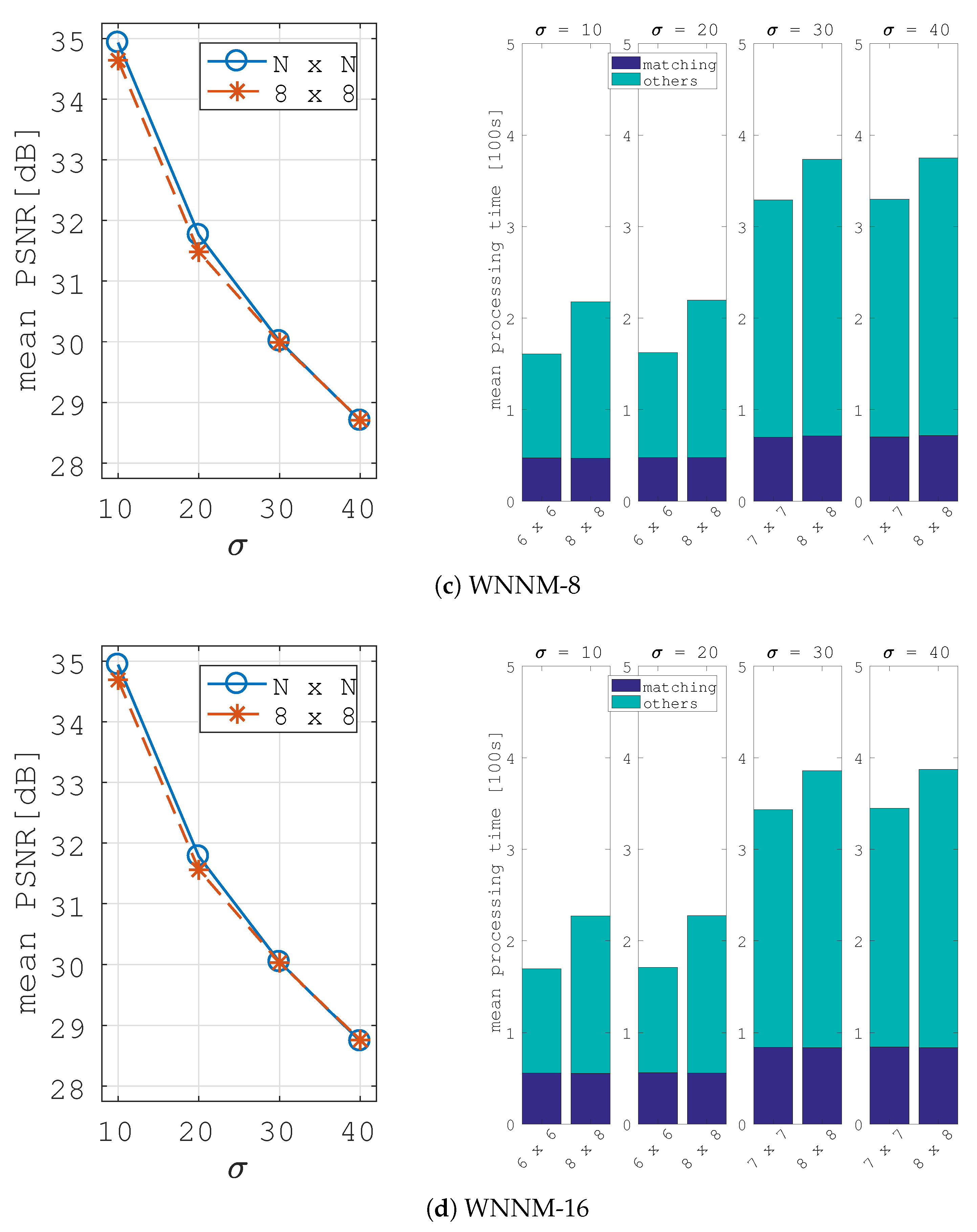
5. Image Denoising Application

We have compared the OTSHT to FS and the $8\times 8$ OHT [8] within the framework of image denoising, where the denoising performance depends on collecting similar patches. For this purpose, as an image denoising method, the weighted nuclear norm minimization (WNNM) [16] has been used. In WNNM, the optimal patch size and other parameters are set depending on noise level, which are shown in

Table 3. Parameters of WNNM.

$\mathbf{\sigma }$	N	Iteration	Similar Patches	Search Window
10	6	8	70	60 × 60
20	6	8	70	60 × 60
30	7	12	90	60 × 60
40	7	12	90	60 × 60
50	8	14	120	60 × 60

. Noise added to the image was white Gaussian with zero mean and the standard deviation of $\sigma$, where $\sigma =10,20,30,40$, and 50.

The OTSHT(OHT) and FS are used as the procedure of collecting similar patches in WNNM, which are referred to as WNNM-K and WNNM-FS, respectively. The pseudo code is shown in Algorithm 3. From the observation in Section 4.1 and Section 4.2, we constructed the OTSHT basis images from the balanced binary tree and used the non FS-equivalent algorithm where $K=2,4,8$, and 16 described in Section 3.2 because the speed up over FS cannot be expected when the patch size is small.

Algorithm 3: WNNM Image denoising.

Input: Noisy image y   1: Initialize ${\widehat{x}}^{\left(0\right)}=y$, $y^{\left(0\right)}=y$   2: for $i=1:ma{x}_i$   3:       Iterative regularization $y^{\left(i\right)}={\widehat{x}}^{(i-1)}+\delta (y-y^{(i-1)})$   4:       for each patch $y_t$ in $y^{\left(i\right)}$   5:             BM for collecting similar patches to form similar patch group ${\tilde{y}}_t$ by $SS{D}_j$   6:             estimate weight vector w   7:             singular value decomposition $[U,\Sigma ,V]=SVD\left({\tilde{y}}_t\right)$   8:             get the estimate: ${\widehat{x}}_t=U{S}_w(\Sigma )V^T$   9:       end 10:       aggregate ${\widehat{x}}_t$ to form the clean image ${\widehat{x}}^{\left(i\right)}$ 11: end Output: clean image ${\widehat{x}}^{\left(ma{x}_i\right)}$

First, we compare the OTSHT to FS. Figure 11a shows the mean PSNR of WNNM-FS and WNNM-K, $K=2,4,8,$ and 16 in different noise levels. The PSNR of WNNM-2 was below that of WNNM-FS but almost the same when the noise level is low. When $K\ge 4$, the PSNR of WNNM-K is almost the same as that of WNNM-FS. The PSNR of WNNM-16 is slightly higher than that of WNNM-FS. The PSNR of each image is shown in

Table 4. Mean PSNR of WNNM with FS (WNNM-FS) and WNNM with OTSHT and OHT using K limited basis images (WNNM-K) in different noise levels.

$\mathbf{\sigma }$= 10	WNNM-2		WNNM-4		WNNM-8		WNNM-16		WNNM-FS
	OTSHT	OHT	OTSHT	OHT	OTSHT	OHT	OTSHT	OHT
Lena	35.96	35.61	36.01	35.64	36.03	35.70	36.00	35.73	36.02
Barbara	35.13	34.80	35.31	34.95	35.35	35.03	35.47	35.12	35.49
boat	33.97	33.63	34.07	33.79	34.07	33.82	34.06	33.88	34.03
house	36.86	36.54	36.96	36.67	36.98	36.76	36.91	36.78	36.86
peppers	34.78	34.28	34.91	34.41	34.92	34.47	34.95	34.50	34.96
man	34.11	33.79	34.22	33.93	34.21	33.96	34.21	34.01	34.17
couple	33.98	33.66	34.11	33.79	34.10	33.83	34.12	33.88	34.11
hill	33.75	33.48	33.81	33.56	33.79	33.58	33.77	33.62	33.76
average	34.82	34.47	34.93	34.59	34.93	34.64	34.94	34.69	34.92
$\mathbf{\sigma }$= 20	WNNM-2		WNNM-4		WNNM-8		WNNM-16		WNNM-FS
	OTSHT	OHT	OTSHT	OHT	OTSHT	OHT	OTSHT	OHT
Lena	32.98	32.65	33.13	32.74	33.12	32.82	33.13	32.91	33.11
Barbara	31.71	31.44	31.94	31.62	32.00	31.76	32.14	31.89	32.15
boat	30.81	30.46	30.98	30.68	30.94	30.70	30.95	30.80	30.95
house	33.85	33.41	33.97	33.61	34.13	33.76	34.09	33.77	34.05
peppers	31.32	30.84	31.52	30.97	31.54	31.05	31.58	31.13	31.55
man	30.65	30.38	30.79	30.52	30.76	30.57	30.74	30.62	30.71
couple	30.59	30.30	30.83	30.52	30.79	30.56	30.81	30.63	30.77
hill	30.75	30.48	30.87	30.60	30.82	30.64	30.81	30.70	30.77
average	31.58	31.25	31.75	31.41	31.76	31.48	31.78	31.56	31.76
$\mathbf{\sigma }$= 30	WNNM-2		WNNM-4		WNNM-8		WNNM-16		WNNM-FS
	OTSHT	OHT	OTSHT	OHT	OTSHT	OHT	OTSHT	OHT
Lena	31.33	31.34	31.44	31.41	31.46	31.45	31.44	31.45	31.43
Barbara	29.90	29.96	30.11	30.14	30.17	30.22	30.27	30.32	30.28
boat	29.00	28.99	29.18	29.17	29.15	29.15	29.18	29.20	29.16
house	32.32	32.27	32.52	32.42	32.59	32.48	32.67	32.56	32.58
peppers	29.26	29.19	29.51	29.40	29.54	29.43	29.56	29.46	29.55
man	28.89	28.90	29.02	29.00	28.99	29.00	28.97	28.99	28.95
couple	28.72	28.73	28.94	28.94	28.96	28.96	28.97	28.99	28.94
hill	29.15	29.15	29.27	29.26	29.25	29.26	29.22	29.25	29.18
average	29.82	29.82	30.00	29.97	30.01	29.99	30.04	30.03	30.01
$\mathbf{\sigma }$= 40	WNNM-2		WNNM-4		WNNM-8		WNNM-16		WNNM-FS
	OTSHT	OHT	OTSHT	OHT	OTSHT	OHT	OTSHT	OHT
Lena	29.99	30.03	30.12	30.13	30.12	30.15	30.14	30.18	30.07
Barbara	28.44	28.55	28.63	28.71	28.68	28.79	28.74	28.87	28.75
boat	27.67	27.68	27.88	27.88	27.88	28.89	27.88	27.91	27.86
house	30.95	30.93	31.21	31.15	31.31	31.24	31.49	31.42	31.34
peppers	27.84	27.82	28.05	27.95	28.11	28.03	28.15	28.07	28.13
man	27.70	27.72	27.85	27.84	27.82	27.82	27.79	27.80	27.76
couple	27.38	27.43	27.58	27.60	27.63	27.66	27.63	27.69	27.58
hill	28.01	28.03	28.12	28.15	28.09	28.13	28.07	28.12	28.02
average	28.50	28.52	28.68	28.68	28.70	28.71	28.74	28.76	28.69
$\mathbf{\sigma }$= 50	WNNM-2		WNNM-4		WNNM-8		WNNM-16		WNNM-FS
	OTSHT	OHT	OTSHT	OHT	OTSHT	OHT	OTSHT	OHT
Lena	29.12		29.24		29.25		29.24		29.22
Barbara	27.52		27.72		27.75		27.81		27.82
boat	26.74		26.95		26.90		26.92		26.88
house	29.96		30.18		30.39		30.41		30.38
peppers	26.63		26.90		26.93		26.94		27.01
man	26.85		26.95		26.95		26.93		26.91
couple	26.47		26.62		26.62		26.64		26.63
hill	27.19		27.32		27.28		27.27		27.24
average	27.56		27.73		27.76		27.77		27.76

. The best PSNR is shown in bold. We observe that there is almost no difference of PSNR between WNNM-K and WNNM-FS, often the results of the first are even better, although FS is generally considered as more accurate than non-FS equivalent algorithm. The reason behind this is that BM in the spatial domain is not efficient for noisy images since it may result in matching noisy patterns, and thus, deceasing the denoising performance. The filtered images by these methods are almost undistinguishable. Figure 11b shows the mean processing time in different noise levels. The number of y-axis in the bar chart is the number of limited basis images, K. The processing time for BM and the other denoising method’s modules are expressed in blue and yellow bars, respectively. The processing time for BM of WNNM-2 is 46 to 56 percent of that of WNNM-FS; WNNM-4, 53 to 63%; and WNNM-8, 62 to 75%. In addition, the larger is the patch size, the more efficient is the procedure. The OTSHT reduces the processing time while keeping the same PSNR level as FS.

Next, we compare the OTSHT to the $8\times 8$ OHT used in WNNM-K ($K=2,4,8,$ and 16). Although the OHT cannot be used in WNNM with the optimal patch size, we force the $8\times 8$ OHT to WNNM by fixing the patch size to $8\times 8$ for evaluating the performance in the different patch sizes. Figure 12 shows the PSNR and processing time of the OTSHT and the $8\times 8$ OHT. The number of y-axis in the bar chart is the number of limited basis images, K, in the processing time. The processing time for BM and the other denoising method’s modules are expressed in blue and green bars, respectively. We observe the mean PSNRs of the OTSHT are larger than those of the $8\times 8$ OHT and the other processing time of the OTSHT is approximately 50 seconds faster than that of the $8\times 8$ OHT. This is due to the fact that the patches collected by the 8 × 8 OHT contain extra regions that are not appropriate for collecting similar patches and for processing in other modules. The PSNRs of each image are shown in Table 4, where the best PSNR is shown in bold. When $\sigma =10$ and 20, in WNNM-2 and WNNM-4, the PSNRs of OTSHT were 0.33 to 0.35 higher than those of OHT; WNNM-8, 0.28 to 0.29. When $\sigma >30$, the PSNRs of OTSHT were almost the same as those of OHT in WNNM-2, 4, 8, and 16.

6. Conclusions

We have considered the fast block matching (BM) based on orthonormal tree-structured Haar transform (OTSHT). We have described how to construct the two-dimensional OTSHT and use them for BM with a freedom of the design. The OTSHT can be used for FS-equivalent BM and non FS-equivalent one. In FS-equivalent BM, the conventional techniques, such as pruning and strip sum via integral image, are used for speed up. In non FS-equivalent BM, limited basis images are used. As a FS-equivalent BM, we have evaluated the computational complexity and pruning performance on the design of tree structures. We have demonstrated that the OTSHT based on balanced binary tree is more efficient than that based on the logarithmic binary tree, with respect to pruning performance and computational cost. As a non FS-equivalent BM, we have demonstrated the capability of the introduced method in image denoising application, where an arbitrary template size is used, depending on a noise level. In all our experiments, we have observed that not only PSNR values but also visual appearance of denoised images by WNNM-K and WNNM-FS are extremely close, so we can conclude that filtered images by these methods are almost indistinguishable. Thus, to conclude, the main advantage of the proposed WNNM-K is that it can effectively substitute a baseline WNNM (where FS is used for BM) providing a significant reduction of its computational time.

References

1. Dufour, R.; Miller, E.; Galatsanos, N. Template matching based object recognition with unknown geometric parameters. IEEE Trans. Image Process. 2002, 11, 1385–1396. [Google Scholar] [CrossRef] [PubMed] [Green Version]
2. Yuan, J.; Xu, D.; Xiong, H.-C.; Li, Z.-Y. A novel object tracking algorithm based on enhanced perception hash and online template matching. In Proceedings of the 2016 12th International Conference on Natural Computation, Fuzzy Systems and Knowledge Discovery (ICNC-FSKD), Changsha, China, 13–15 August 2016; pp. 494–499. [Google Scholar]
3. Ding, L.; Goshtasby, A.; Satter, M. Volume image registration by template matching. Image Vis. Comput. 2001, 19, 821–832. [Google Scholar] [CrossRef]
4. Sarraf, S.; Saverino, C.; Colestani, A.M. A robust and adaptive decision-making algorithm for detecting brain networks using functional mri within the spatial and frequency domain. In Proceedings of the 2016 IEEE-EMBS International Conference on Biomedical and Health Informatics (BHI), Las Vegas, NV, USA, 24–27 February 2016; pp. 53–56. [Google Scholar]
5. Sarraf, S.; Anderson, J.; Tofighi, G. Deepad: Alzheimer disease classification via deep convolutional neural networks using MRI and fMRI. bioRxiv 2016, 070441. [Google Scholar] [CrossRef]
6. Ouyang, W.; Tombari, F.; Mattocia, S.; Stefano, L.D.; Cham, W.-K. Performance Evaluation of Full Search Equivalent Pattern Matching Algorithms. IEEE Trans. Pattern Anal. Mach. Intell. 2012, 34, 127–143. [Google Scholar] [CrossRef] [PubMed]
7. Tombari, F.; Mattoccia, S.; Stefano, L.D. Full search-equivalent pattern matching with incremental dissimilarity approximations. IEEE Trans. Pattern Anal. Mach. Intell. 2009, 31, 129–141. [Google Scholar] [CrossRef] [PubMed]
8. Ouyang, W.; Zhang, R.; Cham, W.-K. Fast pattern matching using orthogonal Haar transform. In Proceedings of the 2010 IEEE Computer Society Conference on Computer Vision and Pattern Recognition, San Francisco, CA, USA, 13–18 June 2010; pp. 3050–3057. [Google Scholar]
9. Ouyang, W.; Cham, W.K. Fast algorithm for Walsh Hadamard transform on sliding windows. IEEE Trans. Pattern Anal. Mach. Intell. 2010, 32, 165–171. [Google Scholar] [CrossRef] [PubMed]
10. Moshe, Y.; Hel-Or, H. Video block motion estimation based on Gray-code kernels. IEEE Trans. Image Process. 2009, 18, 2243–2254. [Google Scholar] [CrossRef] [PubMed]
11. Crow, F. Summed-area tables for texture mapping. ACM SIGGRAPH Comput. Graph. 1984, 18, 207–212. [Google Scholar] [CrossRef]
12. Viola, P.; Jones, M.J. Robust real-time object detection. Int. J. Comput. Vis. 2001, 57, 37–154. [Google Scholar]
13. Li, Y.; Li, H.; Cai, Z. Fast orthogonal Haar transform pattern matching via image square sum. IEEE Trans. Pattern Anal. Mach. Intell. 2014, 36, 1748–1760. [Google Scholar] [CrossRef] [PubMed]
14. Alkhansari, M.G. A fast globally optimal algorithm for template matching using low-resolution pruning. IEEE Trans. Image Process. 2001, 10, 526–533. [Google Scholar] [CrossRef] [PubMed]
15. Buades, A.; Coll, B.; Morel, J.-M. A non-local algorithm for image denoising. In Proceedings of the 2005 IEEE Computer Society Conference on Computer Vision and Pattern Recognition (CVPR’05), San Diego, CA, USA, 20–25 June 2005; pp. 60–65. [Google Scholar]
16. Gu, S.; Zhang, L.; Zuo, W.; Feng, X. Weighted nuclear norm minimization with application to image denoising. In Proceedings of the 2014 IEEE Conference on Computer Vision and Pattern Recognition, Columbus, OH, USA, 23–28 June 2014; pp. 2862–2869. [Google Scholar]
17. Dabov, K.; Foi, A.; Katkovnik, V.; Egiazarian, K. Image denoising by 3D transform-domain collaborative filtering. IEEE Trans. Image Process. 2007, 16, 2080–2095. [Google Scholar] [CrossRef] [PubMed]
18. Criminisi, A.; Perez, P.; Toyama, K. Region Filling and Object Removal by Exemplar-Based Image Inpainting. IEEE Trans. Image Process. 2004, 13, 1200–1212. [Google Scholar] [CrossRef] [PubMed] [Green Version]
19. Wexler, Y.; Shechtman, E.; Irani, M. Space-Time Completion of Video. IEEE Trans. Pattern Anal. Mach. Intell. 2007, 29, 463–476. [Google Scholar] [CrossRef] [PubMed] [Green Version]
20. Egiazarian, K.; Astola, J. Tree-structured Haar Transform. J. Math. Imaging Vis. 2002, 16, 269–279. [Google Scholar] [CrossRef]
21. Ito, I.; Egiazarian, K. Design of orthonormal Haar-like features for fast pattern matching. In Proceedings of the 2017 25th European Signal Processing Conference (EUSIPCO), Kos, Greece, 28 August–2 September 2017; pp. 2452–2456. [Google Scholar]
22. Ito, I.; Egiazarian, K. Full search equivalent fast block matching using orthonormal tree-structured Haar transform. In Proceedings of the 10th International Symposium on Image and Signal Processing and Analysis), Ljubljana, Slovenia, 18–20 September 2017. [Google Scholar] [CrossRef]
23. Image Denoising with Block-Matching and 3D Filtering. Available online: http://www.cs.tut.fi/~foi/3D-DFT/ (accessed on 14 September 2018).
Figure 1. Binary tree and its interval.
Jimaging 04 00131 g001
Figure 2. Decomposition of space I α × I β . First, the region is divided by φ i . Next, the positive region in white is divided by φ 2 , Finally, the negative region in black is divided by φ 3 . This procedure is iterated until all space cannot be divided.
Jimaging 04 00131 g002
Figure 3. Appearance of constructing the basis images of size 3 × 3 .
Jimaging 04 00131 g003
Figure 4. An example of OTSHT basis images based on a balanced binary tree having five leaves.
Jimaging 04 00131 g004
Figure 5. An example of OTSHT basis images based on a logarithmic binary tree having five leaves.
Jimaging 04 00131 g005
Figure 6. An example of OHT basis images based on a full binary tree having four leaves.
Jimaging 04 00131 g006
Figure 7. The number of operations per pixel for computing B-OTSHT and L-OTSHT coefficients using strip sum (S) and integral image only (I).
Jimaging 04 00131 g007
Figure 8. Five examples of binary tree having nine leaves.
Jimaging 04 00131 g008
Figure 9. Percentage of remaining windows after pruning that is conducted every k-th basis images.
Jimaging 04 00131 g009
Figure 10. Mean processing time of OTSHT vs. FS. 100 templates are used for evaluation.
Jimaging 04 00131 g010
Figure 11. OTSHT vs. FS. (a) Mean PSNR and (b) mean processing time of WNNM-FS and WNNM-K in different noise levels. In the bar chart, the number and ‘F’ of y-axis are the number of limited basis images and FS, respectively.
Jimaging 04 00131 g011
Figure 12. OTSHT vs. the 8 × 8 OHT. Mean PSNR and mean processing time of WNNM-K in different noise levels. In the chart, 8 × 8 denotes OHT; otherwise, OTSHT.
Jimaging 04 00131 g012aJimaging 04 00131 g012b