Image-Based Surrogates of Socio-Economic Status in Urban Neighborhoods Using Deep Multiple Instance Learning

Abstract

(1) Background: Evidence-based policymaking requires data about the local population’s socioeconomic status (SES) at detailed geographical level, however, such information is often not available, or is too expensive to acquire. Researchers have proposed solutions to estimate SES indicators by analyzing Google Street View images, however, these methods are also resource-intensive, since they require large volumes of manually labeled training data. (2) Methods: We propose a methodology for automatically computing surrogate variables of SES indicators using street images of parked cars and deep multiple instance learning. Our approach does not require any manually created labels, apart from data already available by statistical authorities, while the entire pipeline for image acquisition, parked car detection, car classification, and surrogate variable computation is fully automated. The proposed surrogate variables are then used in linear regression models to estimate the target SES indicators. (3) Results: We implement and evaluate a model based on the proposed surrogate variable at 30 municipalities of varying SES in Greece. Our model has $R^2=0.76$ and a correlation coefficient of $0.874$ with the true unemployment rate, while it achieves a mean absolute percentage error of $0.089$ and mean absolute error of $1.87$ on a held-out test set. Similar results are also obtained for other socioeconomic indicators, related to education level and occupational prestige. (4) Conclusions: The proposed methodology can be used to estimate SES indicators at the local level automatically, using images of parked cars detected via Google Street View, without the need for any manual labeling effort.

1. Introduction

For the past 30 years, there has been a growing need for Evidence-Based Policymaking (EBP), led by the desire to transition from decisions based on expertise and authority, to decisions supported and evaluated by data and scientific findings [1]. EBP has been actively promoted by the UK Government since 1997, starting with the famous “Modernising Government” white paper [2], while the USA is also seeking to better integrate data and other forms of evidence to federal EBP processes, as can be seen by the establishment and findings of the Commission on Evidence-Based Policymaking [3].

Acquiring evidence to support EBP, however, is far from straightforward. Research and data analysis requires money and time, and sufficient evidence may not be available for policy formulation when decisions are being made [4]. Furthermore, even when research evidence exists, it may not apply locally, which calls for even further investigation at the local context to support targeted policies [5], introducing additional costs, possibly beyond cost-effectiveness thresholds. Sub-optimal, “blanket” policies at the macroscopic level are applied instead [6].

Local measurements and demographics are therefore key to EBP, with the main sources of such information currently being census data, which will probably be combined with additional data from government agencies in the future [3]. Census data collection is expensive, however, with the 2010 USA decennial census costing over $13 billion [7], while the collected information is limited and may quickly become outdated, given that a general census is performed every 10 years.

Although these problems pose significant challenges to EBP, recent technical achievements are now offering innovative means of obtaining objective measurements of the social and urban environment. Services such as Google Street View (GSV) [8,9], Bing Maps Streetside [10], and OpenStreetCam [11] are now offering geo-located urban images and allow researchers to virtually explore the environment and measure its characteristics. For instance, researchers of the SPOTLIGHT project [12] developed a GSV-based “virtual audit” tool [13] to help reduce the effort required to quantify the typology of different neighborhoods in European cities. They then used the images of each local neighborhood to objectively measure urban features associated with obesity [14].

Moving beyond virtual audits, Gebru et al. [15] used GSV images and deep learning to automatically detect the distribution of different car models in each neighborhood (including car make, model, and year). Analysis of 50 million images from 200 US cities showed that such data can be used to automatically infer local demographic information related to income, education, race, and voter preferences. Most notably, this information was estimated at the US precinct level (each including approximately 1000 people). Development of the car classifiers used in that work was, however, a challenging task in itself. It involved 2657 car categories and almost 400,000 images which were manually annotated to indicate the category of all visible cars in each image. Annotators through Amazon Mechanical Turk as well as car experts were recruited to carry out this laborious task.

In our work in the BigO project [16], we aim to identify local factors of the urban and socioeconomic environment that are linked to obesogenic behaviors of children, such as low physical activity and unhealthy eating habits. This information can then be used to design targeted interventions and policies that take into account the local context. Motivated by our need for SES indicators of the local urban population, we explore whether the approach of Gebru et al. [15] can be used to infer such information from cars, but without the associated manual annotation effort.

To achieve this, we approach the car categorization problem using models trained with multiple instance learning at municipality level. Specifically, instead of annotating cars, we annotate municipalities based on their socio-economic status. We then train a deep learning model to categorize car images based on the type of municipality that they were observed in. Finally, we produce an aggregate score based on the model output for approximately 500 cars sampled from each municipality via GSV. Results from 30 municipalities of varying SES in Greece indicate that this method can accurately predict indicators of socio-economic status, such as the local unemployment rate. Specifically, a linear regression model trained on 25 municipalities (8 low, 9 average, and 8 high SES) achieves a coefficient of determination of $R^2=0.76$ while evaluation on a held-out test set of 5 additional municipalities (also of varying SES) reaches a mean absolute percentage error of $0.089$ and mean absolute error of $1.87$. Other SES indicators, related to education level and occupational prestige are evaluated as well, leading to linear regression models with similar effectiveness.

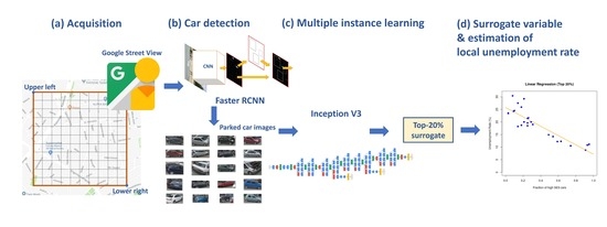
These results show that we can leverage deep learning object recognition models and multiple instance learning to produce surrogates of local socio-economic indicators at a minimal cost. An illustration summarizing the main steps of the proposed method is shown in Figure 1. These are discussed in detail in the following Sections.

The rest of the paper is organized as follows. Section 2 summarizes relevant work in the field of using visual analysis to measure environment characteristics and to estimate demographics, SES indicators, or perceptions of the local population about their environment. Section 3 presents our method for image-based neighborhood characterization using deep multiple instance learning, while Section 4 presents the results of experimental evaluation in Greek municipalities. Finally, Section 5 summarizes our findings and concludes this work.

2. Related Work

Google Street View has been extensively used to measure characteristics of the built environment and to infer demographics. Originally, researchers suggested to use Street View to perform virtual auditing in order to avoid the cost and time required for field audits. In Reference [19], a comparison between a 2007 field audit and 2008 virtual audit for 143 variables in a part of New York showed high agreement (over 80%) for more than half of the variables. Agreement was lower for items that typically exhibit temporal variability (e.g., variables related to the presence of people, animals, or garbage and litter). Similar results were reported in Reference [20], concluding that GSV provides a resource-efficient and reliable alternative to fields audits for attributes associated to walking and cycling.

Similar tools have also been developed to discover associations between characteristics of the built environment and obesity. Researchers that developed the SPOTLIGHT virtual audit tool to assess obesogenic characteristics of the built environment [12,13,14] used both field and virtual audits. They reported very high intra-observer (96.4%) and inter-observer (91.5%) agreement for multiple environmental characteristics in four Dutch neighborhoods. Recently, Bader et al. [21] concluded that GSV for virtual auditing is reliable, but researchers need to carefully consider issues related to selection of variables (as also originally discussed in Reference [19]), as well as rater fatigue, which can be a significant source of error.

To mitigate the errors, effort, and cost of manual measurements, several researchers have resorted to computer vision and machine learning algorithms to automate measurement tasks. Perhaps the most well-known example is by Google itself, where Goodfellow et al. [22] used GSV images to automatically record street numbers of houses for use in the Google Maps service [23]. A deep Convolutional Neural Network (CNN) was used for simultaneously performing number localization, segmentation, and recognition. The large number of available training images (tens of millions of images) allowed the system to reach very high effectiveness (over 96% overall), despite the large number of model parameters.

There have also been several subsequent efforts towards automatic measurement of features of the environment or points of interest through GSV images. In Reference [24] the authors present an urban object cataloging system, which can accurately localize and classify trees detected in urban neighborhoods through GSV. In Reference [25,26,27] different methods are presented for storefront detection and classification from street-level images.

All these works aim at measuring environment variables which are directly visible through GSV images. Another body of work aims at using GSV images to capture measurements which can be inferred through characteristics of the environment. For example, in Reference [28] the authors use the Place Pulse dataset [29] to build a deep learning model of safety perception from GSV images and correlate this with the liveliness of neighborhoods, as measured from mobile phone data. In Reference [30] the authors use GSV images to determine the number of pedestrians present in street segments in order to estimate pedestrian volume, while in Reference [31] the authors automatically extract three measures of visual enclosure which are shown to be correlated with walkability. Moving even further, Reference [32] uses features of the built environment, extracted through CNN and builds regression models that associate these features with adult obesity prevalence.

In this paper we start from the approach of Gebru and others [15,33] (see Section 1) and explore whether it is possible to develop classification models to infer socioeconomic indicators without the need for any manual annotations. To achieve this, we propose to build car classification models based on the differences in car visual appearance between low and high SES areas using multiple instance learning. We introduce a score that acts as a surrogate of the local SES and use it with simple linear regression to build models that predict the local unemployment rate and other SES indicators, with highly encouraging results.

3. Multiple Instance Learning for Neighborhood Characterization Using Images

3.1. Data Acquisition

The first step of our method involves the collection of GSV side-view images of parked cars in the region of interest. In this work, we use rectangular regions, defined by two sets of coordinates indicating the upper left and lower right points of the rectangle (see Figure 1, Step (a)). To ensure that only data from the administrative regions of interest are selected during sampling, we ignore any points of the grid that fall outside the administrative region boundaries, as defined by GIS data.

The region is first traversed to acquire the candidate images. Specifically, we select points on a dense, regular rectangular grid inside the region of interest, with a fixed distance step in each direction. To obtain the point coordinates we need to consider the earth’s curvature. For the area sizes we are interested in, we can assume that earth is a perfect sphere and we can rely on the haversine formula that provides the distance between two points,

$$d(p_1,p_2)=2\rho \arcsin \left(\sqrt{{\sin }^2\left(\frac{{\varphi }_2-{\varphi }_1}{2}\right)+\cos ({\varphi }_1)\cos ({\varphi }_2){\sin }^2\left(\frac{{\lambda }_2-{\lambda }_1}{2}\right)}\right)$$

(1)

where $\rho =6371\times {10}^3$ is the earth’s radius in meters and ${\varphi }_i,{\lambda }_i$, are the point $p_i$, coordinates (latitude and longitude, respectively) in radians, with $i=1,2$. This formula allows us to convert the desired sampling step in meters to a step in radians along the latitude and longitude directions. If $d_A$ and $d_B$ are the lengths of the sides of the rectangle in the latitude and longitude direction, respectively (determined through Equation (1)), and $s_A$, $s_B$ are the corresponding steps in meters, then $n_A=d_A/s_A$ and $n_B=d_B/s_B$ are the number of grid points in each direction. The steps, in radians, are then $r_A=d_A/n_A$ and $r_B=d_B/n_B$. Note that if a grid point falls out of the boundaries of the administrative region of interest, it is rejected.

We query the GSV Application Programming Interface (API) [9], provided by Google, for metadata regarding each point in the rectangular grid. The API does not provide data about the query point; instead, it provides metadata for the closest location with a street image available (without returning the image itself). This allows us to determine a set of unique locations with available images that are close to the selected rectangular grid points. If the sampling step becomes small enough, we obtain the list of all available locations with GSV street images.

In this work, we focus on parked cars, to minimize the effect of cars passing through a neighborhood on the extracted measurements. This also reduces the variability of the visual appearance of cars, which may have an impact on the classification model used in later stages. It is worth mentioning, however, that we performed our experiments in Greece, where cars are commonly parked on the street in urban regions. In other parts of the world, where garages or parking lots are more common, it is worth including moving cars also, to avoid introducing bias in the sampling procedure.

Acquisition of parked cars requires that for each location with street images, we need to obtain two pictures that are vertical (left and right) to the street direction at the selected point and detect parked cars. The street heading at that point is determined through Google’s geocoding API [34] by querying a neighboring point on the same street. More specifically, for each location, we obtain the location of either the previous or the next street number using the geocoding API. The bearing formula is used to determine the street heading

$$\theta =\mathrm{atan}2\left(\sin \right(\Delta \lambda )\cos \left({\varphi }_2\right),\cos \left({\varphi }_1\right)\sin \left({\varphi }_2\right)-\sin \left({\varphi }_1\right)\cos \left({\varphi }_2\right)\cos (\Delta \lambda \left)\right)$$

(2)

where $\Delta \lambda$ is the difference in longitude between the two points and ${\varphi }_1$, ${\varphi }_2$ the point latitudes. We can then obtain street side views by querying GSV for headings $\pm {90}^{°}$ from the street heading at the selected point. This process is repeated for all selected locations in the region. We then process the images to detect cars.

3.2. Car Detection with Faster R-CNN

To detect cars in the retrieved side-view images (Step (b) in Figure 1), we use a Faster R-CNN [17] model pre-trained on Pascal VOC 2007 [35]. Faster R-CNN is a popular object detection deep neural network architecture, which extends Fast R-CNN [36] with the addition of a trainable Region Proposal Network for producing candidate object regions in the input image. The model that we used in our experiments initially processes the data using the first 13 convolutional layers of VGG-16 [37], pre-trained on ImageNet. The output of the convolutional layers, C, is processed by a Region Proposal Network (RPN) which includes a regression layer, providing candidate object region boundaries, and a classification layer which identifies image regions as “object” or “non-object”. The same output, C, is passed on to the Fast R-CNN RoI pooling layer for the candidate object regions detected by the RPN. The RoI pooling layer performs max pooling to convert the object region proposal to a fixed-size representation. A final classification step determines the detected object class. For additional details on Faster R-CNN the reader is referred to Reference [17].

In this work, we applied Faster R-CNN for the “Car” object class only. By applying Faster R-CNN to the images collected from GSV (Section 3.1) with a 0.8 detection threshold, we obtained a collection of parked car images from the target region with almost no false positives. As described in the following sections, the missed detections do not affect the proposed methodology, since it uses only a sample of the cars in each region and therefore high recall is not necessary.

3.3. Automatic Labeling of Cars Using Multiple Instance Learning

Motivated by the results of Reference [15], we develop our models based on the premise that the types of cars observed in an urban region are indicators of the socio-economic status of the local population. Instead of attempting to detect the exact category (i.e., make, model, and year) of each car, however, we simplify the learning task as much as possible and try to build a binary classification model using multiple instance learning [38], without any manual car labels.

More specifically, we label regions as “low” and “high” SES based on published SES indicators. In the experiments of this paper we applied our method to Greek municipalities and relied on the local unemployment rate to assign a label at municipality level. Every car detected in a selected municipality (following the process described in Section 3.2) is also labeled as “low” and “high” depending on the municipality’s label. In other words, the characterization of each detected car image depends on the region it was observed in, rather than the car category. This has several implications:

• All cars observed in a single urban region (e.g., same postal code or municipality) inherit the same label during training.
• It is possible that different instances of the same car category are annotated as both “low” and “high” during model training.
• The model is built based on the overall car appearance and a classifier may learn distinguishing characteristics besides the car category, such as the car’s age, and overall exterior state.

The use of multiple instance learning eliminates the labeling effort for training our classifier models, and may also help our models identify distinguishing characteristics of the visual appearance of cars between low and high SES regions. On the other hand, it significantly increases the level of training noise. To minimize the impact of noise, while maintaining the benefits of multiple instance learning, we propose to train the classifier model using regions at the low and high SES extremes, based on available statistical authority data. This has the potential to help the training procedure, by amplifying the differences in car types and car appearances between the high and low SES regions. Furthermore, as we will discuss in the next section, we rely only on the car instances classified with high confidence (probability close to 1 or 0) by our model to minimize the effect of noise in estimating the region’s SES indicators.

The binary classifier used in this work was built based on an Inception V3 model [18], pre-trained on ImageNet, as provided by the Tensorflow deep learning framework [39]. Only the last fully connected layer of the Inception model was re-trained to classify cars as originating from low or high SES regions. During training, each detected car image was cropped and resized to $224\times 224$ pixels and was transformed using standard random input distortions to improve model generalization. The result of training is a model that receives a cropped car image (the resized output of the Faster R-CNN model) and computes the probability that the input car image originates from a high SES region.

3.4. Image-Based Surrogates of Socioeconomic Status

Using the images of parked cars from GSV and the output of the deep multiple instance learning model of Section 3.3, we can compute quantities which can act as surrogates of SES indicators of the local population. In this paper, we focus on local unemployment rate as the representative SES indicator and attempt to predict it using simple linear regression over the surrogate variable, i.e., $\widehat{y}=w_{1}x+w_0$, where $\widehat{y}$ is the estimate of the local unemployment rate, y, and x is the surrogate variable.

We propose to set x equal to the fraction of cars classified as originating from a high SES region, for those images with the highest classification confidence (either positive or negative). Specifically, given the output $p\left(high\right|I)$ of the model for each car image I detected at the local neighborhood or municipality, we compute the fraction only for the cars classified with the top 20% confidence

$$c\left(I\right)=\{\begin{array}{cc}p\left(high\right|I)\hfill & \mathrm{if}p\left(high\right|I)>0.5\hfill \\ 1-p\left(high\right|I)\hfill & \mathrm{if}p\left(high\right|I)\le 0.5\hfill \end{array}$$

(3)

Then

$$x=\frac{|\{I|p(high\left|I\right)>0.5,c\left(I\right)\in \mathrm{top}-20\%\}|}{|\{I|c(I)\in \mathrm{top}-20\%\}|}$$

(4)

where “top-20%” indicates the top 20% classification confidence scores, c (or, equivalently, the c values above the 80th percentile) and the symbol $|.|$ denotes set cardinality.

This choice mitigates, to a degree, the problem of noise introduced by multiple instance learning. A probability $p\left(high\right|I)$ close to 0 or 1 indicates high confidence about the label of I. On the other hand, a probability close to 0.5 indicates complete uncertainty over the car’s class, i.e., a car that could be observed in high or low SES regions with equal probability. By considering cars with the top-20% classification confidence, we ensure that we select cars that are most discriminative between low and high SES regions. This approach also highlights the differences between high and low SES regions, which would otherwise be less apparent with a large number of average-scoring cars.

4. Experiments

We performed experiments using GSV images retrieved from 30 municipalities in Greece. The experiments aim at demonstrating the effectiveness of the car classification models, as well as of the SES indicator prediction models, despite the noise introduced by multiple instance learning. Furthermore, we show how the proposed approach can be used to estimate local SES indicators at high geographical resolution.

Since average income information is not available for Greece at detailed geographical level, we used unemployment rate as the local SES indicator, as provided by the Hellenic Statistical Authority [40]. Use of additional indicators related to education level and occupational prestige is also explored. We followed the approach described in Section 3.1 for image acquisition and we chose the appropriate grid step (and number of images) to detect approximately 500 cars within each municipality, using Faster R-CNN. We consider this to be a representative sample of the cars in each municipality.

4.1. Assessing the Accuracy of the Multiple Instance Learning Models

We initially performed a small-scale evaluation of the pre-trained, state of the art car detection model (Section 3.2), on a set of 1000 urban GSV images, randomly selected using our data acquisition method (Section 3.1). Out of a total of 350 parked cars contained in these images, Faster R-CNN with 0.8 threshold detected 238 cars, 1 false detection, as well as 12 moving cars, that were mistakenly considered as parked cars. This indicates approximately 70% parked car detection accuracy, and 5% misclassification error due to moving cars wrongly assumed to be parked cars. Our approach therefore detects parked cars with very high accuracy. As for the missed car detections, these do not affect our method since it is based on a sampling of the region’s cars.

Given the list of all municipalities in Greece, we first selected the five with the highest and the five with the lowest unemployment rate to assess the accuracy of the car classification model. The differences between municipalities are significant, with the highest SES municipality (Psychiko, in the Athens region) having 8.8% unemployment rate and the lowest SES municipality (Ampelokipoi/Menemeni, in the Thessaloniki region) 30.4%. Each car detected with Faster R-CNN in the top 5 municipalities (Section 3.2) is assigned the “high” SES label, while cars in the bottom 5 municipalities are assigned the “low” SES label. We then used multiple instance learning to train and evaluate the car classification model based on Inception V3, as described in Section 3.3.

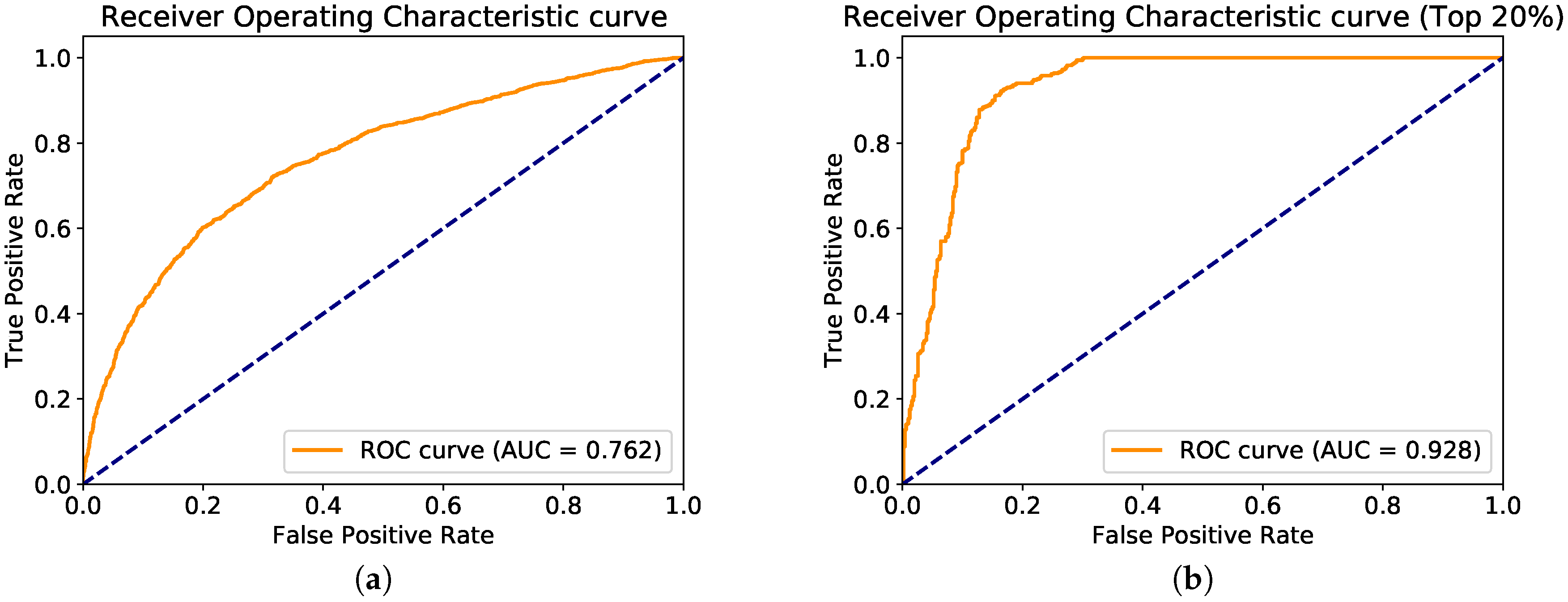
Evaluation of the car classifiers was initially performed on these 10 municipalities only, using a Leave-One-Group-Out (LOGO) approach. LOGO is a variant of the Leave-One-Out (LOO) test error estimation, where a group of samples is left out for each evaluation iteration. In our case, each group corresponds to the cars of a single municipality. Specifically, ten evaluation iterations are performed. During each iteration, car images from one municipality are left out and the last fully connected layer of the Inception V3 model is re-trained on the images of the remaining municipalities. The resulting model is then used to classify each car of the left-out municipality. For each car, we wish to predict the label of the originating municipality. This is not always possible, since the same type of car may be present in both low and high SES municipalities. Still, we can use this evaluation approach to examine if any differences are detected by our model between the regions of varying SES. The resulting confusion matrix is shown in a of

Table 1. Confusion matrices of the car classification models.

(a) Results for All Cars of Each Municipality
		Predicted (All)
		High	Low
Actual	high	1660	714
	low	739	1713
Accuracy: 0.699
(b) Results for the Cars With Highest Confidence
		Predicted (Top 20%)
		High	Low
Actual	high	412	88
	low	71	429
Accuracy: 0.841

. In addition, Figure 2a shows the model’s Receiver Operating Characteristic (ROC) curve. Our model achieves an accuracy of 0.699 and area under the curve (AUC) of 0.762.

These results are significantly better than random selection, indicating that the models identify differences between low and high SES regions. As discussed in Section 3.4, however, we can further amplify the differences between low and high SES municipalities by evaluating only the cars with top 20% classification confidence (3). In our case, this corresponds to the 100 most confident predictions (since we sample 500 cars per municipality). Results are shown in b of Table 1 and Figure 2b, where we can see that for the top-20% cars of each region the prediction of the originating municipality SES is much more accurate. In this case, our model achieves 0.841 accuracy and 0.928 AUC. One could also select images using absolute confidence thresholds, although we chose to use the top-20% method to ensure that the same, sufficient number of samples was used to compute the surrogate score for all municipalities.

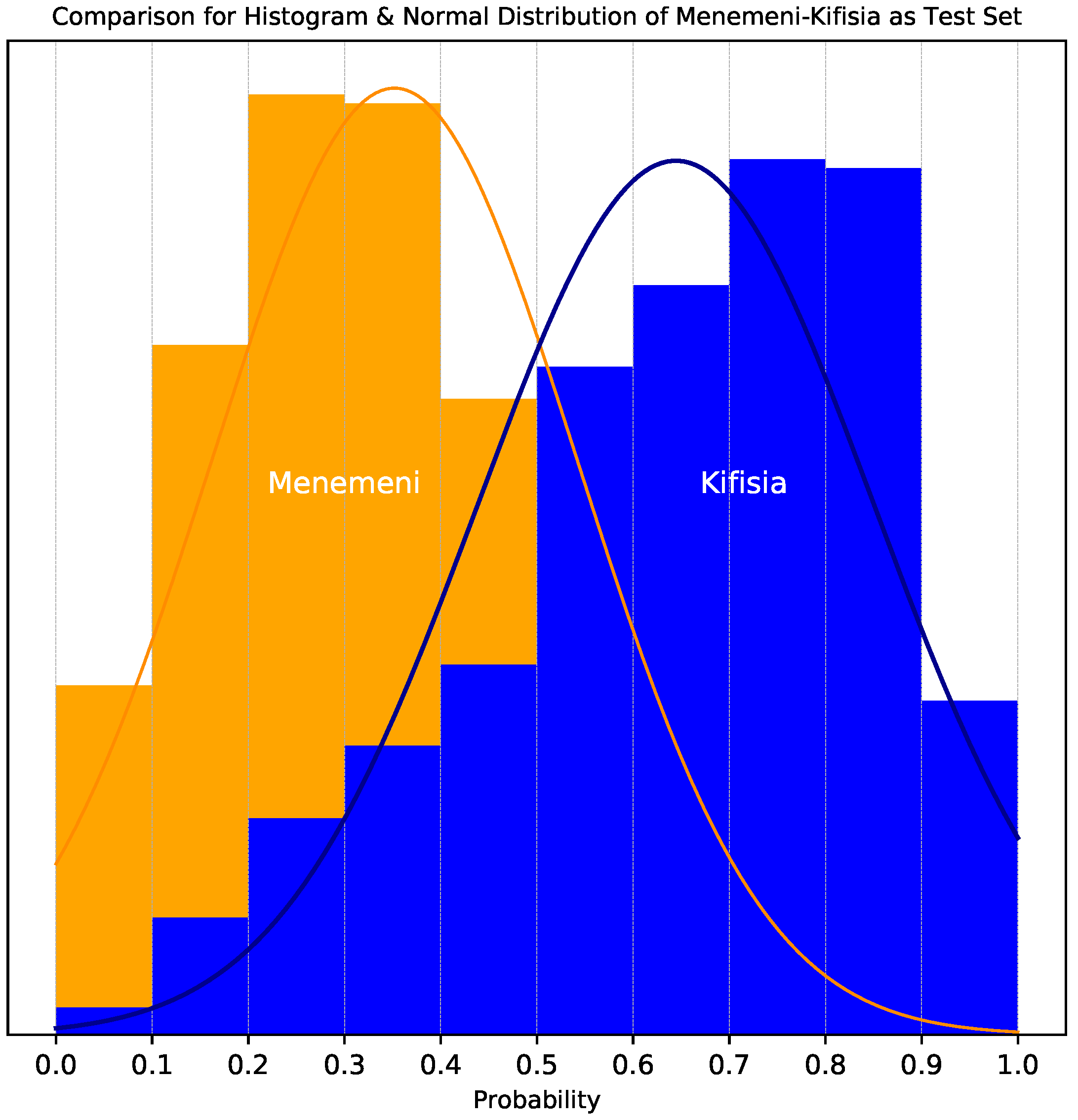
To further support the argument for using the top-20% predictions, Figure 3 illustrates the distribution of all scores provided by our model for the cars in a high SES municipality (Kifisia, in Athens) and a low SES municipality (Ampelokipoi/Menemeni, in Thessaloniki). We observe that for the high SES region, the mean of the classifier scores is 0.35, while for the low SES region it is 0.65. Furthermore, the high SES region has a significantly higher percentage of cars with score close to 1, while the low SES region has more cars with scores close to 0.

These observations hint to the definition of the surrogate indicator defined in Equation (4), i.e., the percentage of cars classified as high SES in the top-20% confidence cars. The surrogate indicator will be evaluated next.

4.2. Estimating the Unemployment Rate of Greek Cities

The models that we evaluated in Section 4.1 were built using the five highest and five lowest unemployment rate Greek municipalities. In this Section, we use the car classification model trained on these municipalities to compute the image-based surrogate and the local unemployment rate for other municipalities in Greece.

First, we select an additional 15 Greek municipalities, including 3 low unemployment rate, 3 high unemployment rate, and 9 close to the median unemployment rate (which, for Greece, is approximately 20%). The list of 25 municipalities selected so far, as well as their unemployment rate, is shown in

Table 2. The 25 municipalities used to create our linear model, as well as their unemployment rate (y), surrogate score (x), model prediction ($\widehat{y}$), and absolute error. Municipalities are grouped into high-medium-low unemployment rate, based on statistical authority data. The average cars per Google Street View (GSV) image is also shown (which, in this case, is not highly correlated with unemployment rate).

Municipality	y (%)	x	$\widehat{\mathit{y}}(\%)$	$|\mathit{y}-\widehat{\mathit{y}}|(\%)$	Avg. Cars/Image
Amp./Menemeni	30.4	0.08	24.26	6.14	1.306
Aspropyrgos	29.2	0.21	21.84	7.36	0.401
P. Mela	27.5	0.14	23.15	4.35	0.884
Perama	25.9	0.18	22.40	3.5	0.655
Evosmos	24.5	0.1	23.89	0.61	1.258
Fylis	24.2	0.09	24.06	0.14	0.227
Agrinio	23.5	0.03	25.19	1.69	0.804
Salamina	23.4	0.03	25.19	1.79	0.409
Patra	21.6	0.26	20.91	0.69	0.586
Kavala	21.4	0.25	21.10	0.3	0.489
Volos	20.0	0.29	20.35	0.35	0.62
Serres	20.0	0.21	21.84	1.84	1.039
Lamia	19.6	0.25	21.10	1.5	0.65
Heraklion	19.0	0.31	19.98	0.98	0.898
Komotini	18.7	0.18	22.40	3.7	0.675
Larissa	18.5	0.25	21.10	2.6	0.492
Edessa	18.2	0.14	23.15	4.95	0.679
Pylaia-Chortiatis	14.9	0.49	16.63	1.73	0.665
Glyfada	14.2	0.54	15.70	1.5	0.924
Marousi	12.3	0.63	14.03	1.73	0.785
Voula	12.2	0.59	14.77	2.57	0.371
Dionysos	11.1	0.95	8.075	3.02	0.198
Kifisia	10.8	0.93	8.45	2.35	0.605
Vrilissia	10.5	0.74	11.98	1.48	0.447
Psychiko	8.8	0.91	8.82	0.02	0.462

(the other columns of the table will be discussed in the following). For each municipality, we apply the car classification model and compute the image-based surrogate of Equation (4).

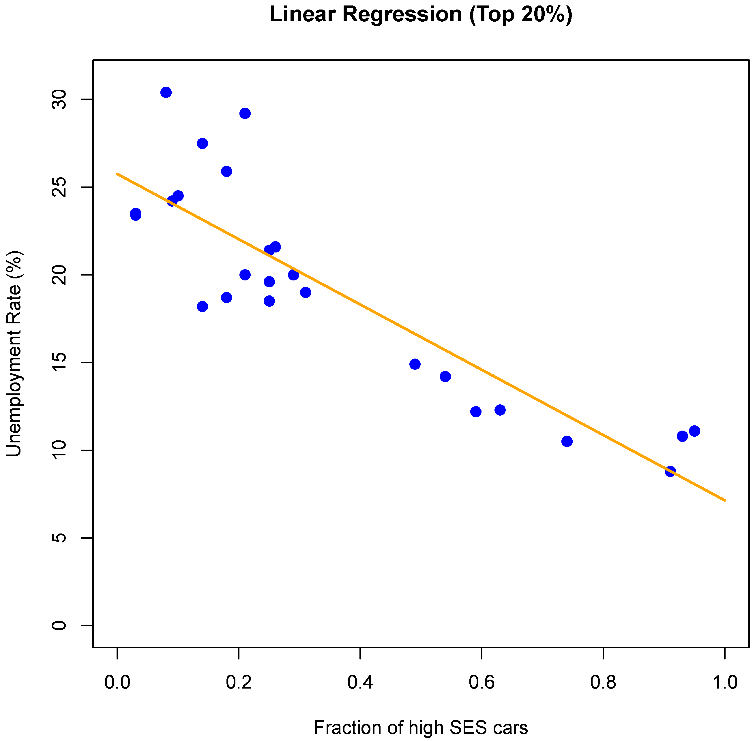
We build a linear model, $\widehat{y}=w_{1}x+w_0$, to predict the unemployment rate y using the surrogate x. The resulting model is

$$\widehat{y}=-18.6062x+25.7505$$

(5)

where x is the surrogate variable and $\widehat{y}$ is the unemployment rate estimate. A visual representation of the model’s prediction vs. the actual unemployment rate is shown in Figure 4.

The statistical analysis of the model is shown in

Table 3. Analysis of the linear regression model of the proposed surrogate variable.

Residuals:
	Min	1Q	Median	3Q	Max
	$-4.9456$	$-1.7335$	$-0.9826$	0.6871	7.3568
Coefficients:
	Estimate	Std. Error	t value	$Pr(>|t\left|\right)$
$w_0$	25.7505	0.9728	26.471	<$2\times {10}^{-16}$
$w_1$	$-18.6062$	2.1594	$-8.616$	$1.17\times {10}^{-8}$
Residual standard error:	3.046 on 23 degrees of freedom
R-squared:	0.7635
Adjusted R-squared:	0.7532
Correlation coefficient:	0.874
$\mathbf{F}$-statistic:	74.24 on 1 and 23 DF		$\mathit{p}$-value:		$1.173\times {10}^{-8}$

. As seen by these results, the proposed surrogate variable has a correlation coefficient of $0.874$ with the unemployment rate. It also has a statistically significant effect on the estimation of unemployment rate (p-value of t-test is close to zero), while the F-test also indicates a statistically significant model (p-value is also close to zero, so the model with the surrogate variable is significantly better than the intercept-only model). As for the model’s fitness, it achieves a residual standard error of $3.05$ with 23 degrees of freedom and $R^2=0.76$. Our model therefore explains most of the variance of the unemployment rate y. Finally, we also performed statistical tests for heteroscedasticity (Breusch–Pagan, White and Goldfeld–Quandt tests) which were negative, and therefore the homoscedasticity assumption for our linear model holds (i.e., the variance of the residuals is approximately constant).

These results are very encouraging, however, we observe in Figure 4 that there are four municipalities with a very high unemployment rate which seem to have higher error. To further examine this, we measured the statistical significance of the effect of score x (based on the t-test) in piecewise linear models, i.e., models that were constructed using subset of the unemployment rate ranges (note that for these results the number of samples in each range is small). The results are shown in

Table 4. Results of t-test in specific unemployment rate ranges. Results are significant for unemployment rate in the range 1%–24%.

Unemployment Rate (%)	p-Value
1–18	$9.75\times {10}^{-7}\ll 0.05$
19–24	$0.014<0.05$
1–24	$3.48\times {10}^{-10}\ll 0.05$
25–31	$0.998>0.05$

and show that our car-based model cannot be used to discriminate between municipalities with unemployment rates above 24%. This indicates that for very high unemployment rates, additional information (e.g., objects other than cars) may be needed to discriminate between different unemployment rate levels.

In addition to the statistical analysis shown in Table 3, we evaluated our model in five additional, held-out, Greek municipalities which were selected at random. Results are shown in

Table 5. Results in a held-out set of municipalities that were not used for the construction of our model.

Municipality	$\mathit{y}(\%)$	x	$\widehat{\mathit{y}}(\%)$	$|\mathit{y}-\widehat{\mathit{y}}|(\%)$
Ioannina	17.3	0.3	20.17	2.86
Katerini	21	0.15	22.96	1.96
Kozani	22.8	0.19	22.22	0.58
Neapoli–Sykies	24.3	0.19	22.22	2.08
Xanthi	25.4	0.12	23.52	1.88
Mean Absolute Error:				1.87
Correlation coefficient:				0.824

. These predictions have a mean absolute error (MAE) of $1.87$ percentage points and a mean absolute percentage error (MAPE) of $0.089$. These results are consistent with the results of the statistical analysis presented previously.

4.3. Extending to Detailed Neighborhood Regions

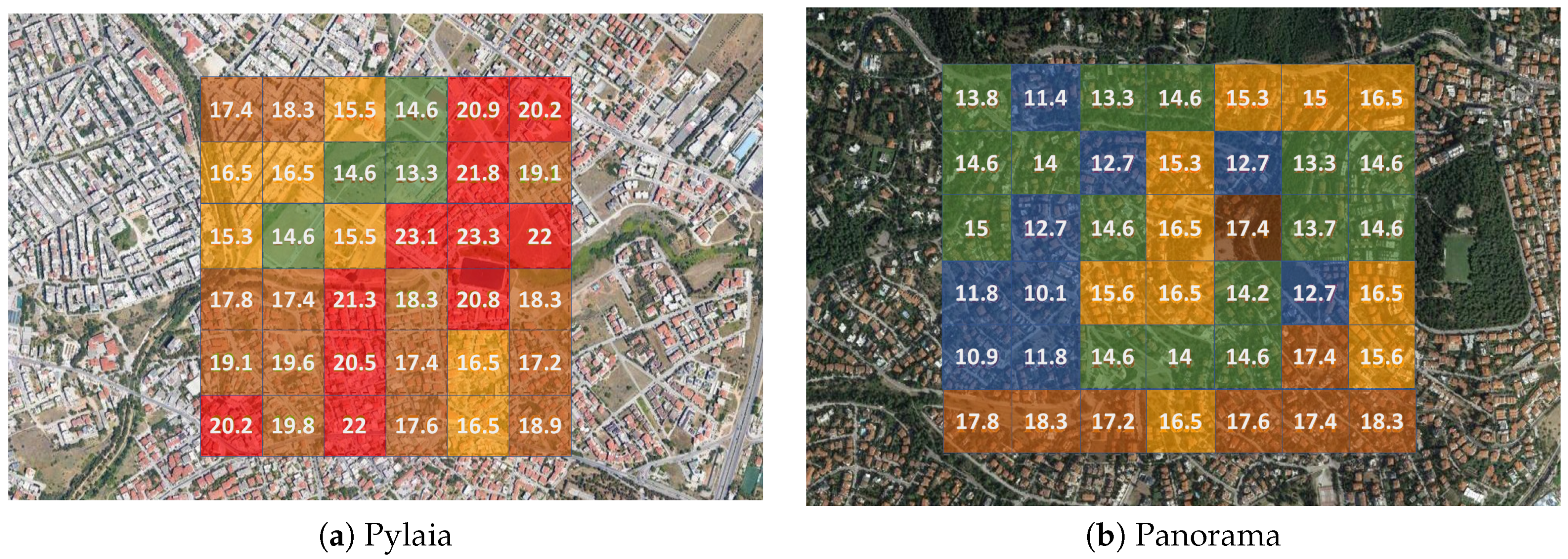
One of the benefits of using the proposed image-based surrogate is that it becomes possible to use the model to estimate SES indicators at high geographical resolution. Thus, although the Greek statistical authority publishes unemployment rates at municipality level (including populations of tens or even hundreds of thousands), we can attempt to estimate its value at neighborhood level, inside each municipality. This section demonstrates an example result of this type of estimation.

We selected two regions inside the municipality of Pylaia-Chortiatis (unempl. rate: 14.9%). One region is in the Pylaia area and the other is in the Panorama area. Although these two regions are in close proximity, Panorama has a fair amount of medium to high income residents, and is considered one of the highest SES areas of Thessaloniki. It includes a large number of detached houses and is not densely built. Pylaia, on the other hand, is considered to be lower SES than Panorama. A part of the Pylaia area includes apartment blocks and is more densely built. We wanted to observe whether the results of our model would agree with these qualitative observations, so we measured the surrogate variable and applied our model to blocks in these two areas. The results are visually illustrated in Figure 5.

Visual inspection indicates that (i) Panorama has a lower estimated unemployment rate (i.e., higher SES) than Pylaia and (ii) levels of unemployment rate are “grouped” into area connected components. Although we don’t have the means to directly validate the unemployment rate estimates, the results are consistent with our perception about these two areas and therefore provide an indication that estimating SES indicators at neighborhood level using image-based surrogates is possible.

4.4. Extension to Other SES Indicators

So far, our analysis has been limited to unemployment rate, which we consider to be a representative local SES indicator (average income would also be very informative, but this information is not publicly available at municipality level in Greece). To examine whether the proposed methodology can be extended to additional indicators, we used the proposed surrogate variable to build linear models that predict (a) the percentage of the employed population with higher executive positions (i.e., directors, administrators, and other high-level executives) and (b) the percentage of the employed population with university education at graduate or postgraduate level. A summary of the results (including unemployment rate, for comparison) is shown in

Table 6. Model effectiveness for three different Socio-Economic Status (SES) indicators.

ID	Indicator	${\mathit{R}}^2$	MAE (Test)	MAPE (Test)
1	Unemployment rate	$0.7635$	$1.87$	$0.089$
2	% of employed population with executive positions	$0.8653$	$0.88$	$0.1492$
3	% of employed population with university education	$0.8075$	$3.99$	$0.1094$

. Values have been computed using the same methodology as described previously.

According to these results, indicators 2 and 3 produce a more effective model (better $R^2$) but perform slightly worse in the held-out test municipalities. Note that although MAPE in the test set for the 2nd indicator is significantly worse ($0.1492$) the MAE is low ($0.88$). Overall, similar conclusions regarding the effectiveness of the proposed approach can be drawn for all three indicators, showing that the image-based surrogate methodology is not limited to unemployment rate only.

5. Conclusions

We have presented a fully automated methodology for estimating local SES indicators such as unemployment rate based on images acquired via Google Street View, without the need for any training labels. To achieve this, we built models that classify detected cars using multiple instance learning, where each detected car inherits the label of the municipality it was observed in (“high” or “low” SES). These models are used to produce variables that act as surrogates of SES indicators.

We applied our model and methodology in 30 municipalities in Greece and have shown that the results are satisfactory for several applications, achieving $R^2=0.76$ and a correlation coefficient of $0.874$ for the 25 municipalities used for building our linear regression model and $MAPE=0.089$, $MAE=1.87$ for a held-out test set of five municipalities. We also qualitatively evaluated the effectiveness of our model in estimating unemployment rate at neighborhood level in two areas inside the same municipality in the Thessaloniki region, where the results are consistent with our perception about the SES of these areas. Finally, we evaluated whether the proposed approach can be extended to other SES indicators related to occupational prestige and education level with encouraging results.

In terms of computational complexity, the proposed method requires heading computation by querying the Google geocoding API and image acquisition through Google GSV (the whole procedure took approximately 0.5 s per image on average in our experiments). Detection and classification of cars with Faster R-CNN largely depends on the available hardware (typical GPU implementation values are approximately 0.5 s per image). After that, the time for computing the surrogate variable is negligible. Our method therefore scales well and can be applied to large geographical regions with limited computational resources.

In our experiments, our model was shown to be most effective up to an unemployment rate of 24%. After that point, the surrogate (that relies on detected cars) was not able to discriminate between different unemployment rates. This hints that an improved model could perhaps be produced if additional objects, besides cars, or even image features (similarly to Reference [32]) are used for surrogate computation. This is one of our directions for future work in this area.

One additional question that we have not answered yet is the effectiveness of our methodology for different countries around the world. Given the differences in the publicly available statistics, in car models, as well as weather and lighting conditions across different countries, we expect that different models will need to be built for each country (which is straightforward, assuming an initial set of SES indicators at municipality level is available). Additionally, for some countries where cars are not commonly parked on the streets, moving cars will need to be taken into account. Exploring all these questions is the subject of future research.

Despite these remaining questions, the results that are presented in this work sufficiently demonstrate that the proposed image-based methodology can be used to provide good estimates of SES indicators at high geographical resolution, to support cost-effective, evidence-based decisions that take into account the local socioeconomic context of the population.