Review

An Overview of Watershed Algorithm Implementations in Open Source Libraries

National Research Nuclear University MEPhI, Kashirskoye sh. 31, 115409 Moscow, Russia
*
Author to whom correspondence should be addressed.
J. Imaging 2018, 4(10), 123; https://doi.org/10.3390/jimaging4100123
Submission received: 28 September 2018 / Revised: 16 October 2018 / Accepted: 17 October 2018 / Published: 20 October 2018

Abstract

:
Watershed is a widespread technique for image segmentation. Many researchers apply the method implemented in open source libraries without a deep understanding of its characteristics and limitations. In the review, we describe benchmarking outcomes of six open-source marker-controlled watershed implementations for the segmentation of 2D and 3D images. Even though the considered solutions are based on the same algorithm by flooding having O(n)computational complexity, these implementations have significantly different performance. In addition, building of watershed lines grows processing time. High memory consumption is one more bottleneck for dealing with huge volumetric images. Sometimes, the usage of more optimal software is capable of mitigating the issues with the long processing time and insufficient memory space. We assume parallel processing is capable of overcoming the current limitations. However, the development of concurrent approaches for the watershed segmentation remains a challenging problem.

1. Introduction

Segmentation of a digital image is the process of its division into a number of disjoint regions, so that pixels of every region have similar visual characteristics. The goal is to simplify or change the representation of an image for its further analysis. This is one of the most important tasks in pattern recognition and classification [1], visualization [2,3], image compression based on objects of interest [4,5], etc.
One of most common segmentation algorithms used in processing medical [6,7] and material science images [8,9] is a watershed algorithm. It is based on the representation of a grayscale image as a topographic relief, flooded with water, where watersheds are lines dividing areas of the water from different basins [10]. After its first proposal [11,12], this approach has developed significantly [13,14,15,16,17]. There are many scientific and industrial investigations that apply open source software for image processing. For instance, ref. [18,19] mention the watershed algorithm from the Insight Segmentation and Registration Toolkit (ITK) library for brain extraction from magnetic resonance images and analysis of glass foams using X-ray microtomography; ref. [20,21] mention the algorithm from the OpenCV library for counting of colonies to quantitate bacteria and malaria detection of drawing blood cells; ref. [22,23] mention the algorithm from the Mahotas library for a deep structured learning method for neuron segmentation from 3D electron microscopy and tracking of surface-labeled cells in time-lapse image sets of living tissues; ref. [24,25] mention the algorithm from the scikit-image (Skimage) library for pore network extraction from tomographic images and analyzing microtomography data.
Frequently, researchers use functions from open source software without deep understanding of the algorithms’ details and limitations. Sometimes, they have no information about alternative solutions. This can lead to worse performance in their investigations, as well as in developed software tools. The aims of our review are theoretical analysis of watershed algorithm implementations in open source software and performing processing time and memory consumption comparative estimations for the functions under analysis.
We searched mathematical morphology libraries that are widely used in practice for watershed segmentation and provide a call interface on the Python programming language and the lesser known alternatives. For this search of the libraries themselves and their documentation, we used Google and GitHub search engines, but also an IEEE Xplore database and the Google Scholar engine for papers that describe the practically used libraries for watershed segmentation, as well as the implementations of their algorithms. As information sources, we used English papers from conferences, journals, books and libraries’ documentation that were published from 1970–2018. We checked them for eligibility with the criteria: the libraries are available, not proprietary software and have the Python call interface, as well as data for analysis are available. You can see them in the References of this paper.
We deal with the watershed segmentation algorithms implemented in the following open source software libraries: Insight Segmentation and Registration Toolkit (ITK) [26], Open Source Computer Vision Library (OpenCV) [27], Mahotas [28], the Mathematical Morphology Image Library (Mamba) [29], scikit-image (Skimage) [30] and the Simple Morphological Image Library (SMIL) [31]. There is also a widely-used open source library, ImageJ [32], which does not provide the Python call interface, but it contains several implementations of watershed segmentation [33]. Furthermore, there is the Pink library [34], which contains implementations of two watershed algorithms [35,36].
Our contributions are the following: providing a list of available software for watershed segmentation; a description of the algorithms in the software and experimental estimation of their performance; analysis of the limitations for processing of huge images. Sometimes, the usage of more optimal software is capable of mitigating the issues with long processing time and insufficient memory space.
This review is organized as follows: Section 2 describes the main approaches of watershed segmentation; Section 3 describes the algorithms currently used in open source software libraries; Section 4 presents the measured dependence of execution time and maximum amount of memory on the sizes of the test images, as well as gives the average execution time per one image element; Section 5 contains the discussion about the current state of affairs in solving the problem of image segmentation by the implementation of the watershed algorithm presented in open source libraries.

2. Main Approaches of Watershed Segmentation

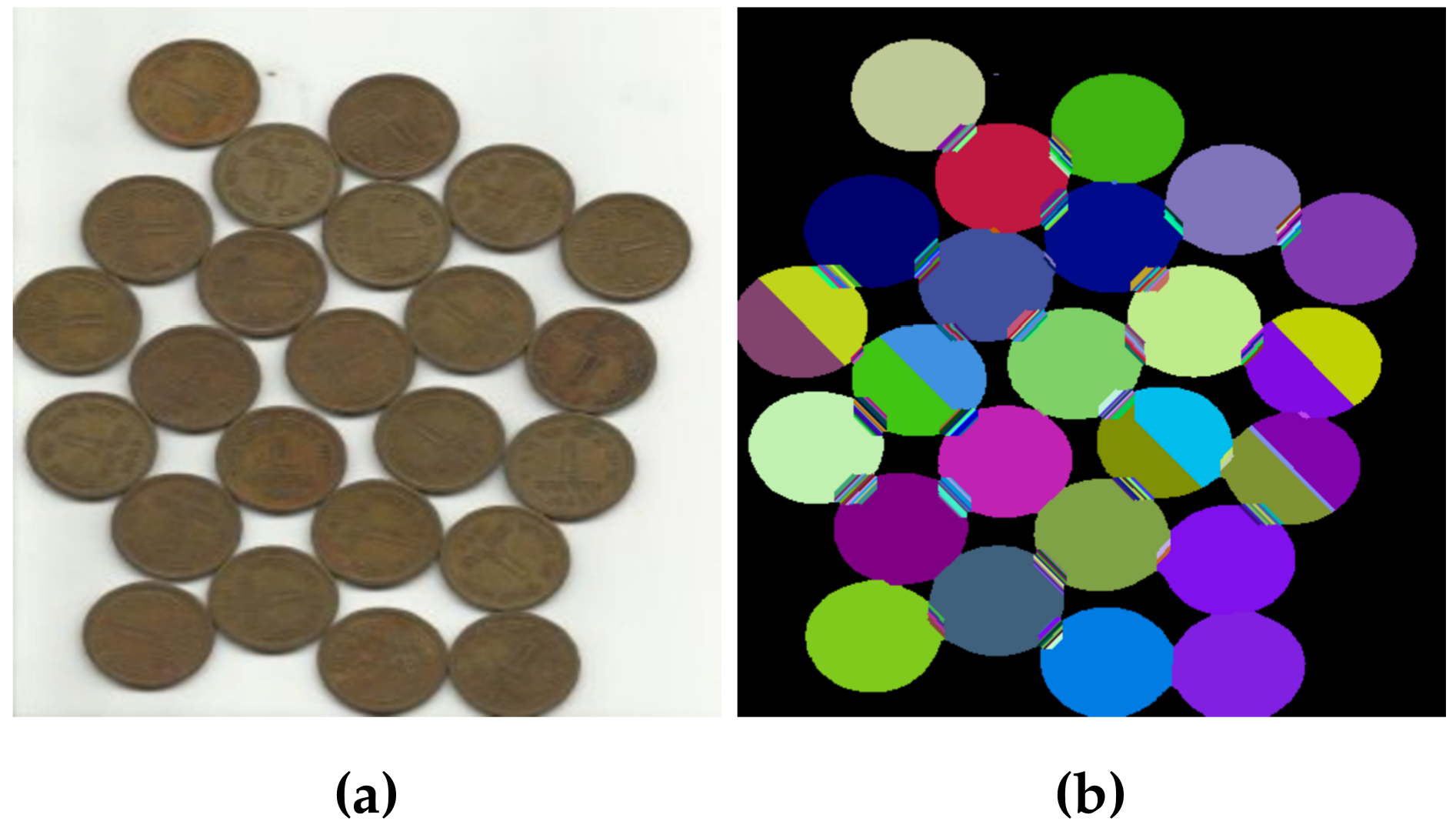
The watershed segmentation algorithms are based on the representation of an image in the form of a topographic relief, where the value of each image element characterizes its height at this point. These algorithms can process not only 2D images, but also 3D images, so the term element is used in the paper to combine the terms pixel and voxel. For a better outcome, watershed segmentation is often applied to the result of the distance transform of the image rather than to the original one [7,37]. Thus, the relief consists of low-lying valleys (minimums), high-altitude ridges (watershed lines) and slopes (catchment basins). The concept of plateau (an area with the same height of elements) is also used. The main task in this segmentation method is to determine the location of all catchment basins and/or watershed lines, since in this case, each catchment basin is considered to be a separate segment of the image. In some tasks, we only need to get the segments, but in some, we also need to know the boundaries of each segment. Accordingly, watershed algorithms with and without watershed line construction were proposed. In Figure 1, we can see the differences in the result of segmentation with and without the watershed line construction, the line that divides the two final segments. There are two main approaches to finding these watersheds: by flooding and by rain falling [35,38].

2.1. Watershed by Flooding

This approach was initially proposed by Vincent and Soille [15]. It realizes the following: ‘Holes are pierced’ in every minimum, and the entire relief begins to be flooded with water. Starting from the minimum of lowest height, the water gradually fills up all catchment basins. Watersheds are built in the places where water from different basins unites. The process ends when the water reaches the maximum peak of the relief, and as a result, every catchment basin gets covered by the watershed lines.
To simulate this process, the algorithms proposed by Beucher and Meyer are used the most often, and the first of them consists of the following steps [35]:
A1
We find the local minima in the image. Each of them is assigned with a unique marker.
A2
We simulate a flooding process that uses a priority queue that consists of H queues, where H is the number of possible image element values (for example, H = 256 if the gray level varies from 0–255). When it is filled, the elements of the image with the value of h are pushed into the corresponding queue with the number h.
(a)
We fill the priority queue with the elements of image local minima.
(b)
We scan the priority queue in sequence from smaller values of h to larger ones. Then, we select the element from the first non-empty queue. If all queues from the priority queue are empty, the algorithm terminates.
(c)
We remove the selected element from the queue, and its marker propagates on all unmarked neighbors.
(d)
We place all the neighbors marked in the previous step into the priority queue. Then, we proceed to Step A2.
The result will not contain the watershed lines in this case. If they are required, the second approach is applied [39]:
B1
Similar to Step A1.
B2
A similar priority queue is used, as described in Step A2. Furthermore, each element of the image needs to be marked additionally, depending on whether it was already placed into this queue or not (an additional marker).
(a)
We mark elements, that already have a unique marker, with an additional marker.
(b)
Into the priority queue, we add elements that have marked neighbors. We also mark them with an additional marker.
(c)
Similar to Step A2.
(d)
We remove the selected element from the queue. If all its marked neighbors were marked with the same marker, we mark the element itself by this marker. If the selected element was a neighbor of elements with different markers, we mark it with a special marker, meaning that it is an element of the watershed.
(e)
Neighbors of this element that have not been marked with an additional marker yet are placed into the priority queue. Then, we proceed to Step B2c.

2.2. Watershed by Rain Falling

Another approach, based on connectivity components and modeling the rain process, was proposed by Bieniek and Moga [38]. The basic idea is that a drop of water after falling onto the surface of the image relief flows down along the slope to the corresponding valley. The path along which the drop drips is called the connectivity component and also is the steepest path between the point of the fall and the valley. All connected components that lead to the same valley form one catchment basin. For images that contain only minimal plateaus, the present algorithm requires only three complete passes of the image. However, since images usually contain non-minimal plateaus, an additional step with one more full pass is required, as well as an additional queue. Thus, the algorithm marks all the catchment basins with only four full passes of the image.
The classical algorithm consists of the following steps:
C1
Pass 1. We mark each element of the image with the location of a lower adjacent element, which has the smallest value (usually realized with pointers). If there are no such elements in the neighborhood, then the current one is marked as an element of the plateau.
C2
Elimination of non-minimal plateaus.
(a)
Pass 2. We check the neighbors for each element that is marked as a plateau. If among them we find one that is not marked as a plateau and has the same value as the element itself, we push this neighbor into the queue and complete the check of the neighbors for this element.
(b)
While the queue of neighbors is not empty, we remove the elements from it. We check their neighbors that are marked as a plateau. We mark them with markers pointing to the location of the removed element and push them all into the queue.
C3
Pass 3. We mark the minimum plateau elements with representative values.
(a)
First, we mark each element that is marked as a plateau with a marker that points on the element itself.
(b)
Sequentially, we take the neighbors of the current element, which have already been passed and have the same value.
For the current element and this neighbor, we perform a path compression procedure. It consists of traversing the path using markers as motion pointers, from the given element to that marked with a marker pointing to itself, and then assigning to each marker of the path elements the value of the marker of the finite element on it.
After these procedures, we mark the end elements of these compressed paths with a minimum value from their markers.
C4
Pass 4. We perform the path compression procedure, described in Step C3b, for every image element. We mark elements with finite element markers of the path traversed by the compression procedure. The algorithm terminates.
The result of the given algorithm is the same as when using any traditional algorithm that does not create watershed lines. At the same time, it does not depend on the range of possible values of image elements, uses simple data structures and spends less runtime than algorithms based on flooding simulation [38].
It is worth noting that a number of works appeared aimed at theoretical and practical development of watershed optimized versions. For instance, a paper [40] extended a graph-based image segmentation framework and proposed a new family of algorithms termed power watersheds; a paper [41] proposed a novel evaluation framework that is used to optimize hierarchies for hierarchical watersheds.

2.3. Oversegmentation Problem

When applied to real images, the watershed transformation causes oversegmentation. This happens because in the standard approach, initial markers mark all local minima of the image. Therefore, each of the marked elements, and thus each of the local minima, becomes the center of the catchment basin, but not all of these minima are equally important. For example, some of them are formed due to noise, minor fluctuations in brightness and secondary image structures [37]. An example of oversegmentation is shown in Figure 2.
The solution to this problem is marking only significant parts of the original image and the limitation of the segmentation process in order to grow only one area around each marker. This method is called a marker-controlled watershed. There are two possible approaches: first [7,35], transform the image in such a way that regional minima will be located only in selected marker locations (usually done by morphological reconstruction), and then, apply the classical watershed algorithm; and second [42], execute the post-processing of an oversegmented image that connects each unmarked area with the nearest marked one, according to the accepted distance metric [43].

3. Implementations in Software Libraries

As mentioned earlier, in this paper, we overview the implementations used in libraries: ITK, OpenCV, Mahotas, Mamba, Skimage and SMIL. Despite the fact that this paper is aimed at overviewing implementations, an important property of a library is the activity of its development and updating. Therefore, at the moment, we can rank these libraries in the following order by the number of participants (in descending order): OpenCV, Skimage, ITK, Mahotas, SMIL, Mamba. Furthermore, we can rank these libraries by the ratio of the library lifetime to the number of its releases (in descending order): Mamba, SMIL, Mahotas, Skimage, OpenCV, ITK.
It should be noted that in some of the libraries, implementations automatically produce the initial marking of the image, but in this paper, we overview only those ones that allow one to assign it directly. The reason is that we compare the spent resources without the influence of initial marker obtaining step. Moreover, in practice, such implementations are used the most often. Table 1 shows some information on the implementations under review.
Despite a number advantages of the watershed algorithm implementations by rain falling over flooding model described in [38], they also have some significant drawbacks, due to which implementations by flooding are used in the examined program libraries. This is mainly due to non-minimal plateau: the impossibility of splitting them into several parts when using the approach by rain falling, which might better suit the physical nature of rain (for example, a ridge that should be divided in the middle). There is also a problem when marking several neighboring regions with equal height, while the model of flooding avoids these problems [44].
The ITK, Mahotas, Mamba, Skimage and SMIL libraries contain implementations of the watershed algorithms with the construction of watershed lines and without them, described in [44,45]. The OpenCV library gives an implementation of the modified algorithm for processing of color images with the watersheds construction, which is described below. The implementations of all libraries, except OpenCV, allow you to work with 3D images in addition to processing 2D images.
In the ITK, Mamba and SMIL libraries, both algorithms are implemented separately (with construction of watershed lines and without), while in Mahotas and Skimage, the implementations are combined into one. In addition, all implementations, except OpenCV, provide the opportunity to select the structural element of image connectivity. The Skimage library also provides an opportunity to build a compact watershed [46]. All implementations at the output produce the segments marking, as well as marking of watershed lines, if required. Some implementations combine markings into one and store them in one final array (ITK, OpenCV, Skimage), and some separate them into two (Mahotas, Mamba, SMIL).
Although these implementations are based on the algorithms with O ( n ) time complexity relative to the number of image elements, their time costs also strongly depend on the implementation language, applied software optimizations, asymptotic constant factors and other parameters [47]. For example, Luengo Hendriks [48] performed research of various priority queues in terms of performance and image analysis. In this work, the importance of selecting a good priority queue was demonstrated. For instance, execution time for the grey-weighted distance transform of a 3D image with 512 3 elements can be reduced from 40 to 20 min by using hierarchical heap rather than an AVLtree. Then, based on this paper, Barnes et al. [49] showed how the choice of different queues affects the performance of the priority-flood algorithm for digital elevation models and proposed their own optimal modification of the algorithm.
The OpenCV library implements the algorithm proposed by Meyer [50]. It is an extension of the watershed algorithm described in Section 2.1 (with the watershed line construction), for color RGB images segmentation. It introduces the following changes:
  • The maximum difference from all color channels is accepted as a measure of the difference between an element and its neighbors and as a measure of priority in the queue. If there are two elements x and y having the colors ( r x , g x , b x ) and ( r y , g y , b y ) , respectively, the difference is calculated by the following formula:
    d ( x , y ) = M a x | r x r y | , | g x g y | , | b x b y |
  • The priority queue size is selected according to the maximum possible difference between the color channels.
For natural images, this approach may give a better segmentation result, but if you segment contiguous objects with a similar size, the result may be worse than when using the distance transform. These advantages and disadvantages are due to the fact that the result depends on the color difference of the segmented objects. Furthermore, noise and minor color fluctuations significantly affect it. As an example, in Figure 3, you can see the segmentation results of such images by the OpenCV and Skimage implementations. Furthermore, this approach allows you to apply a watershed segmentation directly to a color image and get a higher resolution when segmenting color images than using a morphological gradient [51,52]. However, a better segmentation result could be obtained by using a uniform color metric [53].

4. Comparative Estimation

4.1. Test Images

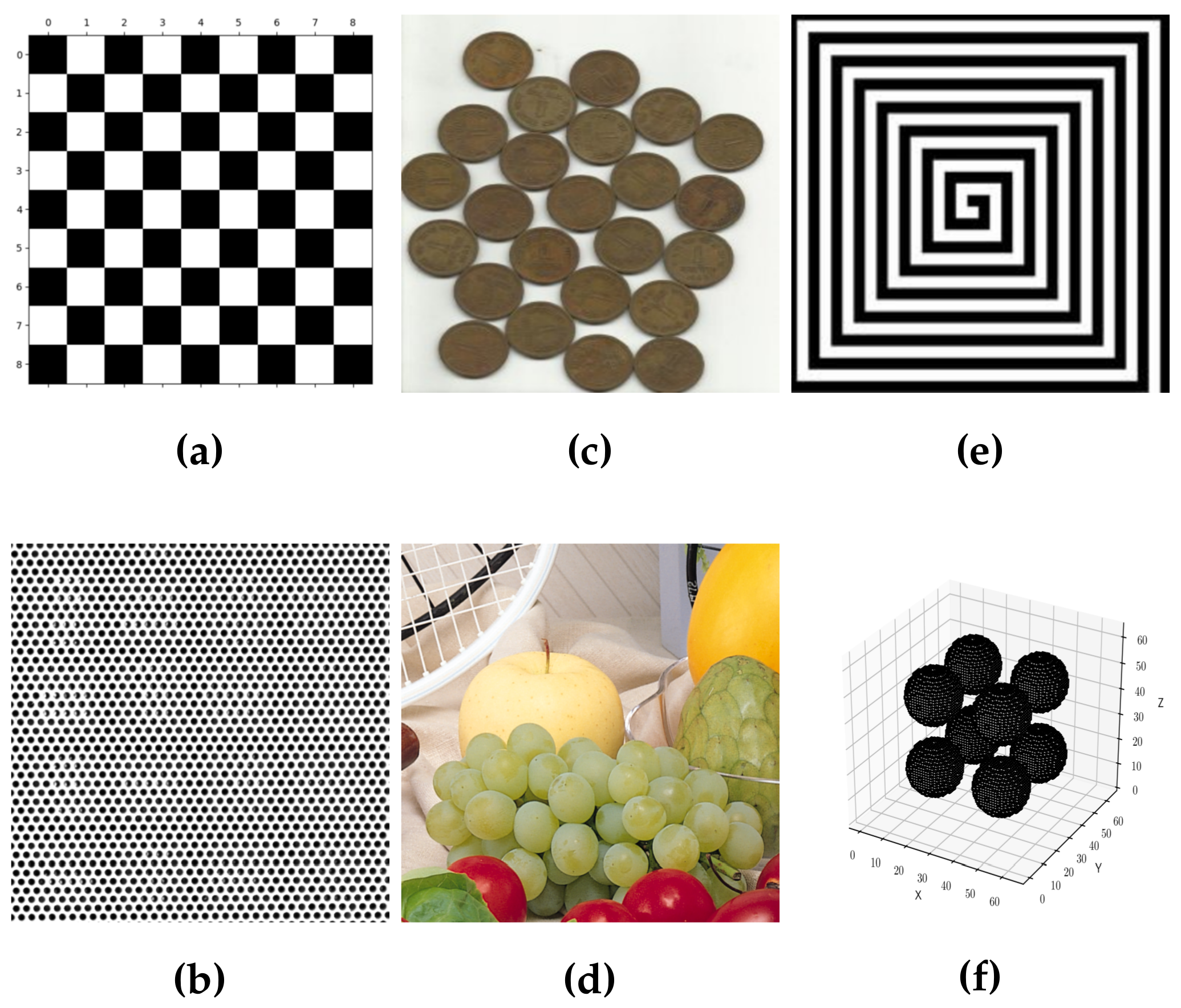
We measured the expended computing resources of segmentation, depending on the image size for a series of 2D images (board, cells, coins, fruits, maze) and the generated 3D image (balls), shown in Figure 4. These samples contain the following: images of objects with similar sizes, both with a relatively small number of objects (board, coins, balls) and with a relatively large one (cells); a natural image (fruits); and an artificial image with a snake-like structure (maze).
We applied the nearest-neighbor method for scaling each image to preserve their morphological relief. With this scaling method, the result of the distance transformation will be scaled in the same way. We chose images of a regular shape, and the dimensions for each axis were calculated by the following formula, where sz i is the image size on each coordinate axis, D is the number of image dimensions and st is the step of image size change.
sz i = sz 0 D + i · st D , i = 1 , 2 , . . . , N
In this paper, we used the following values: the step of image size change st = 4 × 10 5 elements, N = 40 for D = 2 and D = 3 and the initial image sizes sz 0 2 = 512 2 and sz 0 3 = 64 3 elements.
Some of the images were obtained from USC-SIPI [54] (cells), OpenCV tutorial [55] (coins), CAE University of Wisconsin [56] (fruits), and others were generated (board, maze, balls).

4.2. Description of Measurement Procedure

We used Python to measure the computational resources of the implementations, since all the examined libraries provide an interface for calling their functions in this language. We used a PC with an Intel Core i7-2600 CPU @ 3.40 GHz × 8 (Intel Corporation, Santa Clara, CA, USA), 8 GiB of RAM on GNU/Linux 4.17.3 x86-64 OS. The libraries were compiled using GCC 8.1.1 and were started by Python 3.6.4. The source code of testing scripts can be found on GitHub by following the URL: https://github.com/ant-Korn/Comparing_watersheds. However, there is a risk that the physical PC and OS may have different bit-length architectures.
We made measurements without taking into account the steps of generating input data of the algorithms. As the input, we used the result of inversed distance transformation on a binarized image (with the exception of OpenCV case, where we used the image itself) and the initial marking generated on the basis of this distance transform. We also used structural elements with full connectivity: a square one, connecting eight neighboring elements for 2D images, and a cubic one, connecting 26 neighboring elements for 3D, respectively. It should be noted that the implementation of OpenCV supports only the square structural element. All the other parameters of the algorithms were set to standard values. For each library, except OpenCV, we measured the computational resources of implementations for cases without generation of watershed lines (WL) and with them. We performed the measurements multiple times for each case, and then, we calculated the average of all the results to obtain the final value.

4.3. Results

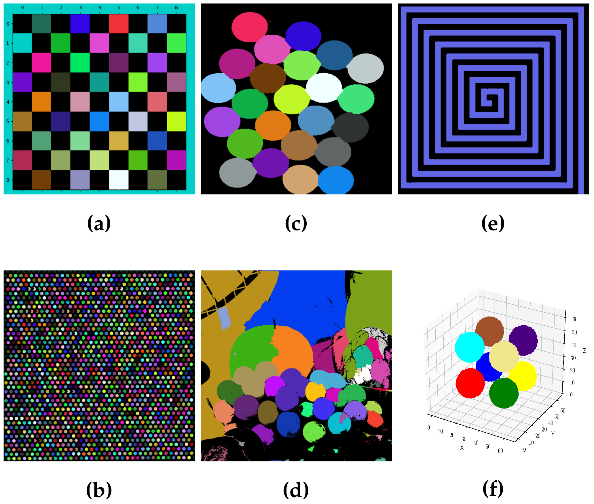
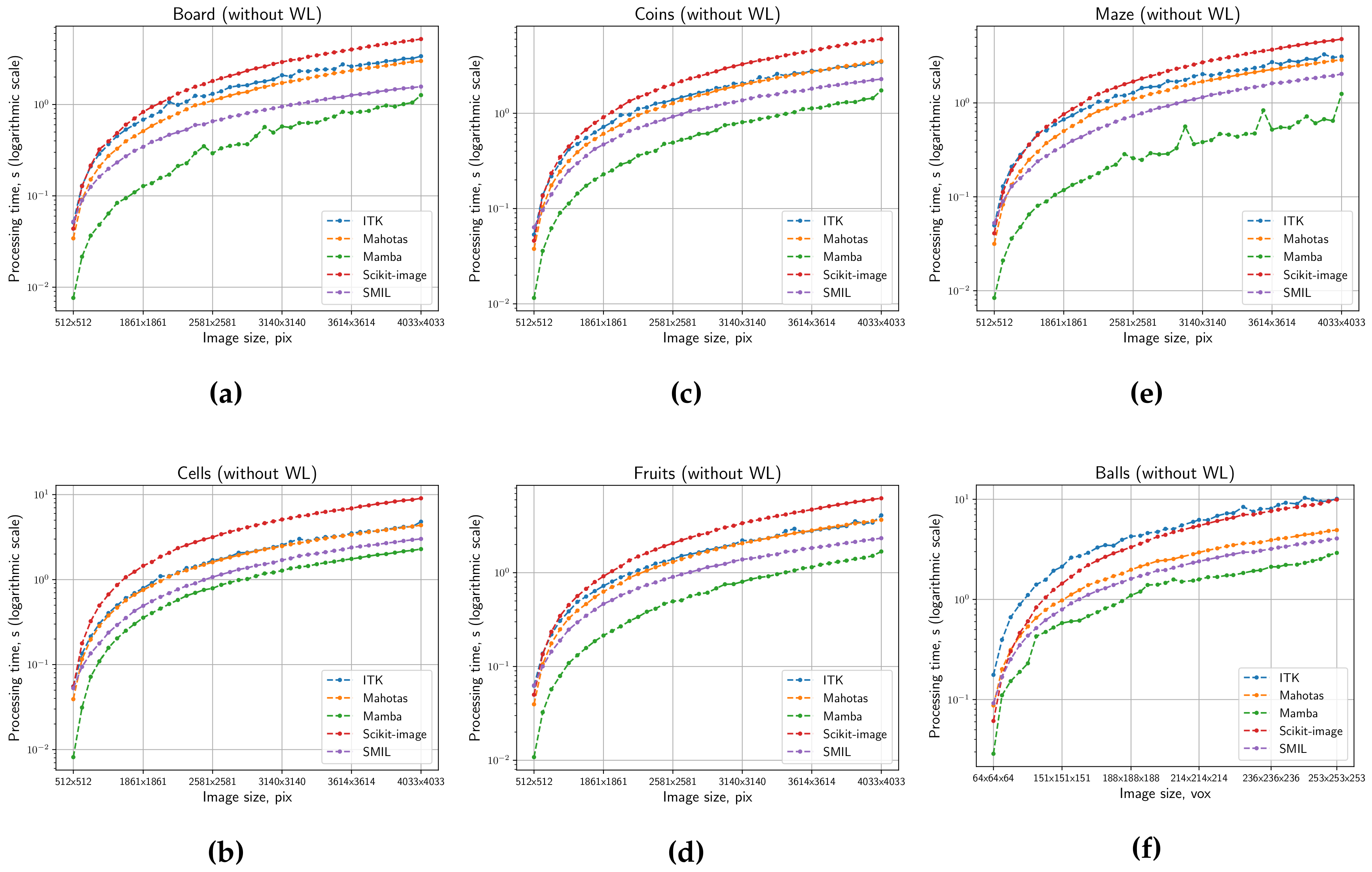
The each segmentation result of the initial size images is shown in Figure 5. On the basis of the experimental data, we plotted the dependence of the execution time on the images size: Figure 6 for images without the construction of WL and Figure 7 with it.
According to the presented graphs, we can see that the time complexity of each realized algorithm is really O ( n ) relative to the number of image elements. We can also see that, in terms of time efficiency, the OpenCV and Mamba implementations stand out against the background of other libraries. The first one showed the best results in segmenting 2D images with construction of watershed lines, and the second one in all other cases when the first one was not applicable.
For numerical comparison, we calculated the average time for processing one element by each implementation. Therefore, in Table 2, we present these values, calculated on the basis of all considered image sizes, for realizations without the construction of watershed lines, and in Table 3, respectively, with them.
From these experimental data, it follows that processing with the construction of watershed lines always requires more time than without it. Thus, we can conclude that in cases where the construction of watershed lines is not required, it is preferable to use appropriate implementations. Furthermore, we can see the dependence of the execution time on the number of initial markers and the sizes of the resulting segments areas. In the case of using the not most optimized implementation, the processing can require much more time: for 2D images, on average, 1.8 4.5 -times more for the case without WL and 2.4 42 -times more for the case with WL, for 3D 1.5 3.9 times more and 1.2 41 -times more, respectively, depending on the selected library.
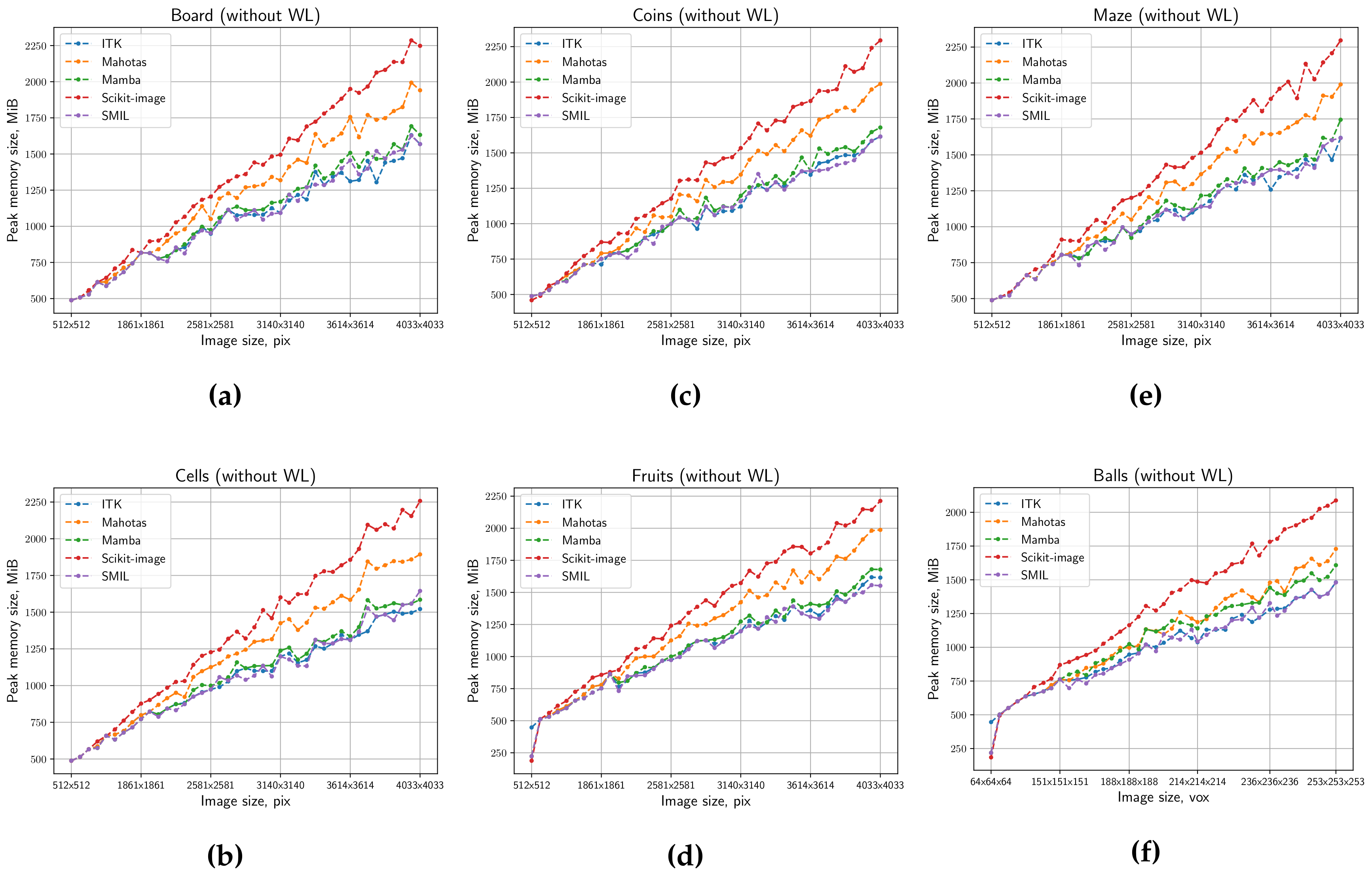
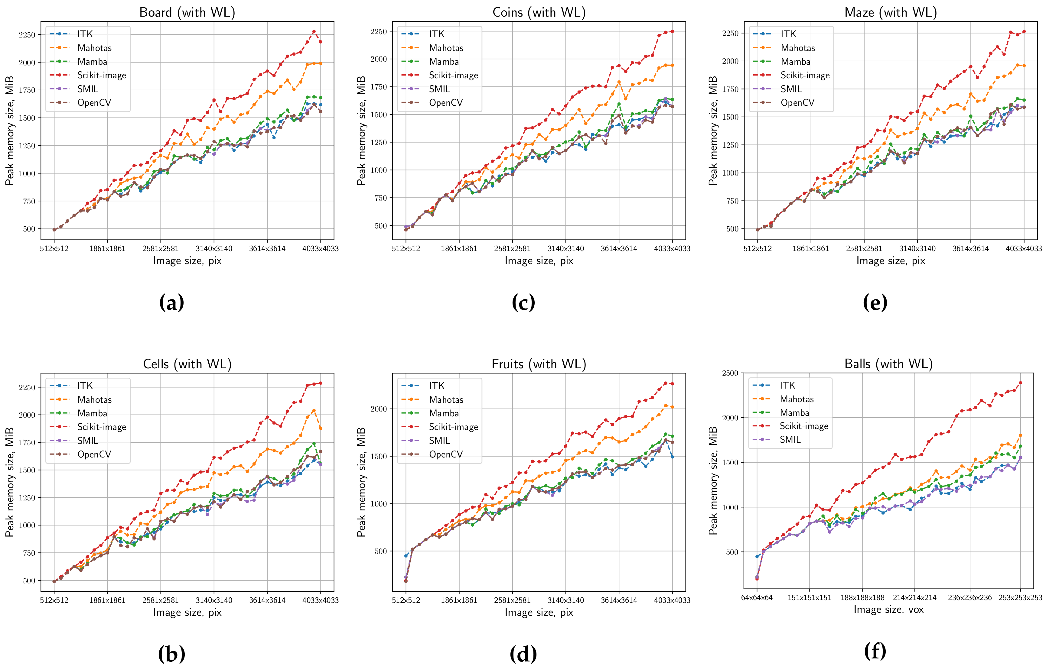
In addition, we measured the peak memory volume used by each implementation. The corresponding graphs are presented in Figure 8 for images without the construction of WL and Figure 9 with the construction. We can see from these graphs that the implementations of all libraries, with the exception of Skimage, Mahotas for the 2D case and Skimage for the 3D case, use a similar peak memory volume in both cases. Therefore, most of the implementations showed similar results with a difference of 2% for the 2D case and 7% for 3D. The only exception is the implementations that had larger peak memory consumption on average: Mahotas by 9% and Skimage by 18% for the 2D case; Skimage by 16% without construction of WL and 27% with construction of WL for the 3D case.
When using other hardware, the result may be different, but the ratio of the results in most cases should be preserved. If newer versions of the libraries are used, the result values may increase or decrease depending on the applied software optimizations or errors. Furthermore, more optimized implementations can possibly be found in other libraries that do not support the Python call interface or are proprietary software.

5. Discussion

In this paper, we have overviewed and measured the expended computational resources of the watershed segmentation algorithms that are implemented in some open source libraries. Despite the fact that most of them implement the same algorithms with O ( n ) time complexity relative to the number of image elements, empirical testing shows a large difference in execution time, since it also depends on many other factors, such as implementation language, applied software optimizations, etc. Furthermore, most libraries showed similar results in the peak memory consumption. We identified two libraries that showed the best results in our tests. Thus, for the best performance of the watershed segmentation, one should try different implementations from modern versions of libraries and choose the one that consumes the least computing resources, despite the fact that most of them contain implementations of the same algorithms. With this testing, one can already achieve a significant increase in performance.
Frequently, computational power and available memory can be bottlenecks for processing of huge images, which is especially true for the 3D case [7,8,57]. A good example is provided by X-ray microtomography images of sizes 1024 × 1024 × 1000 , 2048 × 2048 × 1000 and 4000 × 4000 × 2000 that are used for the analysis of mineral particles [58,59,60]. In a natural way, dealing with such huge 3D images requires rather large computational resources. For example, since the computational complexity is linear, 1.4 h and 2 TiB would be spent on the segmentation of the presented 3D image with a size of 4000 × 4000 × 2000 (by the Mamba implementation without WL construction on the presented hardware). For this reason, there have been many proposals for the parallelization of the watershed algorithm [43,61,62,63,64,65,66,67,68], but a significant result was difficult to achieve because of its sequential nature [69]. For some problems, when memory becomes a crucial issue, the only appropriate solution is splitting of the initial image into smaller parts, segmenting of these parts in parallel and following the merging of results. Even in this case, the performance of the segmentation algorithm implementation plays a significant role, since each part of the image must be processed with minimal computational resources.

Author Contributions

Conceptualization, A.S.K. and I.V.S. Methodology, A.S.K. and I.V.S. Software, A.S.K. Validation, A.S.K. and I.V.S. Formal analysis, A.S.K. and I.V.S. Investigation, A.S.K. Resources, I.V.S. Data curation, A.S.K. Writing, original draft preparation, A.S.K. Writing, review and editing, A.S.K. and I.V.S. Supervision, I.V.S.

Funding

This research received no external funding.

Conflicts of Interest

The authors declare no conflict of interest.

Abbreviations

The following abbreviations are used in this manuscript:
2DTwo-dimensional
3DThree-dimensional
WLWatershed lines

References

  1. Suetens, P.; Fua, P.; Hanson, A.J. Computational Strategies for Object Recognition. ACM Comput. Surv. 1992, 24, 5–62. [Google Scholar] [CrossRef]
  2. Bomans, M.; Hohne, K.H.; Tiede, U.; Riemer, M. 3-D segmentation of MR images of the head for 3-D display. IEEE Trans. Med. Imaging 1990, 9, 177–183. [Google Scholar] [CrossRef] [PubMed]
  3. McAuliffe, M.J.; Lalonde, F.M.; McGarry, D.; Gandler, W.; Csaky, K.; Trus, B.L. Medical Image Processing, Analysis and Visualization in clinical research. In Proceedings of the 14th IEEE Symposium on Computer-Based Medical Systems, CBMS 2001, 26–27 July 2001; pp. 381–386. [Google Scholar]
  4. Hsu, W.Y. Segmentation-based compression: New frontiers of telemedicine in telecommunication. Telemat. Inf. 2015, 32, 475–485. [Google Scholar] [CrossRef]
  5. Natale, F.G.B.D.; Desoli, G.S.; Giusto, D.D.; Vernazza, G. Polynomial approximation and vector quantization: a region-based integration. IEEE Trans. Commun. 1995, 43, 198–206. [Google Scholar] [CrossRef]
  6. Pham, D.L.; Xu, C.; Prince, J.L. Current Methods in Medical Image Segmentation. Annu. Rev. Biomed. Eng. 2000, 2, 315–337. [Google Scholar] [CrossRef] [PubMed]
  7. Atta-Fosu, T.; Guo, W.; Jeter, D.; Mizutani, C.M.; Stopczynski, N.; Sousa-Neves, R. 3D Clumped Cell Segmentation Using Curvature Based Seeded Watershed. J. Imaging 2016, 2, 31. [Google Scholar] [CrossRef] [PubMed]
  8. Waggoner, J.; Zhou, Y.; Simmons, J.; Graef, M.D.; Wang, S. 3D Materials Image Segmentation by 2D Propagation: A Graph-Cut Approach Considering Homomorphism. IEEE Trans. Image Process. 2013, 22, 5282–5293. [Google Scholar] [CrossRef] [PubMed]
  9. Myasnikov, E.V. Hyperspectral image segmentation using dimensionality reduction and classical segmentation approaches. Comput. Opt. 2017, 41, 564–572. [Google Scholar] [CrossRef]
  10. Serra, J. Image Analysis and Mathematical Morphology; Academic Press: New York, NY, USA, 1982. [Google Scholar]
  11. Digabel, H.; Lantuéjoul, C. Iterative algorithms. In Actes du Second Symposium Européen d’Analyse Quantitative des Microstructures en Sciences des Matériaux, Biologie et Médecine, Caen, 4–7 October 1977; Chermant, J.L., Ed.; Dr. Riederer: Stuttgart, Germany, 1978; pp. 85–99. [Google Scholar]
  12. Lantuéjoul, C. La Squelettisation et son Application aux Mesures Topologiques des Mosaques Polycristallines. Ph.D. Thesis, Ecole des Mines, Paris, France, 1978. [Google Scholar]
  13. Beucher, S.; Lantuéjoul, C. Use of Watersheds in Contour Detection. In Proceedings of the International Workshop on Image Processing: Real-time Edge and Motion Detection/Estimation, Rennes, France, January 1979; Volume 132. [Google Scholar]
  14. Meijster, A.; Roerdink, J.B.T.M. A proposal for the implementation of a parallel watershed algorithm. In Computer Analysis of Images and Patterns: 6th International Conference, CAIP ’95 Prague, Czech Republic, September 6–8, 1995 Proceedings; Hlaváč, V., Šára, R., Eds.; Springer: Berlin/Heidelberg, Germany, 1995; pp. 790–795. [Google Scholar]
  15. Vincent, L.; Soille, P. Watersheds in digital spaces: An efficient algorithm based on immersion simulations. IEEE Trans. Patt. Anal. Mach. Intell. 1991, 13, 583–598. [Google Scholar] [CrossRef]
  16. De Smet, P.; Pires, R. Implementation and analysis of an optimized rainfalling watershed algorithm. In Proceedings of the SPIE, VCIP’2000, San Jose, CA, USA, 19 April 2000; Volume 3974, pp. 759–766. [Google Scholar]
  17. Meyer, F. Topographic distance and watershed lines. Signal Process. 1994, 38, 113–125. [Google Scholar] [CrossRef]
  18. Beare, R.; Chen, J.; Adamson, C.L.; Silk, T.; Thompson, D.K.; Yang, J.Y.M.; Anderson, V.A.; Seal, M.L.; Wood, A.G. Brain extraction using the watershed transform from markers. Front. Neuroinf. 2013, 7, 1–15. [Google Scholar] [CrossRef] [PubMed]
  19. Atwood, R.; Jones, J.; Lee, P.; Hench, L. Analysis of pore interconnectivity in bioactive glass foams using X-ray microtomography. Scr. Mater. 2004, 51, 1029–1033. [Google Scholar] [CrossRef]
  20. Wong, C.F.; Yeo, J.Y.; Gan, S.K.E. APD Colony Counter App: Using Watershed algorithm for improved colony counting. Nat. Methods Appl. Notes 2016, 1–3. [Google Scholar] [CrossRef]
  21. Herusutopo, A.; Bisono, R.W.; Meliala, J.I. Application Of Malaria Detection Of Drawing Blood Cells Using Microscopic Opencv. Commun. Inf. Technol. J. 2011, 5, 65–73. [Google Scholar] [CrossRef]
  22. Funke, J.; Tschopp, F.; Grisaitis, W.; Sheridan, A.; Singh, C.; Saalfeld, S.; Turaga, S.C. A Deep Structured Learning Approach Towards Automating Connectome Reconstruction from 3D Electron Micrographs. arXiv, 2017; arXiv:1709.02974. [Google Scholar]
  23. Mashburn, D.N.; Lynch, H.E.; Ma, X.; Hutson, M.S. Enabling user-guided segmentation and tracking of surface-labeled cells in time-lapse image sets of living tissues. Cytometry A 2012, 81A, 409–418. [Google Scholar] [CrossRef] [PubMed]
  24. Gostick, J.T. Versatile and efficient pore network extraction method using marker-based watershed segmentation. Phys. Rev. E 2017, 96, 023307. [Google Scholar] [CrossRef] [PubMed]
  25. Gouillart, E.; Nunez-Iglesias, J.; van der Walt, S. Analyzing microtomography data with Python and the scikit-image library. Adv. Struct. Chem. Imaging 2016, 2, 18. [Google Scholar] [CrossRef] [PubMed]
  26. Johnson, H.J.; McCormick, M.; Ibáñez, L.; Consortium, T.I.S. The ITK Software Guide, 4th ed.; Kitware, Inc.: New York, NY, USA, 2018. [Google Scholar]
  27. Bradski, G. The OpenCV Library. Dr. Dobb’s J. Softw. Tools 2000, 122–125. [Google Scholar]
  28. Coelho, L.P. Mahotas: Open source software for scriptable computer vision. J. Open Res. Softw. 2013, 1, e3. [Google Scholar] [CrossRef]
  29. Beucher, N.; Beucher, S. Mamba Image User Manual. 2017. Available online: http://mamba-image.org/docs/2.0/mamba-um.pdf (accessed on 28 September 2018).
  30. Van der Walt, S.; Schönberger, J.L.; Nunez-Iglesias, J.; Boulogne, F.; Warner, J.D.; Yager, N.; Gouillart, E.; Yu, T.; The Scikit-Image Contributors. Scikit-image: Image processing in Python. PeerJ 2014, 2, e453. [Google Scholar] [CrossRef] [PubMed]
  31. Simple Morphological Image Library. Available online: http://smil.cmm.mines-paristech.fr (accessed on 28 September 2018).
  32. Rueden, C.T.; Schindelin, J.; Hiner, M.C.; DeZonia, B.E.; Walter, A.E.; Arena, E.T.; Eliceiri, K.W. ImageJ2: ImageJ for the next generation of scientific image data. BMC Bioinform. 2017, 18, 529. [Google Scholar] [CrossRef] [PubMed] [Green Version]
  33. Legland, D.; Arganda-Carreras, I.; Andrey, P. MorphoLibJ: Integrated library and plugins for mathematical morphology with ImageJ. Bioinformatics 2016, 32, 3532–3534. [Google Scholar] [CrossRef] [PubMed]
  34. Couprie, M.; Marak, L.; Talbot, H. The pink image processing library. In Proceedings of the Poster European Python Scientific Conference, Austin, TX, USA, 11–16 July 2011. [Google Scholar]
  35. Beucher, S.; Meyer, F. The morphological approach to segmentation: The watershed transformation. In Mathematical Morphology in Image Processing; Marcel Dekker Inc.: New York, NY, USA, 1993; Volume 34, Chapter 12; pp. 452–464. [Google Scholar]
  36. Couprie, M.; Bertrand, G. Topological Grayscale Watershed Transformation. In Proceedings of the SPIE Vision Geometry V, San Diego, CA, USA, 27 July–1 August, 20 October 1997; Volume 3168, pp. 136–146. [Google Scholar]
  37. Safonov, I.V.; Mavrin, G.N.; Kryzhanovsky, K.A. Segmentation of Convex Cells with Partially Undefined Edges. Pattern Recognit. Image Anal. 2008, 18, 112–117. [Google Scholar] [CrossRef]
  38. Bieniek, A.; Moga, A. An efficient watershed algorithm based on connected components. Pattern Recognit. 2000, 33, 907–916. [Google Scholar] [CrossRef]
  39. Meyer, F. Un algorithme optimal de ligne de partage des eaux. In Proceedings of the 8th Congress AFCET, Lyon-Villeurbanne, France, 25–20 November 1991; Volume 2, pp. 847–859. [Google Scholar]
  40. Couprie, C.; Grady, L.; Najman, L.; Talbot, H. Power watersheds: A new image segmentation framework extending graph cuts, random walker and optimal spanning forest. In Proceedings of the 2009 IEEE 12th International Conference on Computer Vision, Kyoto, Japan, 27 September–4 October 2009; pp. 731–738. [Google Scholar]
  41. Perret, B.; Cousty, J.; Guimarães, S.J.; Maia, D.S. Evaluation of Hierarchical Watersheds. IEEE Trans. Image Process. 2018, 27, 1676–1688. [Google Scholar] [CrossRef] [PubMed] [Green Version]
  42. Meyer, F. Minimum Spanning Forests for Morphological Segmentation. In Mathematical Morphology and Its Applications to Image Processing; Serra, J., Soille, P., Eds.; Springer: Dordrecht, The Netherlands, 1994; pp. 77–84. [Google Scholar]
  43. Moga, A.N.; Gabbouj, M. Parallel Marker-Based Image Segmentation with Watershed Transformation. J. Parallel Distrib. Comput. 1998, 51, 27–45. [Google Scholar] [CrossRef] [Green Version]
  44. Beare, R.; Lehmann, G. The watershed transform in ITK—Discussion and new developments. Insight J. 2006, 6, 1–24. [Google Scholar]
  45. Beucher, N.; Beucher, S. Hierarchical Queues: General Description and Implementation in MAMBA Image Library; Le Centre pour la Communication Scientifique Directe: Villeurbanne, France, 2011. [Google Scholar]
  46. Neubert, P.; Protzel, P. Compact Watershed and Preemptive SLIC: On Improving Trade-offs of Superpixel Segmentation Algorithms. In Proceedings of the 2014 22nd International Conference on Pattern Recognition, Stockholm, Sweden, 24–28 August 2014; pp. 996–1001. [Google Scholar]
  47. Kriegel, H.P.; Schubert, E.; Zimek, A. The (black) art of runtime evaluation: Are we comparing algorithms or implementations? Knowl. Inf. Syst. 2017, 52, 341–378. [Google Scholar] [CrossRef]
  48. Hendriks, C.L.L. Revisiting priority queues for image analysis. Pattern Recognit. 2010, 43, 3003–3012. [Google Scholar] [CrossRef]
  49. Barnes, R.; Lehman, C.; Mulla, D. Priority-flood: An optimal depression-filling and watershed-labeling algorithm for digital elevation models. Comput. Geosci. 2014, 62, 117–127. [Google Scholar] [CrossRef] [Green Version]
  50. Meyer, F. Color image segmentation. In Proceedings of the 1992 International Conference on Image Processing and its Applications, Maastricht, The Netherlands, 7–9 April 1992; pp. 303–306. [Google Scholar]
  51. Grau, V.; Mewes, A.U.J.; Alcaniz, M.; Kikinis, R.; Warfield, S.K. Improved watershed transform for medical image segmentation using prior information. IEEE Trans. Med. Imaging 2004, 23, 447–458. [Google Scholar] [CrossRef] [PubMed]
  52. Lotufo, R.; Falcao, A. The Ordered Queue and the Optimality of the Watershed Approaches. In Mathematical Morphology and its Applications to Image and Signal Processing; Goutsias, J., Vincent, L., Bloomberg, D.S., Eds.; Springer: Boston, MA, USA, 2000; pp. 341–350. [Google Scholar]
  53. Tajima, J. Uniform color scale applications to computer graphics. Comput. Vis. Graphics Image Process. 1983, 21, 305–325. [Google Scholar] [CrossRef]
  54. USC SIPI—The USC-SIPI Image Database. Available online: http://sipi.usc.edu/database (accessed on 28 September 2018).
  55. Image Processing in OpenCV—Image Segmentation with Watershed Algorithm. Available online: https://docs.opencv.org/3.4.1/d3/db4/tutorial_py_watershed.html (accessed on 28 September 2018).
  56. ECE533 Digital Image Processing—Public-Domain Test Images for Homeworks and Projects. Available online: https://homepages.cae.wisc.edu/~ece533/images/ (accessed on 28 September 2018).
  57. Cline, H.E.; Lorensen, W.; Kikinis, R.; Jolesz, F. Three-Dimensional Segmentation of MR Images of the Head Using Probability and Connectivity. J. Comput. Assist. Tomogr. 1990, 14, 1037–1045. [Google Scholar] [CrossRef] [PubMed]
  58. Wang, Y.; Lin, C.; Miller, J. Improved 3D image segmentation for X-ray tomographic analysis of packed particle beds. Miner. Eng. 2015, 83, 185–191. [Google Scholar] [CrossRef]
  59. Videla, A.; Lin, C.L.; Miller, J.D. Watershed Functions Applied to a 3D Image Segmentation Problem for the Analysis of Packed Particle Beds. Part. Part. Syst. Charact. 2006, 23, 237–245. [Google Scholar] [CrossRef]
  60. Yakimchuk, I.; Safonov, I.; Serkova, E.; Evstefeeva, V.Y.; Korobkov, D. Ceramic Proppant Microstructure Characterization by X-Ray Microtomography. Bruker Micro-CT User Meet. 2018, 1, 17–23. [Google Scholar]
  61. Moga, A.N.; Viero, T.; Dobrin, B.P.; Gabbouj, M. Implementation of a Distributed Watershed Algorithm. In Mathematical Morphology and Its Applications to Image Processing; Serra, J., Soille, P., Eds.; Springer: Dordrecht, The Netherlands, 1994; pp. 281–288. [Google Scholar]
  62. Moga, A.N.; Cramariuc, B.; Gabbouj, M. Parallel Watershed Transformation Algorithms for Image Segmentation. Parallel Comput. 1998, 24, 1981–2001. [Google Scholar] [CrossRef]
  63. Bieniek, A.; Burkhardt, H.; Marschner, H.; Nölle, M.; Schreiber, G. A parallel watershed algorithm. In Proceedings of the 10th Scandinavian Conference on Image Analysis (SCIA’97), Lappenranta, Finland, 9–11 June 1997; pp. 237–244. [Google Scholar]
  64. Moga, A.N.; Gabbouj, M. Parallel image component labelling with watershed transformation. IEEE Trans. Pattern Anal. Mach. Intell. 1997, 19, 441–450. [Google Scholar] [CrossRef] [Green Version]
  65. Moga, A.N.; Viero, T.; Gabbouj, M.; Nölle, M.; Schreiber, G.; Burkhardt, H. Parallel watershed algorithm based on sequential scanning. In Proceedings of the IEEE Workshop on Nonlinear Signal and Image Processing, Neos Marmaras, Greece, 20–22 June 1995; pp. 991–994. [Google Scholar]
  66. Noguet, D. A massively parallel implementation of the watershed based on cellular automata. In Proceedings of the IEEE International Conference on Application-Specific Systems, Architectures and Processors, Zurich, Switzerland, 14–16 July 1997; pp. 42–52. [Google Scholar]
  67. Meijster, A.; Roerdink, J.B.T.M. Computation of Watersheds Based on Parallel Graph Algorithms. In Mathematical Morphology and Its Applications to Image and Signal Processing; Maragos, P., Schafer, R.W., Butt, M.A., Eds.; Springer: Boston, MA, USA, 1996; pp. 305–312. [Google Scholar]
  68. Meijster, A.; Roerdink, J.B.T.M. A disjoint set algorithm for the watershed transform. In Proceedings of the 9th European Signal Processing Conference (EUSIPCO 1998), Rhodes, Greece, 8–11 September 1998; pp. 1–4. [Google Scholar]
  69. Roerdink, J.B.; Meijster, A. The Watershed Transform: Definitions, Algorithms and Parallelization Strategies. Fundam. Inf. 2000, 41, 187–228. [Google Scholar]
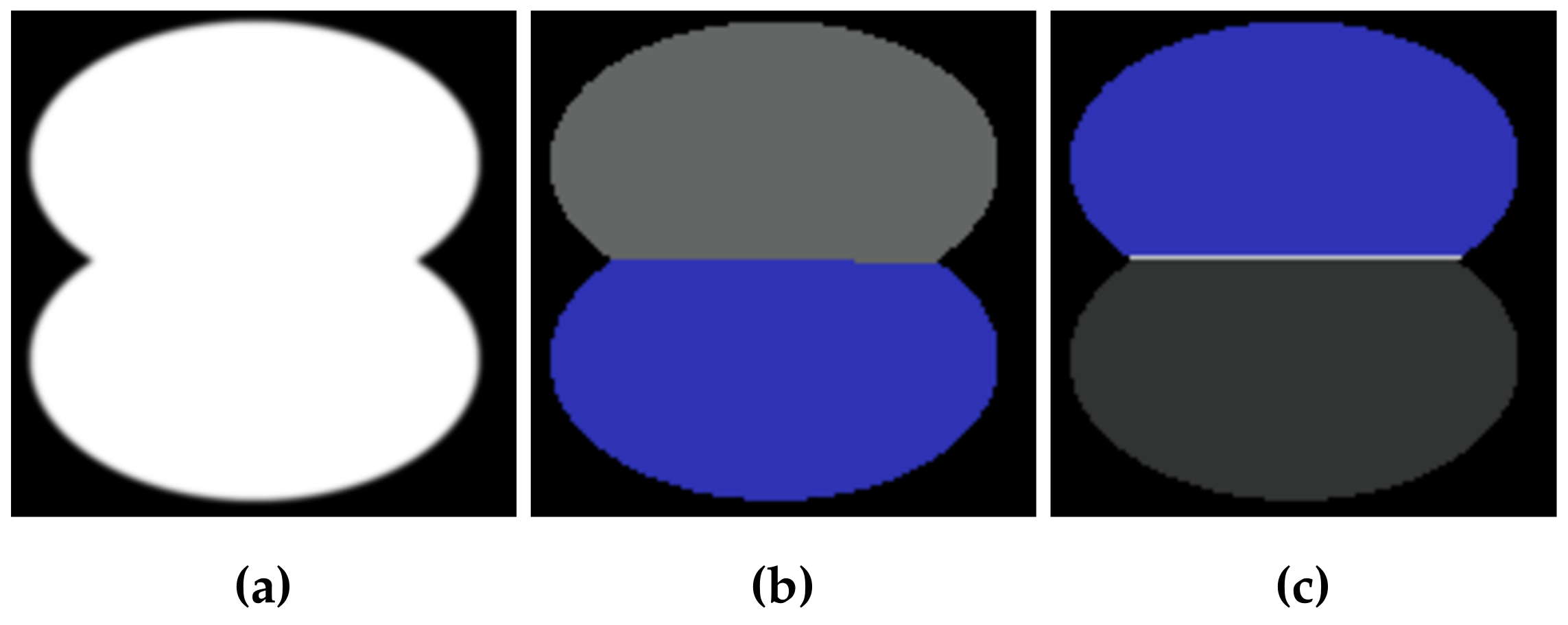
Figure 1. Difference in segmentation: (a) initial image; (b) segmentation result without watershed lines; (c) segmentation result with watershed lines.
Jimaging 04 00123 g001
Figure 2. Example of oversegmentation: (a) image; (b) segments.
Jimaging 04 00123 g002
Figure 3. Example of segmentation: (a) natural image by OpenCV; (b) natural image by Skimage; (c) contiguous objects with a similar size by OpenCV; (d) contiguous objects with a similar size by Skimage.
Jimaging 04 00123 g003
Figure 4. Image samples: (a) board; (b) cells; (c) coins; (d) fruits; (e) maze; (f) balls.
Jimaging 04 00123 g004
Figure 5. Segmentation result: (a) board; (b) cells; (c) coins; (d) fruits; (e) maze; (f) balls.
Jimaging 04 00123 g005
Figure 6. Performance measurement results without watershed lines (WL): (a) board; (b) cells; (c) coins; (d) fruits; (e) maze; (f) balls.
Jimaging 04 00123 g006
Figure 7. Performance measurement results with WL: (a) board; (b) cells; (c) coins; (d) fruits; (e) maze; (f) balls.
Jimaging 04 00123 g007
Figure 8. Memory measurement results with WL: (a) board; (b) cells; (c) coins; (d) fruits; (e) maze; (f) balls.
Jimaging 04 00123 g008
Figure 9. Memory measurement results with WL: (a) board; (b) cells; (c) coins; (d) fruits; (e) maze; (f) balls.
Jimaging 04 00123 g009
Table 1. Used watershed implementations. ITK, Insight Segmentation and Registration Toolkit; Mamba, Mathematical Morphology Image Library; Skimage, scikit-image; SMIL, Simple Morphological Image Library.
LibraryVersionSource Code LanguagePython Object
ITK4.13.0C++MorphologicalWatershedFromMarkersImageFilter
OpenCV3.4.1C++watershed
Mahotas1.4.4C++cwatershed
Mamba2.0.2CbasinSegment, watershedSegment
Skimage0.14Cythonmorphology.watershed
SMIL0.9C++basins, watershed
Table 2. Average processing time without WL (ns/element).
LibraryImage
2D3D
BoardCellsCoinsFruitsMazeAvg.Balls
ITK201246210214193213630
Mahotas165237192194161190298
Mamba4911575754071160
Skimage271466305312252321499
SMIL102163140141116132245
Table 3. Average processing time with WL (ns/element).
LibraryImage
2D3D
BoardCellsCoinsFruitsMazeAvg.Balls
ITK3063803283322923281053
Mahotas167249195202163195290
Mamba6414194945790207
Skimage1225274012511326143915968392
SMIL112182127132140139250
OpenCV365034383138