On the Application LBP Texture Descriptors and Its Variants for No-Reference Image Quality Assessment

 ,
,
Abstract
1. Introduction
2. Texture Descriptors
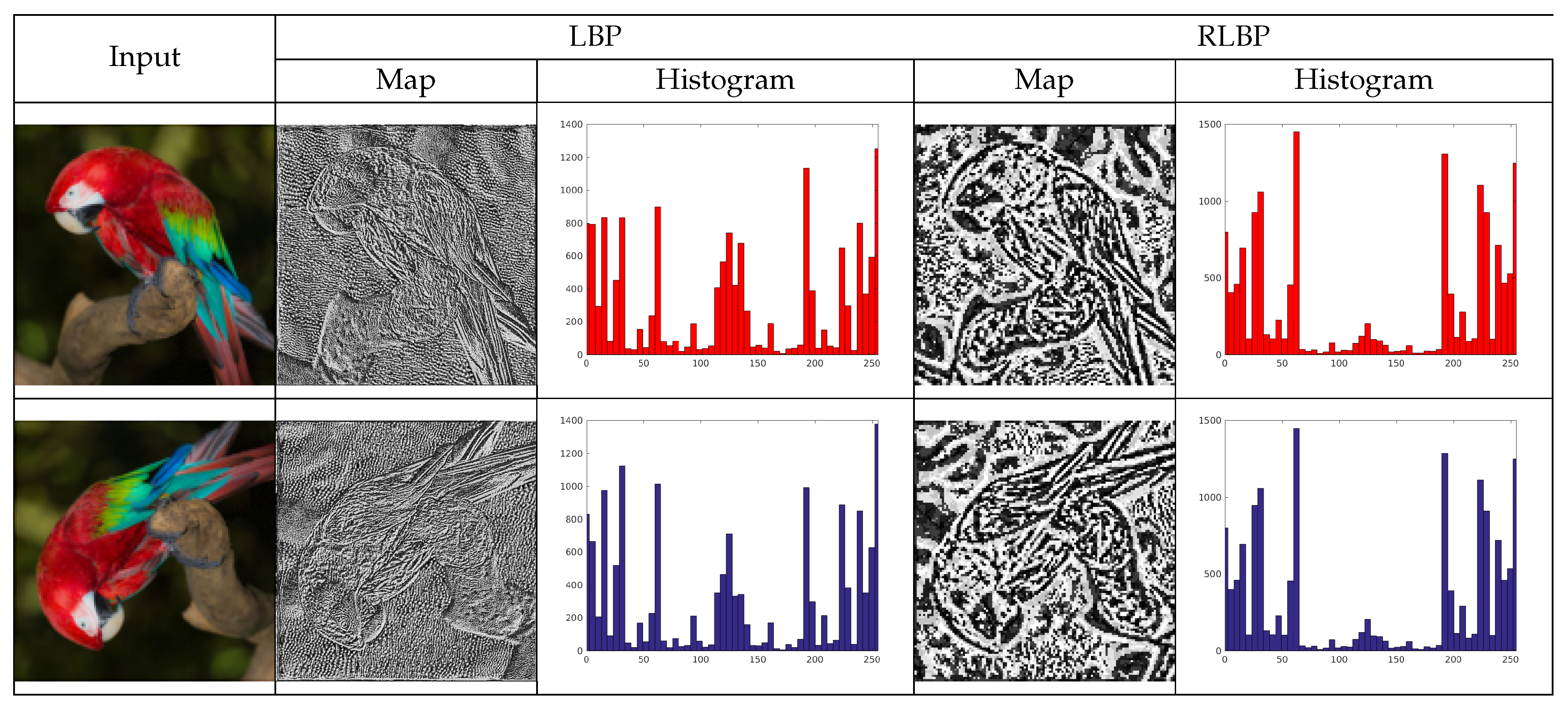
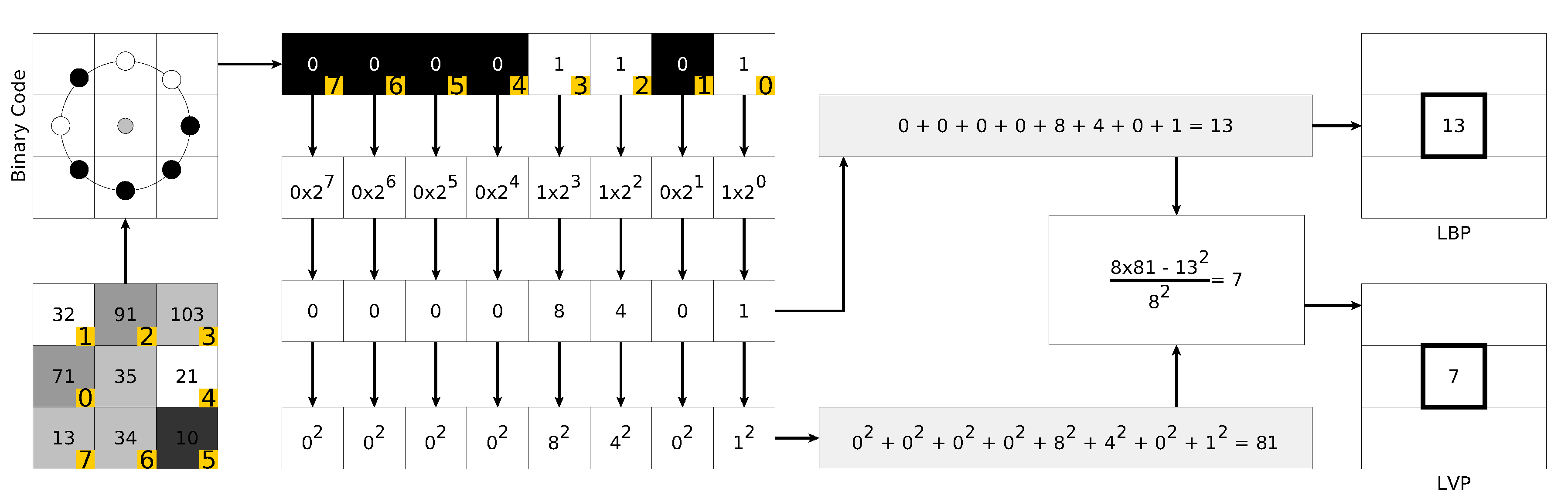
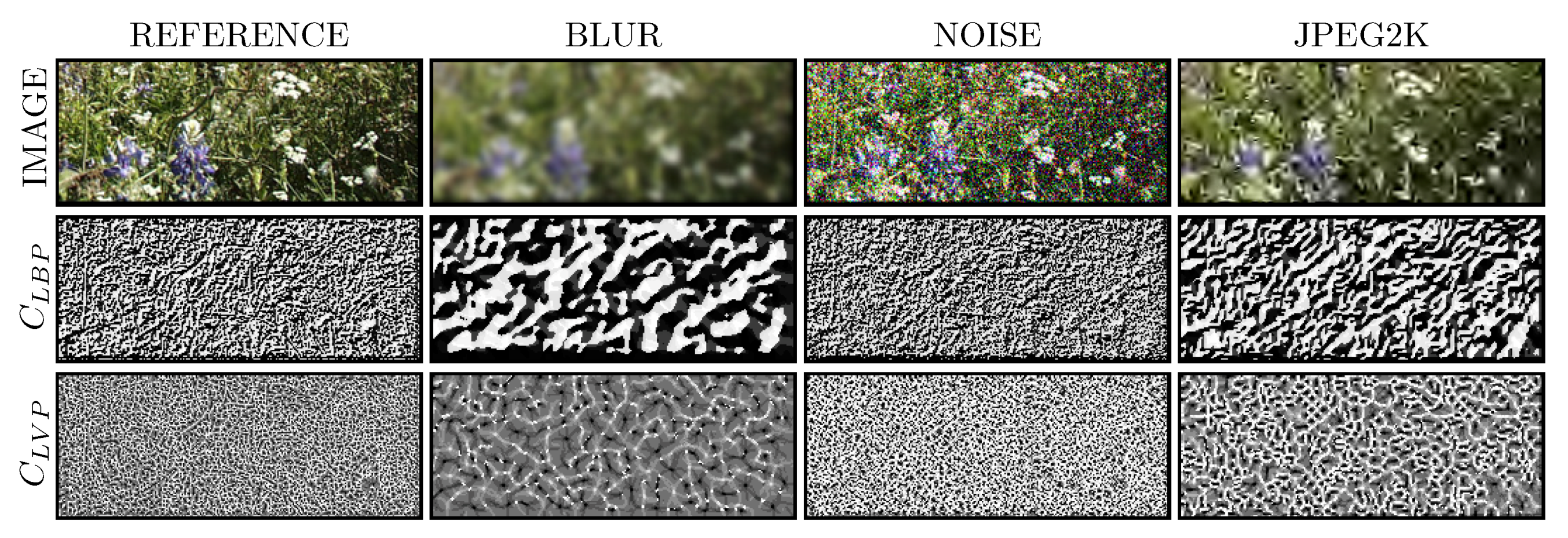
2.1. Basic Local Binary Patterns (LBP)
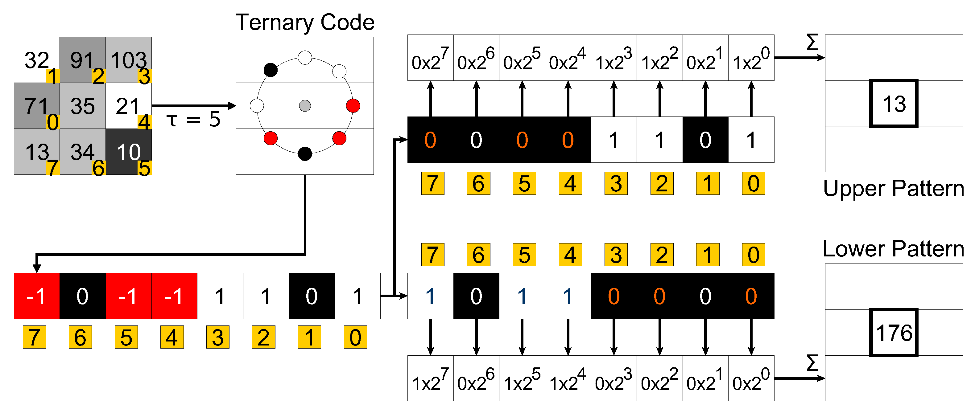
2.2. Local Ternary Patterns (LTP)
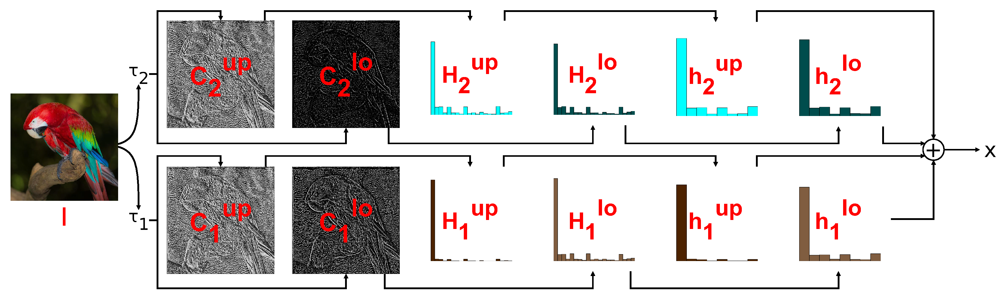
2.3. Local Phase Quantization (LPQ)
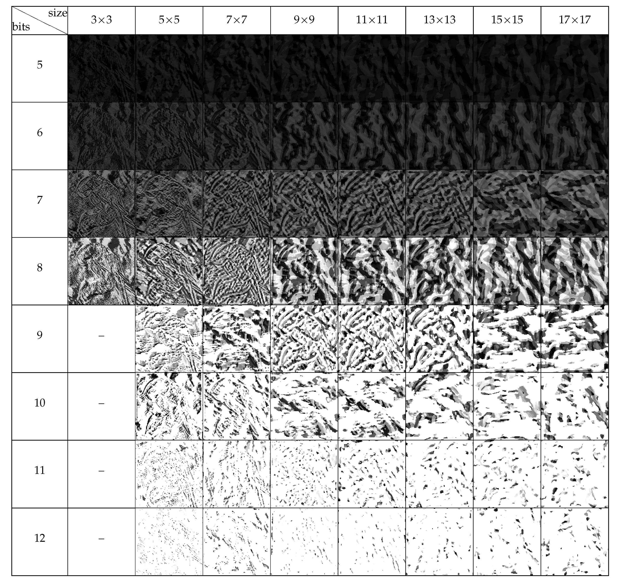
2.4. Binarized Statistical Image Features (BSIF)
2.5. Rotated Local Binary Patterns (RLBP)
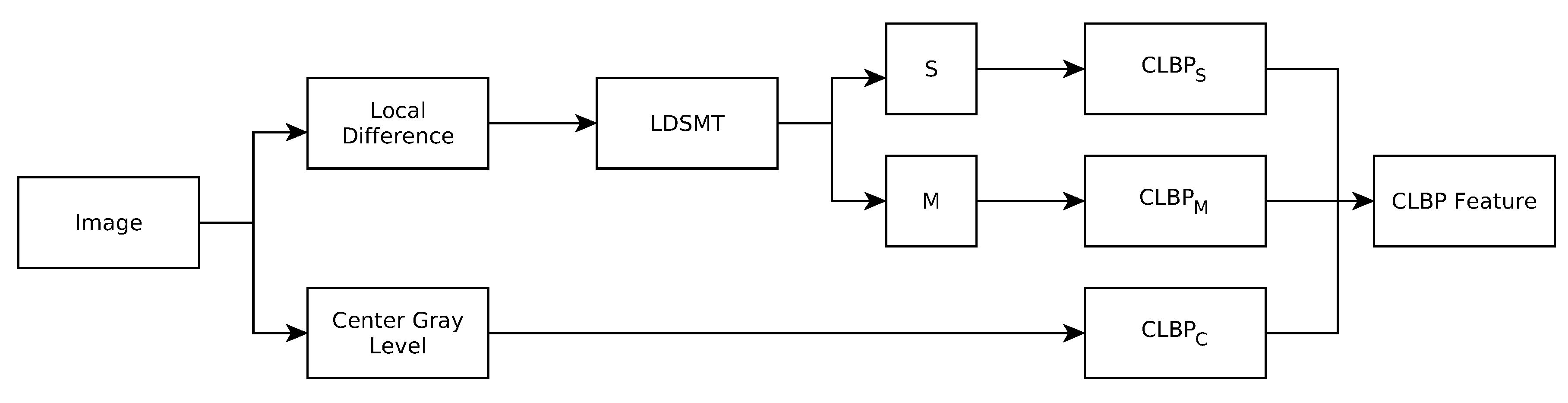
2.6. Complete Local Binary Patterns (CLBP)
2.7. Local Configuration Patterns (LCP)
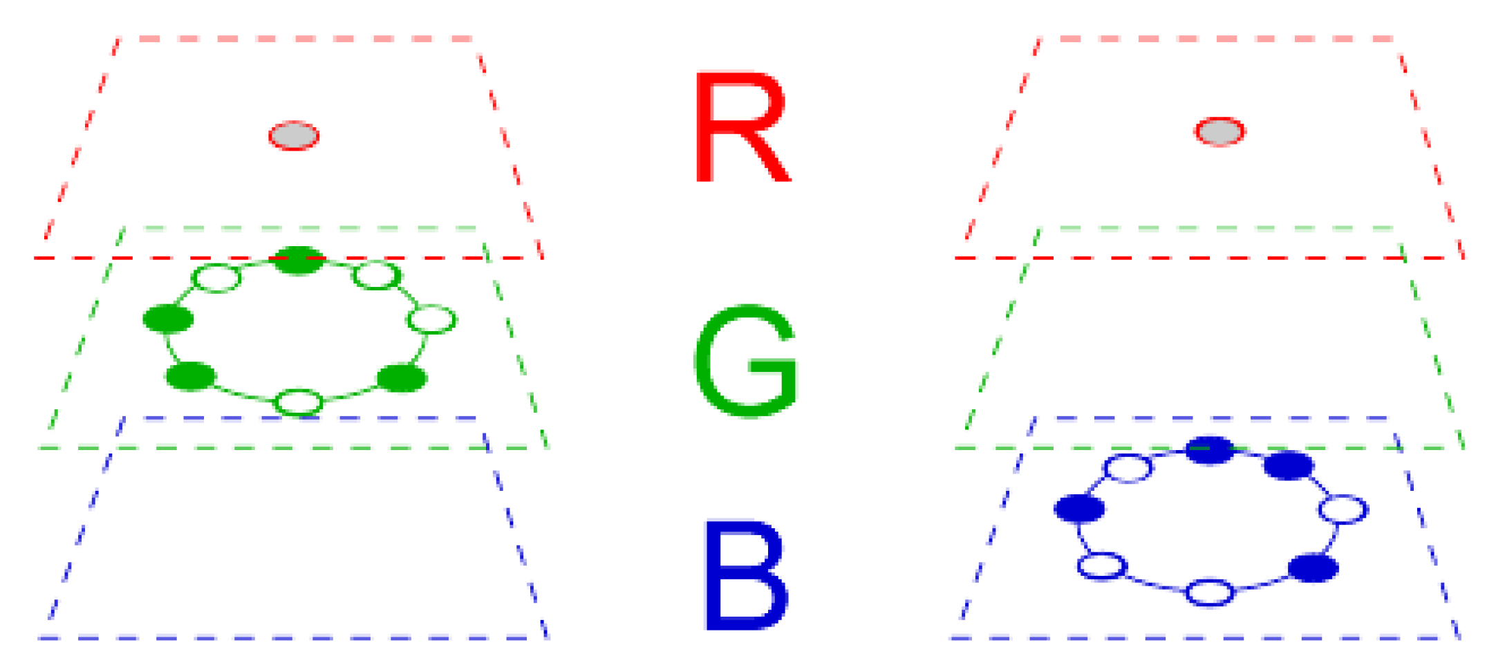
2.8. Opposite Color Local Binary Patterns (OCLBP)
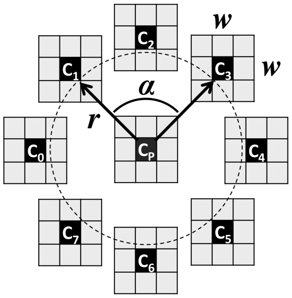
2.9. Three-Patch Local Binary Patterns (TPLBP)
2.10. Four-Patch Local Binary Patterns (FPLBP)
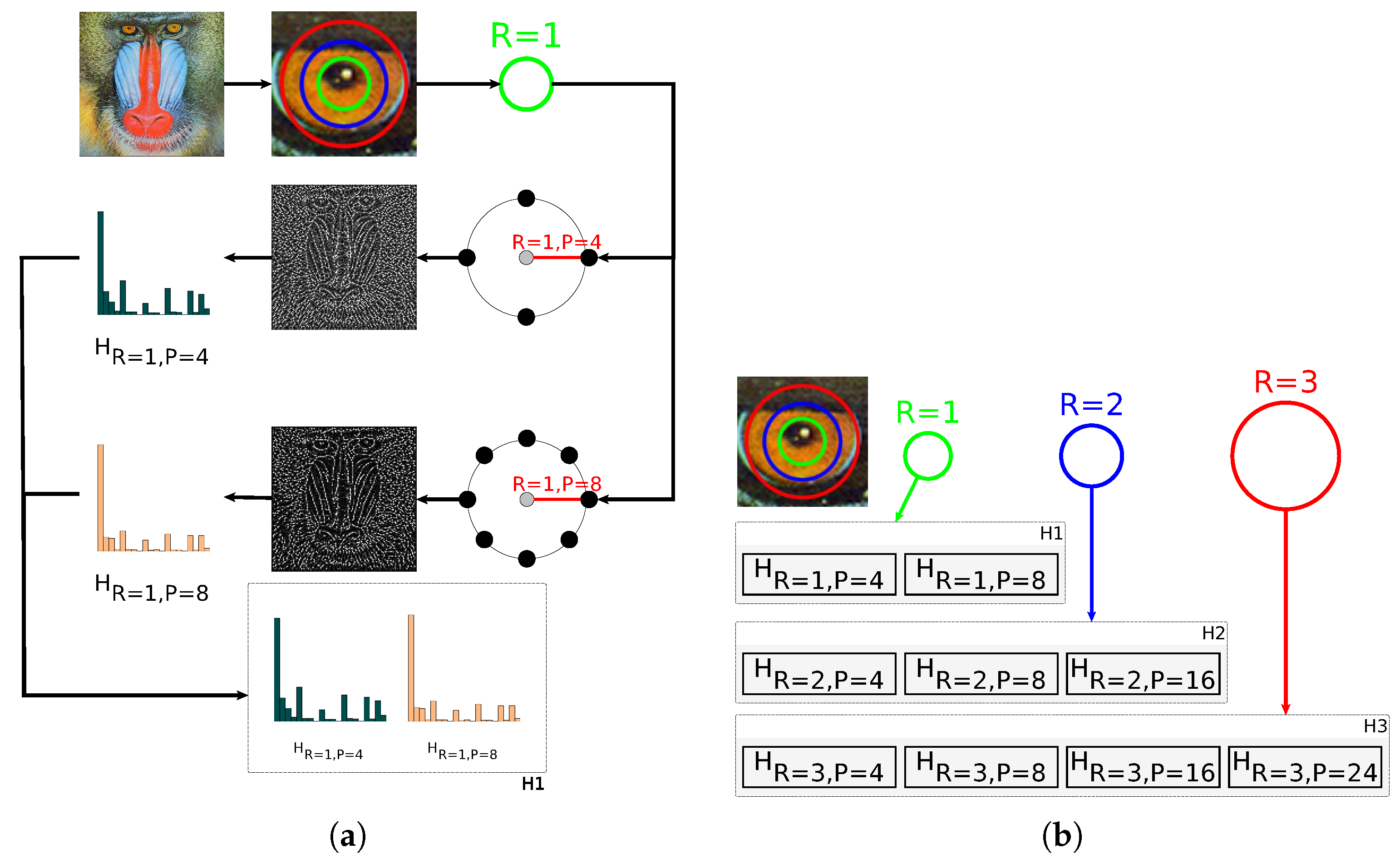
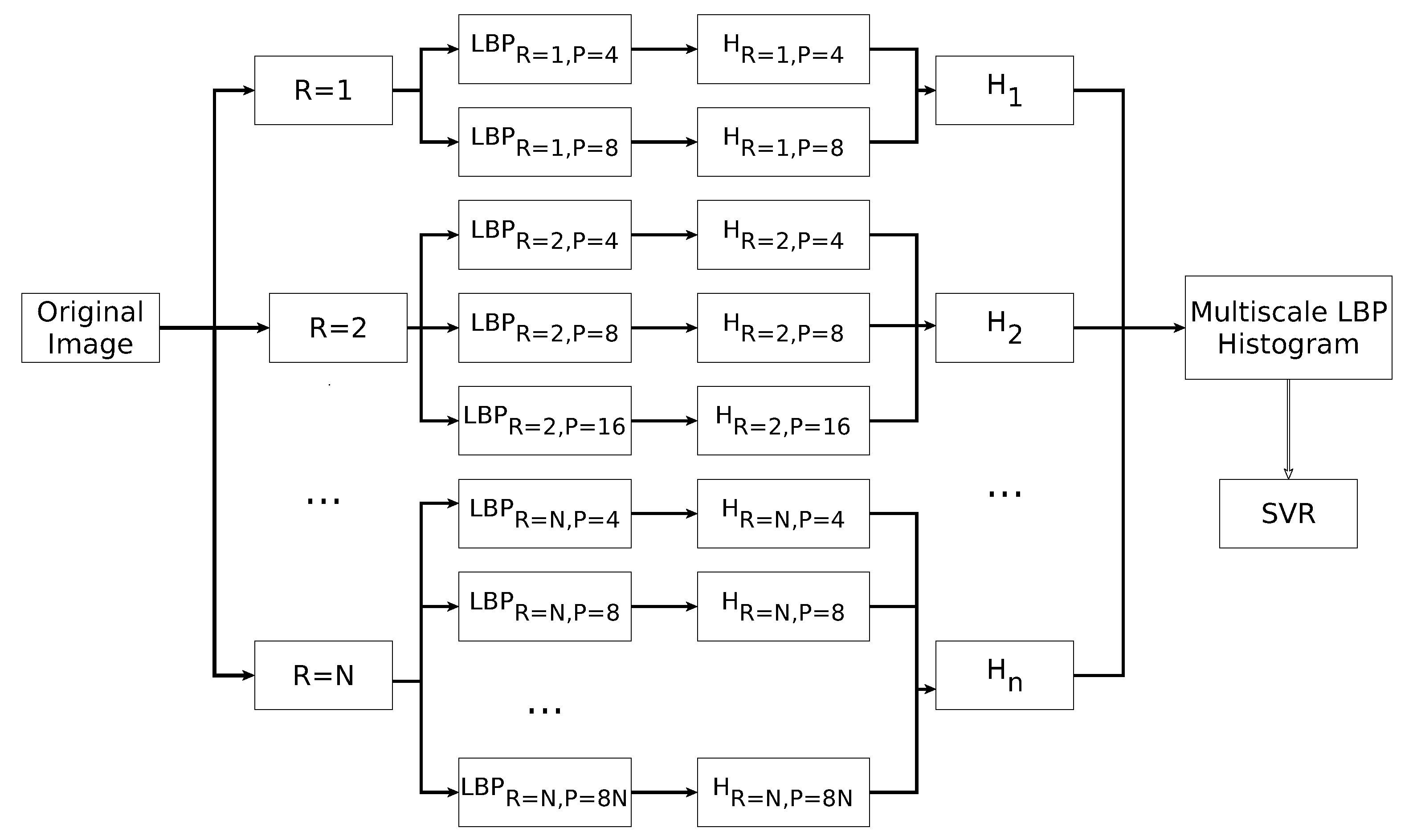
2.11. Multiscale Local Binary Patterns (MLBP)
2.12. Multiscale Local Ternary Patterns (MLTP)
2.13. Local Variance Patterns (LVP)
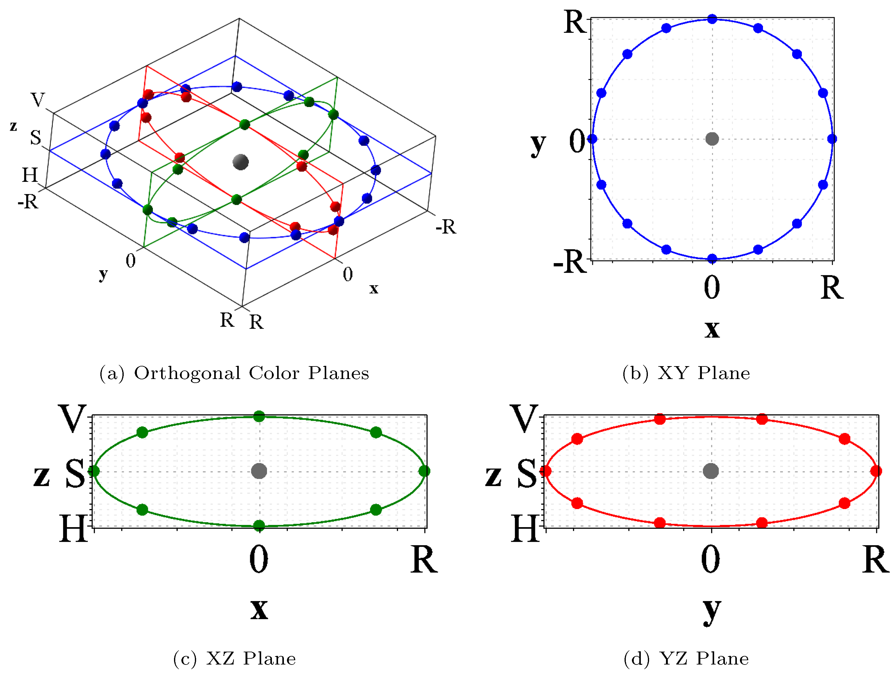
2.14. Orthogonal Color Planes Patterns (OCPP)
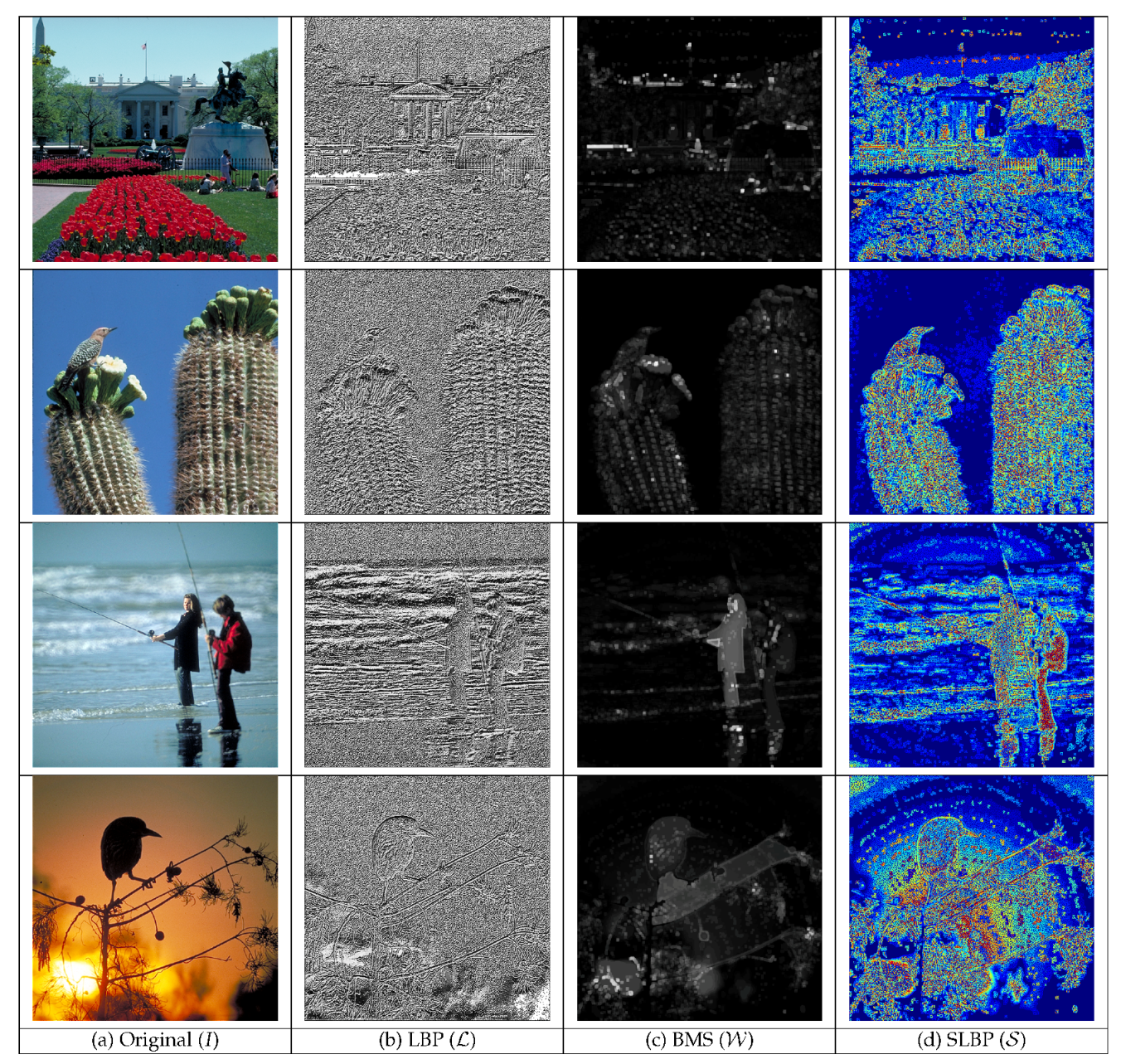
2.15. Salient Local Binary Patterns (SLBP)
2.16. Multiscale Salient Local Binary Patterns (MSLBP)
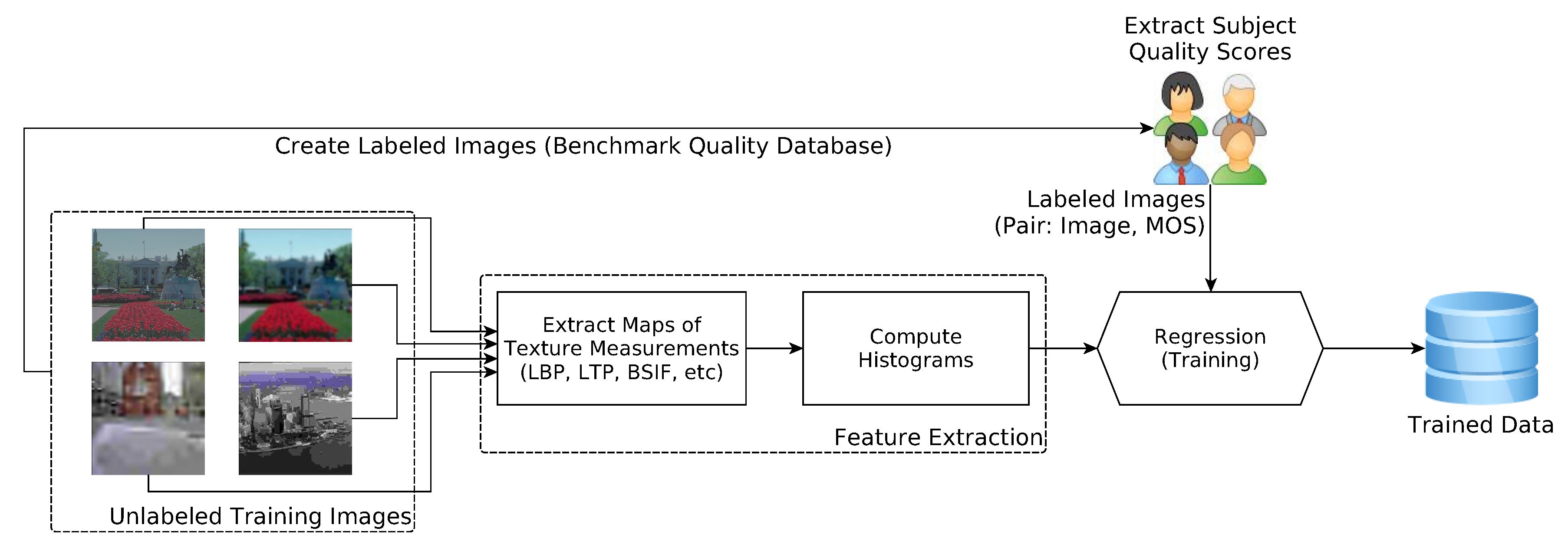
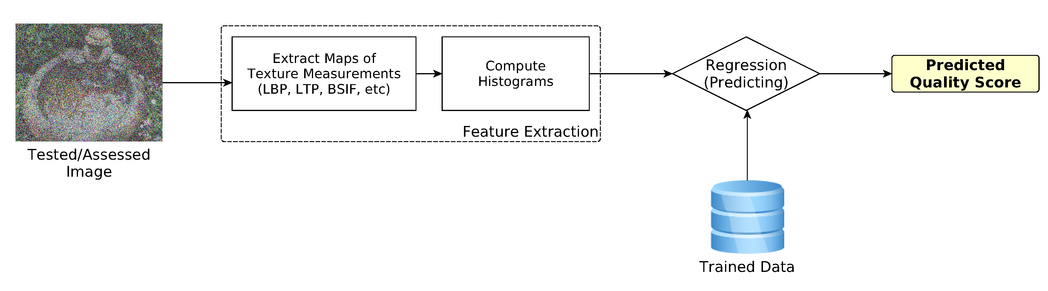
3. No-Reference Image Quality Assessment Using Texture Descriptors
3.1. Training and Testing Stages
3.2. Test Setup
- LIVE2 [100] database has 982 test images, including 29 originals. This database includes 5 categories of distortions: JPEG, JPEG 2000 (JPEG2k), white noise (WN), Gaussian blur (GB), fast fading (FF).
- CSIQ [101] database has a total fo 866 test images, consisting of 30 originals and 6 different categories of distortions. The distortions include JPEG, JPEG 2000 (JPEG2k), JPEG, white noise (WN), Gaussian blur (GB), fast fading (FF), global contrast decrements (CD), and additive Gaussian pink noise (PN).
- TID2013 [102] database contains 25 reference images with the following distortions: Additive Gaussian noise (AGN), Additive noise in color components (AGC), Spatially correlated noise (SCN), Masked noise (MN), High frequency noise (HFN), Impulse noise (IN), Quantization noise (QN), Gaussian blur (GB), Image denoising (ID), JPEG, JPEG2k, JPEG transmission errors (JPEGTE), JPEG2k transmission errors (JPEG2kTE), Non eccentricity pattern noise (NEPN), Local block-wise distortions (LBD), Intensity shift (IS), Contrast change (CC), Change of color saturation (CCS), Multiplicative Gaussian noise (MGN), Comfort noise (CN), Lossy compression (LC), Image color quantization with dither (ICQ), Chromatic aberration (CA), and Sparse sampling and reconstruction (SSR).
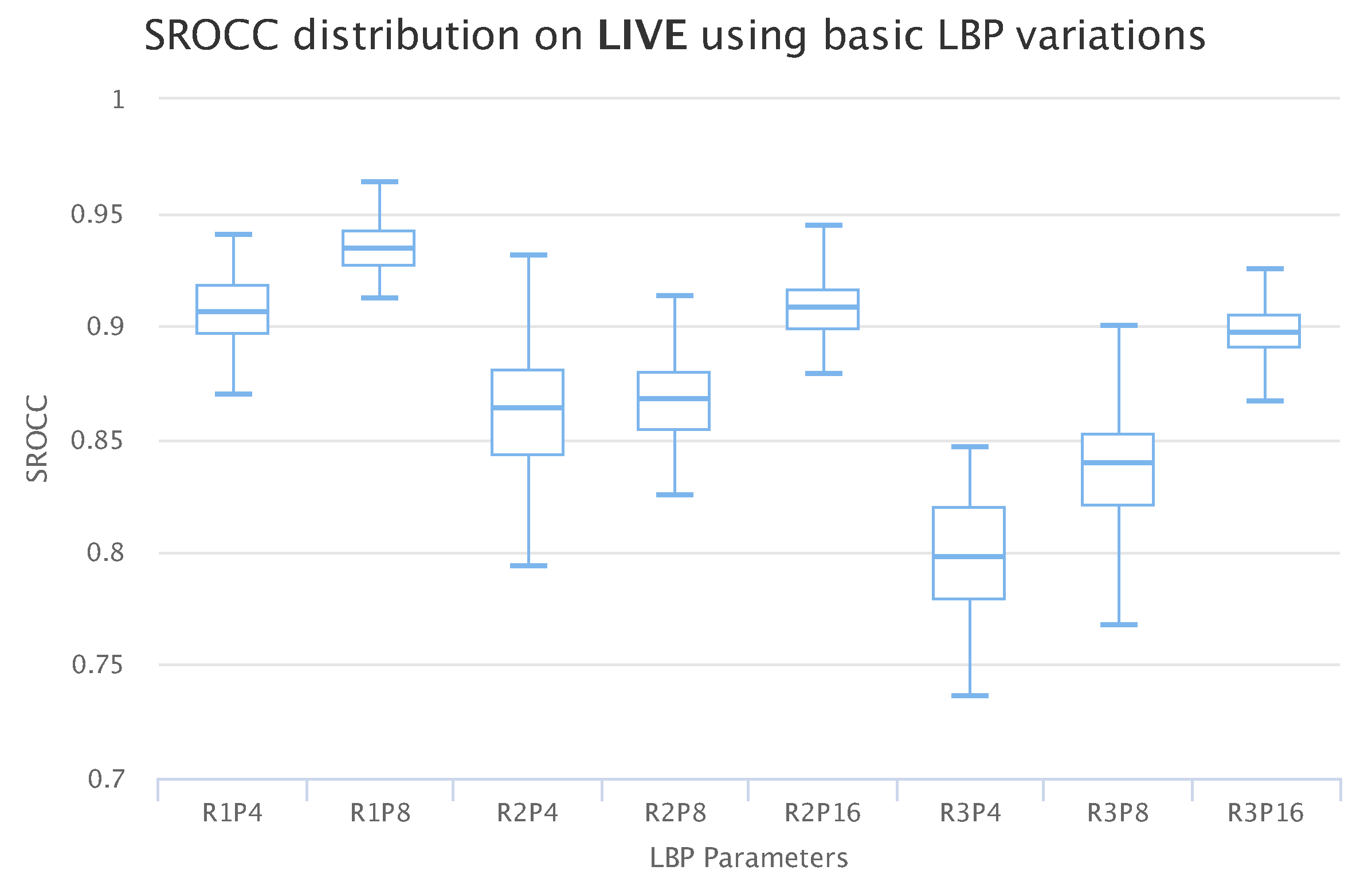
3.3. Results for Basic Descriptor with Varying Parameters
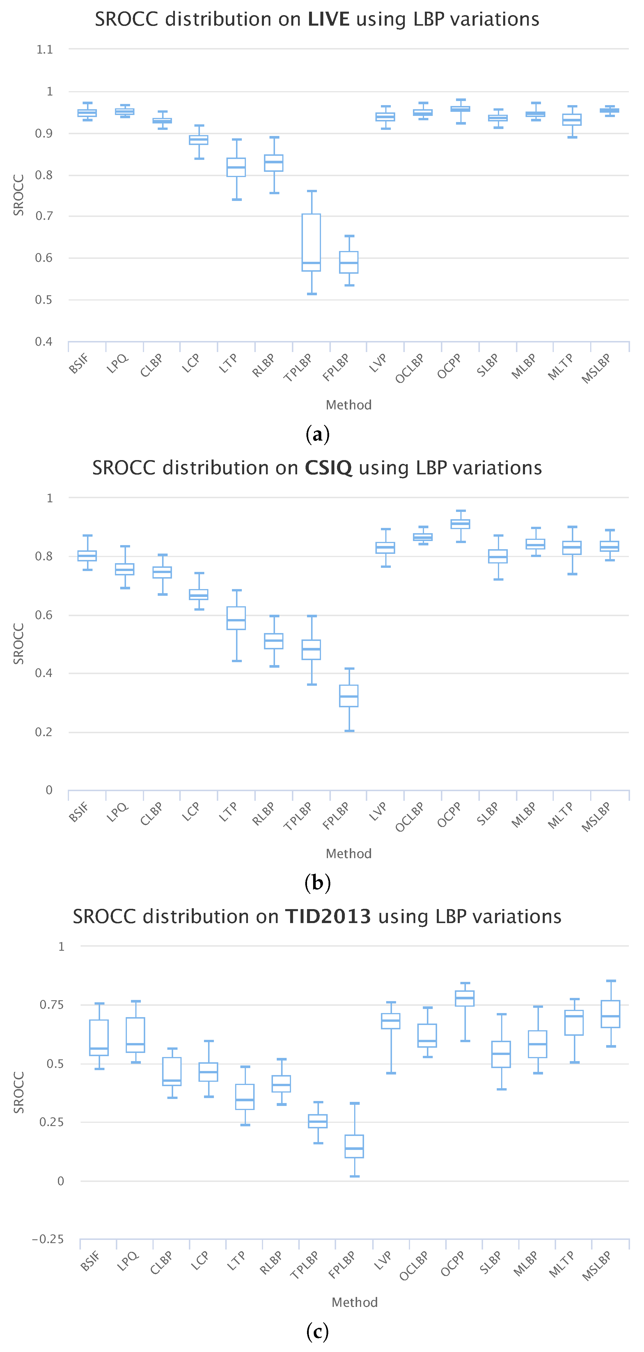
3.4. Results for Variants of Basic Descriptors
- C1: Short-term Fourier transform (STFT) with uniform window (basic version of LPQ);
- C2: STFT with Gaussian window;
- C3: Gaussian derivative quadrature filter pair;
- C4: STFT with uniform window + STFT with Gaussian window (concatenation of feature vectors produced by C1 and C2);
- C5: STFT with uniform window + STFT with Gaussian derivative quadrature filter pair (concatenation of feature vectors produced by C1 and C3);
- C6: STFT with Gaussian window + Gaussian derivative quadrature filter pair (concatenation of feature vectors produced by C2 and C3);
- C7: Concatenation of feature vectors produced by C1, C2, and C3.
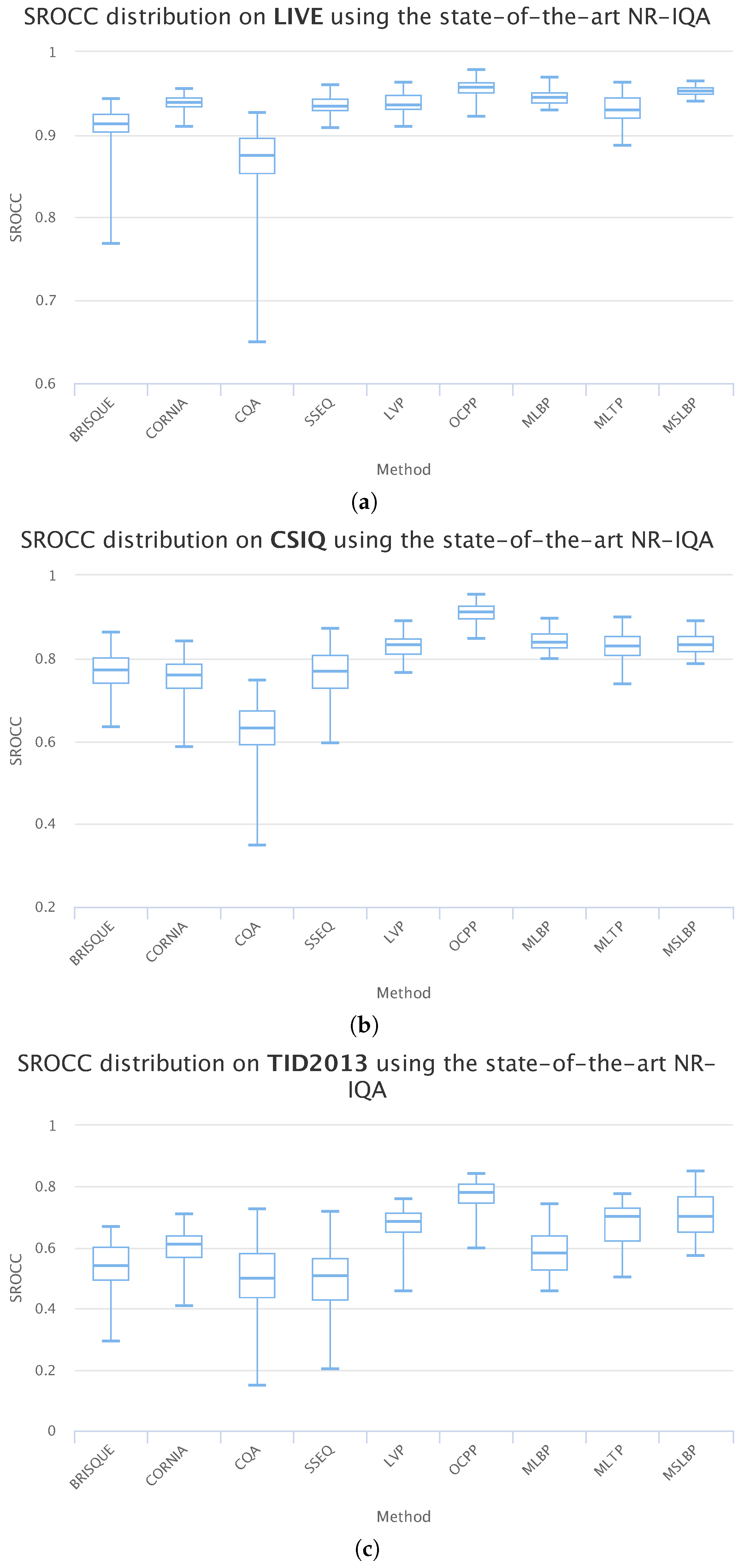
3.5. Comparison with Other IQA Methods
3.6. Prediction Performance on Cross-Database Validation
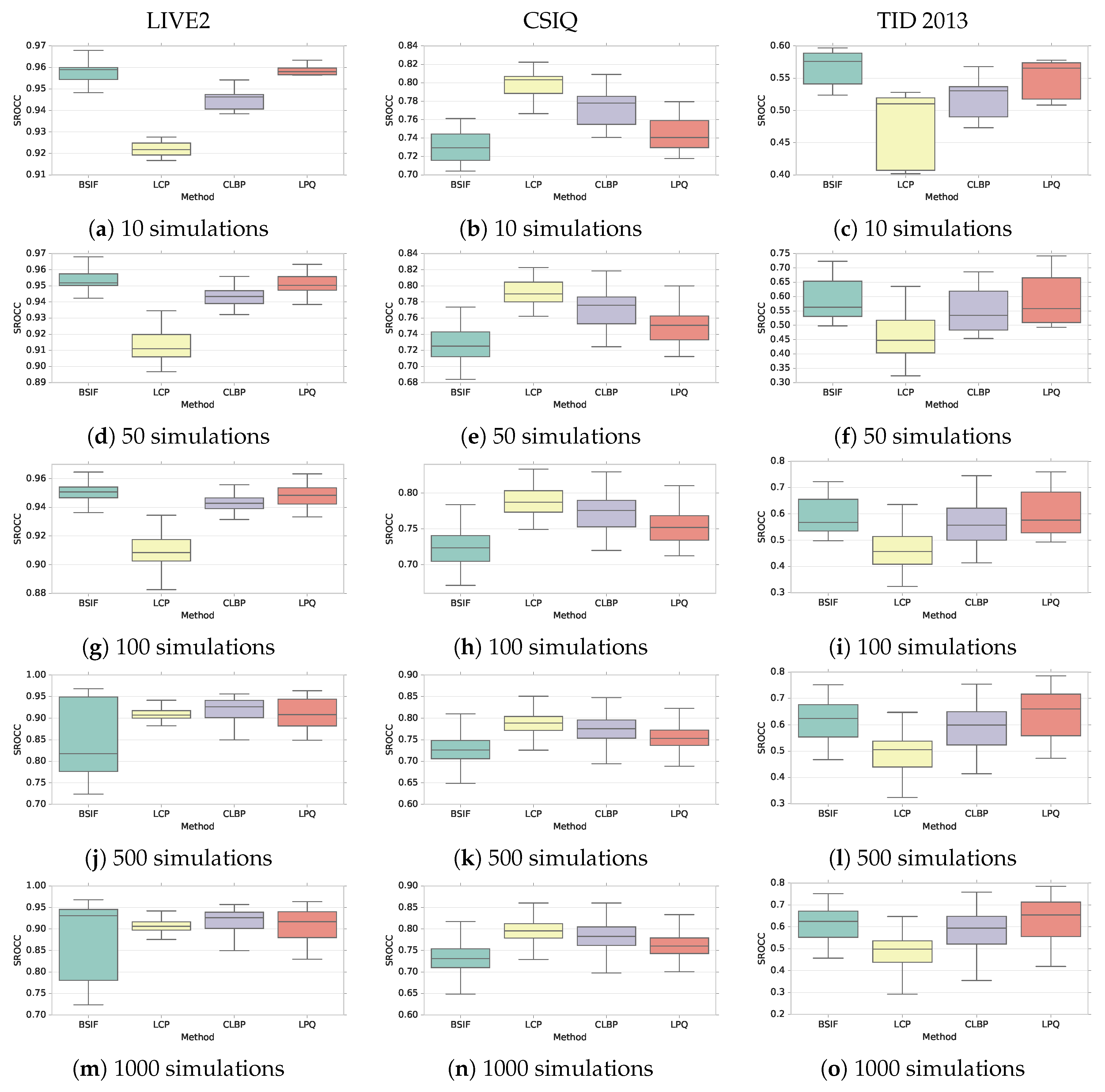
3.7. Simulation Statistics
4. Conclusions
Author Contributions
Funding
Acknowledgments
Conflicts of Interest
References
- Chen, Q.H.; Xie, X.F.; Cao, J.; Cui, X.C. Research of ROI image compression based on visual attention model. In Proceedings of the International Conference on Image Processing and Pattern Recognition in Industrial Engineering, Xi’an, China, 7–8 August 2010; Volume 7820, p. 78202W. [Google Scholar]
- Wang, Z.; Li, Q.; Shang, X. Perceptual image coding based on a maximum of minimal structural similarity criterion. In Proceedings of the IEEE International Conference on Image Processing, ICIP 2007, San Antonio, TX, USA, 16–19 September 2007; Volume 2, p. II-121. [Google Scholar]
- Chen, Z.; Guillemot, C. Perceptually-friendly H. 264/AVC video coding based on foveated just-noticeable-distortion model. IEEE Trans. Circuits Syst. Video Technol. 2010, 20, 806–819. [Google Scholar] [CrossRef]
- Ou, T.S.; Huang, Y.H.; Chen, H.H. SSIM-based perceptual rate control for video coding. IEEE Trans. Circuits Syst. Video Technol. 2011, 21, 682–691. [Google Scholar]
- Wang, Z.; Baroud, Y.; Najmabadi, S.M.; Simon, S. Low complexity perceptual image coding by just-noticeable difference model based adaptive downsampling. In Proceedings of the Picture Coding Symposium (PCS), Nuremberg, Germany, 4–7 December 2016; pp. 1–5. [Google Scholar]
- Wu, H.R.; Rao, K.R. Digital Video Image Quality and Perceptual Coding; CRC Press: Boca Raton, FL, USA, 2017. [Google Scholar]
- Zhang, F.; Liu, W.; Lin, W.; Ngan, K.N. Spread spectrum image watermarking based on perceptual quality metric. IEEE Trans. Image Process. 2011, 20, 3207–3218. [Google Scholar] [CrossRef] [PubMed]
- Urvoy, M.; Goudia, D.; Autrusseau, F. Perceptual DFT watermarking with improved detection and robustness to geometrical distortions. IEEE Trans. Inf. Forensics Secur. 2014, 9, 1108–1119. [Google Scholar] [CrossRef]
- Conviva. Viewer Experience Report. 2015. Available online: http://www.conviva.com/convivaviewer-experience-report/vxr-2015/ (accessed on 19 July 2017).
- Kupyn, O.; Budzan, V.; Mykhailych, M.; Mishkin, D.; Matas, J. DeblurGAN: Blind Motion Deblurring Using Conditional Adversarial Networks. arXiv, 2017; arXiv:1711.07064. [Google Scholar]
- Dodge, S.; Karam, L. Understanding how image quality affects deep neural networks. In Proceedings of the 2016 IEEE Eighth International Conference on Quality of Multimedia Experience (QoMEX), Lisbon, Portugal, 6–8 June 2016; pp. 1–6. [Google Scholar]
- Bhogal, A.P.S.; Söllinger, D.; Trung, P.; Hämmerle-Uhl, J.; Uhl, A. Non-reference Image Quality Assessment for Fingervein Presentation Attack Detection. In Proceedings of the Scandinavian Conference on Image Analysis, Tromsø, Norway, 12–14 June 2017; pp. 184–196. [Google Scholar]
- Söllinger, D.; Trung, P.; Uhl, A. Non-reference image quality assessment and natural scene statistics to counter biometric sensor spoofing. IET Biom. 2018, 7, 314–324. [Google Scholar] [CrossRef]
- Karahan, S.; Yildirum, M.K.; Kirtac, K.; Rende, F.S.; Butun, G.; Ekenel, H.K. How image degradations affect deep CNN-based face recognition? In Proceedings of the 2016 International Conference of the Biometrics Special Interest Group (BIOSIG), Darmstadt, Germany, 21–23 September 2016; pp. 1–5. [Google Scholar]
- Chernov, T.S.; Razumnuy, N.P.; Kozharinov, A.S.; Nikolaev, D.P.; Arlazarov, V.V. Image quality assessment for video stream recognition systems. In Proceedings of the Tenth International Conference on Machine Vision (ICMV 2017), Vienna, Austria, 13–15 November 2017; Volume 10696, p. 106961U. [Google Scholar]
- Jeelani, H.; Martin, J.; Vasquez, F.; Salerno, M.; Weller, D.S. Image quality affects deep learning reconstruction of MRI. In Proceedings of the 2018 IEEE 15th International Symposium on Biomedical Imaging (ISBI 2018), Washington, DC, USA, 4–7 April 2018; pp. 357–360. [Google Scholar]
- Choi, J.H.; Cheon, M.; Lee, J.S. Influence of Video Quality on Multi-view Activity Recognition. In Proceedings of the 2017 IEEE International Symposium on Multimedia (ISM), Taichung, Taiwan, 11–13 December 2017; pp. 511–515. [Google Scholar]
- Redmon, J.; Divvala, S.K.; Girshick, R.B.; Farhadi, A. You Only Look Once: Unified, Real-Time Object Detection. In Proceedings of the 2016 IEEE Conference on Computer Vision and Pattern Recognition, CVPR 2016, Las Vegas, NV, USA, 27–30 June 2016; pp. 779–788. [Google Scholar]
- Nah, S.; Kim, T.H.; Lee, K.M. Deep Multi-scale Convolutional Neural Network for Dynamic Scene Deblurring. In Proceedings of the 2017 IEEE Conference on Computer Vision and Pattern Recognition, CVPR 2017, Honolulu, HI, USA, 21–26 July 2017; pp. 257–265. [Google Scholar]
- Seshadrinathan, K.; Bovik, A.C. Automatic prediction of perceptual quality of multimedia signals—A survey. Multimed. Tools Appl. 2011, 51, 163–186. [Google Scholar] [CrossRef]
- Ferzli, R.; Karam, L.J. A no-reference objective image sharpness metric based on the notion of just noticeable blur (JNB). IEEE Trans. Image Process. 2009, 18, 717–728. [Google Scholar] [CrossRef] [PubMed]
- Maheshwary, P.; Shirvaikar, M.; Grecos, C. Blind image sharpness metric based on edge and texture features. In Proceedings of the Real-Time Image and Video Processing 2018, Orlando, FL, USA, 15–19 April 2018; Volume 10670, p. 1067004. [Google Scholar]
- Li, L.; Xia, W.; Lin, W.; Fang, Y.; Wang, S. No-reference and robust image sharpness evaluation based on multiscale spatial and spectral features. IEEE Trans. Multimed. 2017, 19, 1030–1040. [Google Scholar] [CrossRef]
- Ong, E.; Lin, W.; Lu, Z.; Yao, S.; Yang, X.; Jiang, L. No-reference JPEG-2000 image quality metric. In Proceedings of the 2003 International Conference on Multimedia and Expo, ICME’03, Baltimore, MD, USA, 6–9 July 2003; Volume 1, pp. I–545. [Google Scholar]
- Barland, R.; Saadane, A. Reference free quality metric for JPEG-2000 compressed images. In Proceedings of the Eighth International Symposium on Signal Processing and Its Applications, Sydney, Australia, 28–31 August 2005; Volume 1, pp. 351–354. [Google Scholar]
- Li, L.; Zhou, Y.; Lin, W.; Wu, J.; Zhang, X.; Chen, B. No-reference quality assessment of deblocked images. Neurocomputing 2016, 177, 572–584. [Google Scholar] [CrossRef]
- Gu, K.; Lin, W.; Zhai, G.; Yang, X.; Zhang, W.; Chen, C.W. No-Reference Quality Metric of Contrast-Distorted Images Based on Information Maximization. IEEE Trans. Cybern. 2017, 47, 4559–4565. [Google Scholar] [CrossRef] [PubMed]
- Gu, K.; Zhai, G.; Yang, X.; Zhang, W.; Chen, C.W. Automatic contrast enhancement technology with saliency preservation. IEEE Trans. Circuits Syst. Video Technol. 2015, 25, 1480–1494. [Google Scholar]
- Chandler, D.M. Seven challenges in image quality assessment: Past, present, and future research. ISRN Signal Process. 2013, 2013, 905685. [Google Scholar] [CrossRef]
- Chandler, D.M.; Alam, M.M.; Phan, T.D. Seven challenges for image quality research. In Proceedings of the IS&T/SPIE Electronic Imaging, San Francisco, CA, USA, 2–6 February 2014; p. 901402. [Google Scholar]
- Hemami, S.S.; Reibman, A.R. No-reference image and video quality estimation: Applications and human-motivated design. Signal Process. Image Commun. 2010, 25, 469–481. [Google Scholar] [CrossRef]
- Cheng, G.; Huang, J.; Liu, Z.; Lizhi, C. Image quality assessment using natural image statistics in gradient domain. AEU Int. J. Electron. Commun. 2011, 65, 392–397. [Google Scholar] [CrossRef]
- Appina, B.; Khan, S.; Channappayya, S.S. No-reference Stereoscopic Image Quality Assessment Using Natural Scene Statistics. Signal Process. Image Commun. 2016, 43, 1–14. [Google Scholar] [CrossRef]
- Zhang, Y.; Wu, J.; Xie, X.; Li, L.; Shi, G. Blind image quality assessment with improved natural scene statistics model. Digit. Signal Process. 2016, 57, 56–65. [Google Scholar] [CrossRef]
- Fang, Y.; Ma, K.; Wang, Z.; Lin, W.; Fang, Z.; Zhai, G. No-reference quality assessment of contrast-distorted images based on natural scene statistics. IEEE Signal Process. Lett. 2015, 22, 838–842. [Google Scholar] [CrossRef]
- Saad, M.; Bovik, A.C.; Charrier, C. A DCT statistics-based blind image quality index. IEEE Signal Process. Lett. 2010, 17, 583–586. [Google Scholar] [CrossRef]
- Ma, L.; Li, S.; Ngan, K.N. Reduced-reference image quality assessment in reorganized DCT domain. Signal Process. Image Commun. 2013, 28, 884–902. [Google Scholar] [CrossRef]
- Saad, M.A.; Bovik, A.C.; Charrier, C. Blind image quality assessment: A natural scene statistics approach in the DCT domain. IEEE Trans. Image Process. 2012, 21, 3339–3352. [Google Scholar] [CrossRef] [PubMed]
- Moorthy, A.K.; Bovik, A.C. A two-step framework for constructing blind image quality indices. IEEE Signal Process. Lett. 2010, 17, 513–516. [Google Scholar] [CrossRef]
- Moorthy, A.K.; Bovik, A.C. Blind image quality assessment: From natural scene statistics to perceptual quality. IEEE Trans. Image Process. 2011, 20, 3350–3364. [Google Scholar] [CrossRef] [PubMed]
- He, L.; Tao, D.; Li, X.; Gao, X. Sparse representation for blind image quality assessment. In Proceedings of the 2012 IEEE Conference on Computer Vision and Pattern Recognition (CVPR), Providence, RI, USA, 16–21 June 2012; pp. 1146–1153. [Google Scholar]
- Mittal, A.; Moorthy, A.K.; Bovik, A.C. No-reference image quality assessment in the spatial domain. IEEE Trans. Image Process. 2012, 21, 4695–4708. [Google Scholar] [CrossRef] [PubMed]
- Kang, L.; Ye, P.; Li, Y.; Doermann, D. Convolutional neural networks for no-reference image quality assessment. In Proceedings of the IEEE Conference on Computer Vision and Pattern Recognition, Columbus, OH, USA, 23–28 June 2014; pp. 1733–1740. [Google Scholar]
- Li, J.; Zou, L.; Yan, J.; Deng, D.; Qu, T.; Xie, G. No-reference image quality assessment using Prewitt magnitude based on convolutional neural networks. Signal Image Video Process. 2016, 10, 609–616. [Google Scholar] [CrossRef]
- Bosse, S.; Maniry, D.; Wiegand, T.; Samek, W. A deep neural network for image quality assessment. In Proceedings of the 2016 IEEE International Conference on Image Processing (ICIP), Phoenix, AZ, USA, 25–28 September 2016; pp. 3773–3777. [Google Scholar]
- Kuzovkin, I.; Vicente, R.; Petton, M.; Lachaux, J.P.; Baciu, M.; Kahane, P.; Rheims, S.; Vidal, J.R.; Aru, J. Frequency-Resolved Correlates of Visual Object Recognition in Human Brain Revealed by Deep Convolutional Neural Networks. bioRxiv 2017, 133694. [Google Scholar] [CrossRef]
- Yamins, D.L.; DiCarlo, J.J. Using goal-driven deep learning models to understand sensory cortex. Nat. Neurosci. 2016, 19, 356–365. [Google Scholar] [CrossRef] [PubMed]
- Bianco, S.; Celona, L.; Napoletano, P.; Schettini, R. On the use of deep learning for blind image quality assessment. Signal Image Video Process. 2018, 12, 355–362. [Google Scholar] [CrossRef]
- Scott, E.T.; Hemami, S.S. No-Reference Utility Estimation with a Convolutional Neural Network. Electron. Imaging 2018, 2018, 1–6. [Google Scholar] [CrossRef]
- Jia, S.; Zhang, Y. Saliency-based deep convolutional neural network for no-reference image quality assessment. Multimed. Tools Appl. 2018, 77, 14859–14872. [Google Scholar] [CrossRef]
- Zhang, L.; Shen, Y.; Li, H. VSI: A visual saliency-induced index for perceptual image quality assessment. IEEE Trans. Image Process. 2014, 23, 4270–4281. [Google Scholar] [CrossRef] [PubMed]
- Farias, M.C.; Akamine, W.Y. On performance of image quality metrics enhanced with visual attention computational models. Electron. Lett. 2012, 48, 631–633. [Google Scholar] [CrossRef]
- Engelke, U.; Kaprykowsky, H.; Zepernick, H.J.; Ndjiki-Nya, P. Visual attention in quality assessment. IEEE Signal Process. Mag. 2011, 28, 50–59. [Google Scholar] [CrossRef]
- Gu, K.; Wang, S.; Yang, H.; Lin, W.; Zhai, G.; Yang, X.; Zhang, W. Saliency-guided quality assessment of screen content images. IEEE Trans. Multimed. 2016, 18, 1098–1110. [Google Scholar] [CrossRef]
- You, J.; Perkis, A.; Hannuksela, M.M.; Gabbouj, M. Perceptual quality assessment based on visual attention analysis. In Proceedings of the 17th ACM international conference on Multimedia, Beijing, China, 19–24 October 2009; pp. 561–564. [Google Scholar]
- Le Meur, O.; Ninassi, A.; Le Callet, P.; Barba, D. Overt visual attention for free-viewing and quality assessment tasks: Impact of the regions of interest on a video quality metric. Signal Process. Image Commun. 2010, 25, 547–558. [Google Scholar] [CrossRef]
- Le Meur, O.; Ninassi, A.; Le Callet, P.; Barba, D. Do video coding impairments disturb the visual attention deployment? Signal Process. Image Commun. 2010, 25, 597–609. [Google Scholar] [CrossRef]
- Akamine, W.Y.; Farias, M.C. Video quality assessment using visual attention computational models. J. Electron. Imaging 2014, 23, 061107. [Google Scholar] [CrossRef]
- Ciocca, G.; Corchs, S.; Gasparini, F. A complexity-based image analysis to investigate interference between distortions and image contents in image quality assessment. In Proceedings of the International Workshop on Computational Color Imaging, Milan, Italy, 29–31 March 2017; pp. 105–121. [Google Scholar]
- Larson, E.C.; Chandler, D.M. Most apparent distortion: full-reference image quality assessment and the role of strategy. J. Electron. Imaging 2010, 19, 011006. [Google Scholar]
- Liu, M.; Wang, M.; Wang, J.; Li, D. Comparison of random forest, support vector machine and back propagation neural network for electronic tongue data classification: Application to the recognition of orange beverage and Chinese vinegar. Sens. Actuators B Chem. 2013, 177, 970–980. [Google Scholar] [CrossRef]
- Petrou, M.; Sevilla, P.G. Image Processing: Dealing with Texture; John Wiley and Sons: Hoboken, NJ, USA, 2006. [Google Scholar]
- Davies, E.R. Introduction to Texture Analysis. In Handbook of Texture Analysis; Mirmehdi, M., Xie, X., Suri, J., Eds.; Imperial College Press: London, UK, 2008; Chapter 1; pp. 1–31. [Google Scholar]
- Galloway, M.M. Texture analysis using gray level run lengths. Comput. Graph. Image Process. 1975, 4, 172–179. [Google Scholar] [CrossRef]
- Soh, L.K.; Tsatsoulis, C. Texture analysis of SAR sea ice imagery using gray level co-occurrence matrices. IEEE Trans. Geosci. Remote Sens. 1999, 37, 780–795. [Google Scholar] [CrossRef]
- He, D.C.; Wang, L. Texture unit, texture spectrum, and texture analysis. IEEE Trans. Geosci. Remote Sens. 1990, 28, 509–512. [Google Scholar]
- Julesz, B. Textons, the elements of texture perception, and their interactions. Nature 1981, 290, 91–97. [Google Scholar] [CrossRef] [PubMed]
- Ojala, T.; Pietikäinen, M.; Mäenpää, T. Multiresolution gray-scale and rotation invariant texture classification with local binary patterns. IEEE Trans. Pattern Anal. Mach. Intell. 2002, 24, 971–987. [Google Scholar] [CrossRef]
- Hadid, A.; Ylioinas, J.; Bengherabi, M.; Ghahramani, M.; Taleb-Ahmed, A. Gender and texture classification: A comparative analysis using 13 variants of local binary patterns. Pattern Recognit. Lett. 2015, 68, 231–238. [Google Scholar] [CrossRef]
- Brahnam, S.; Jain, L.C.; Lumini, A.; Nanni, L. Introduction to Local Binary Patterns: New Variants and Applications. In Local Binary Patterns; Studies in Computational Intelligence; Brahnam, S., Jain, L.C., Nanni, L., Lumini, A., Eds.; Springer: Berlin/Heidelberg, Germany, 2013; Volume 506, pp. 1–13. [Google Scholar]
- Pietikäinen, M.; Ojala, T.; Xu, Z. Rotation-invariant texture classification using feature distributions. Pattern Recognit. 2000, 33, 43–52. [Google Scholar] [CrossRef]
- Ojansivu, V.; Heikkilä, J. Blur insensitive texture classification using local phase quantization. In Proceedings of the International Conference on Image and Signal Processing, Cherbourg-Octeville, France, 1–3 July 2008; pp. 236–243. [Google Scholar]
- Kannala, J.; Rahtu, E. Bsif: Binarized statistical image features. In Proceedings of the 2012 21st International Conference on Pattern Recognition (ICPR), Tsukuba, Japan, 11–15 November 2012; pp. 1363–1366. [Google Scholar]
- Arashloo, S.R.; Kittler, J. Dynamic texture recognition using multiscale binarized statistical image features. IEEE Trans. Multimed. 2014, 16, 2099–2109. [Google Scholar] [CrossRef]
- Raja, K.B.; Raghavendra, R.; Busch, C. Binarized statistical features for improved iris and periocular recognition in visible spectrum. In Proceedings of the 2014 International Workshop on Biometrics and Forensics (IWBF), Valletta, Malta, 27–28 March 2014; pp. 1–6. [Google Scholar]
- Arashloo, S.R.; Kittler, J.; Christmas, W. Face spoofing detection based on multiple descriptor fusion using multiscale dynamic binarized statistical image features. IEEE Trans. Inf. Forensics Secur. 2015, 10, 2396–2407. [Google Scholar] [CrossRef]
- Raghavendra, R.; Busch, C. Robust scheme for iris presentation attack detection using multiscale binarized statistical image features. IEEE Trans. Inf. Forensics Secur. 2015, 10, 703–715. [Google Scholar] [CrossRef]
- Mehta, R.; Egiazarian, K.O. Rotated Local Binary Pattern (RLBP)-Rotation Invariant Texture Descriptor; ICPRAM: Barcelona, Spain, 2013; pp. 497–502. [Google Scholar]
- Mehta, R.; Egiazarian, K. Dominant rotated local binary patterns (DRLBP) for texture classification. Pattern Recognit. Lett. 2016, 71, 16–22. [Google Scholar] [CrossRef]
- Kullback, S.; Leibler, R.A. On information and sufficiency. Ann. Math. Stat. 1951, 22, 79–86. [Google Scholar] [CrossRef]
- Briët, J.; Harremoës, P. Properties of classical and quantum Jensen-Shannon divergence. Phys. Rev. A 2009, 79, 052311. [Google Scholar] [CrossRef]
- Ye, N.; Borror, C.M.; Parmar, D. Scalable Chi-Square Distance versus Conventional Statistical Distance for Process Monitoring with Uncorrelated Data Variables. Qual. Reliab. Eng. Int. 2003, 19, 505–515. [Google Scholar] [CrossRef]
- Guo, Z.; Zhang, L.; Zhang, D. A completed modeling of local binary pattern operator for texture classification. IEEE Trans. Image Process. 2010, 19, 1657–1663. [Google Scholar] [PubMed]
- Guo, Y.; Zhao, G.; Pietikäinen, M. Texture Classification using a Linear Configuration Model based Descriptor. In Proceedings of the British Machine Vision Conference; BMVA Press: Dundee, UK, 2011; pp. 119.1–119.10. [Google Scholar]
- Mäenpää, T. The Local Binary Pattern Approach to Texture Analysis: Extensions and Applications; Oulun Yliopisto: Oulu, Finland, 2003. [Google Scholar]
- Jain, A.; Healey, G. A multiscale representation including opponent color features for texture recognition. IEEE Trans. Image Process. 1998, 7, 124–128. [Google Scholar] [CrossRef] [PubMed]
- Wolf, L.; Hassner, T.; Taigman, Y. Descriptor Based Methods in the Wild. In Workshop on Faces in ‘Real-Life’ Images: Detection, Alignment, and Recognition; Erik Learned-Miller and Andras Ferencz and Frédéric Jurie: Marseille, France, 2008. [Google Scholar]
- Chang, D.J.; Desoky, A.H.; Ouyang, M.; Rouchka, E.C. Compute pairwise manhattan distance and pearson correlation coefficient of data points with gpu. In Proceedings of the 10th ACIS International Conference on Software Engineering, Artificial Intelligences, Networking and Parallel/Distributed Computing, Daegu, Korea, 27–29 May 2009; pp. 501–506. [Google Scholar]
- De Maesschalck, R.; Jouan-Rimbaud, D.; Massart, D.L. The mahalanobis distance. Chemom. Intell. Lab. Syst. 2000, 50, 1–18. [Google Scholar] [CrossRef]
- Merigó, J.M.; Casanovas, M. A new Minkowski distance based on induced aggregation operators. Int. J. Comput. Intell. Syst. 2011, 4, 123–133. [Google Scholar] [CrossRef]
- Freitas, P.G.; Akamine, W.Y.; Farias, M.C. Blind Image Quality Assessment Using Multiscale Local Binary Patterns. J. Imaging Sci. Technol. 2016, 60, 60405-1. [Google Scholar] [CrossRef]
- Anthimopoulos, M.; Gatos, B.; Pratikakis, I. Detection of artificial and scene text in images and video frames. Pattern Anal. Appl. 2013, 16, 431–446. [Google Scholar] [CrossRef]
- Freitas, P.G.; Akamine, W.Y.; Farias, M.C. No-reference image quality assessment based on statistics of Local Ternary Pattern. In Proceedings of the 2016 Eighth International Conference on Quality of Multimedia Experience (QoMEX), Lisbon, Portugal, 6–8 June 2016; pp. 1–6. [Google Scholar]
- Zhang, J.; Sclaroff, S. Exploiting surroundedness for saliency detection: A Boolean map approach. IEEE Trans. Pattern Anal. Mach. Intell. 2016, 38, 889–902. [Google Scholar] [CrossRef] [PubMed]
- Fernández-Delgado, M.; Cernadas, E.; Barro, S.; Amorim, D. Do we need hundreds of classifiers to solve real world classification problems? J. Mach. Learn. Res. 2014, 15, 3133–3181. [Google Scholar]
- Ye, P.; Kumar, J.; Kang, L.; Doermann, D. Unsupervised feature learning framework for no-reference image quality assessment. In Proceedings of the 2012 IEEE Conference on Computer Vision and Pattern Recognition (CVPR), Providence, RI, USA, 16–21 June 2012; pp. 1098–1105. [Google Scholar]
- Liu, L.; Dong, H.; Huang, H.; Bovik, A.C. No-reference image quality assessment in curvelet domain. Signal Process. Image Commun. 2014, 29, 494–505. [Google Scholar] [CrossRef]
- Liu, L.; Liu, B.; Huang, H.; Bovik, A.C. No-reference image quality assessment based on spatial and spectral entropies. Signal Process. Image Commun. 2014, 29, 856–863. [Google Scholar] [CrossRef]
- Pedregosa, F.; Varoquaux, G.; Gramfort, A.; Michel, V.; Thirion, B.; Grisel, O.; Blondel, M.; Prettenhofer, P.; Weiss, R.; Dubourg, V.; et al. Scikit-learn: Machine Learning in Python. J. Mach. Learn. Res. 2011, 12, 2825–2830. [Google Scholar]
- Sheikh, H.R.; Wang, Z.; Cormack, L.; Bovik, A.C. LIVE Image Quality Assessment Database Release 2. 2015. Available online: http://live.ece.utexas.edu/research/quality (accessed on 30 September 2016).
- Larson, E.C.; Chandler, D. Categorical Image Quality (CSIQ) Database. 2010. Available online: http://vision.okstate.edu/csiq (accessed on 30 September 2016).
- Ponomarenko, N.; Jin, L.; Ieremeiev, O.; Lukin, V.; Egiazarian, K.; Astola, J.; Vozel, B.; Chehdi, K.; Carli, M.; Battisti, F.; et al. Image database TID2013: Peculiarities, results and perspectives. Signal Process. Image Commun. 2015, 30, 57–77. [Google Scholar] [CrossRef]


| Abbreviation | Name | Parameters |
|---|---|---|
| LBP | Basic Local Binary Patterns with rotation invariance | Radius (R) and number of neighbors (P) |
| LBP | Uniform Local Binary Patterns | Radius (R) and number of neighbors (P) |
| LBP | Uniform Local Binary Patterns with rotation invariance | Radius (R) and number of neighbors (P) |
| BSIF | Binarized Statistical Image Features | Window size and number of bits |
| LPQ | Local Phase Quantization) | Local frequency estimation |
| CLBP | Complete Local Binary Patterns | CLBP-S, CLBP-C, and CLBP-M |
| LCP | Local Configuration Patterns | Radius (R) and number of neighbors (P) |
| LTP | Local Ternary Patterns | Threshold (), Radius (R) and number of neighbors (P) |
| RLBP | Rotated Local Binary Patterns | Radius (R) and number of neighbors (P) |
| TPLBP | Three-Patch Local Binary Patterns | Patch size (w), Radius (R), and angle between neighboring patches |
| FPLBP | Four-Patch Local Binary Patterns | Patch size (w), Radius of first ring (R1), Radius of second ring (R2), and angle between neighboring patches |
| LVP | Local Variance Patterns | Radius (R) and number of neighbors (P) |
| OCLBP | Opposite Color Local Binary Patterns | Radius (R) and number of neighbors (P) |
| OCPP | Orthogonal Color Planes Patterns | Radius (R) and number of neighbors (P) |
| SLBP | Salient Local Binary Patterns | Radius (R) and number of neighbors (P) |
| MLBP | Multiscale Local Binary Patterns | Multiple values of Radius (R) and number of neighbors (P) |
| MLTP | Multiscale Local Ternary Patterns | Multiple values of Radius (R) and number of neighbors (P) |
| MSLBP | Multiscale Salient Local Binary Patterns | Multiple values of Radius (R) and number of neighbors (P) |
| DB | DIST | LBP | LBP | LBP | |||||||||||||||||||||
|---|---|---|---|---|---|---|---|---|---|---|---|---|---|---|---|---|---|---|---|---|---|---|---|---|---|
| R = 1 | R = 2 | R = 3 | R = 1 | R = 2 | R = 3 | R = 1 | R = 2 | R = 3 | |||||||||||||||||
| P = 4 | P = 8 | P = 4 | P = 8 | P = 16 | P = 4 | P = 8 | P = 16 | P = 4 | P = 8 | P = 4 | P = 8 | P = 16 | P = 4 | P = 8 | P = 16 | P = 4 | P = 8 | P = 4 | P = 8 | P = 16 | P = 4 | P = 8 | P = 16 | ||
| LIVE 2 | JPEG | 0.8959 | 0.9306 | 0.8238 | 0.9058 | 0.9124 | 0.7759 | 0.8683 | 0.9065 | 0.8921 | 0.9275 | 0.8376 | 0.9063 | 0.9176 | 0.8176 | 0.8301 | 0.9069 | 0.8955 | 0.9204 | 0.8343 | 0.8481 | 0.8906 | 0.7716 | 0.7971 | 0.8813 |
| JPEG2k | 0.9062 | 0.9423 | 0.8772 | 0.9161 | 0.9324 | 0.7812 | 0.8999 | 0.9238 | 0.9056 | 0.9353 | 0.8691 | 0.9149 | 0.9277 | 0.8181 | 0.8464 | 0.9023 | 0.9088 | 0.9245 | 0.8742 | 0.8724 | 0.8895 | 0.7857 | 0.8241 | 0.8816 | |
| WN | 0.9753 | 0.9794 | 0.9521 | 0.9671 | 0.9694 | 0.9309 | 0.9553 | 0.9676 | 0.9743 | 0.9782 | 0.9356 | 0.9661 | 0.9703 | 0.9285 | 0.9465 | 0.9687 | 0.9753 | 0.9771 | 0.9538 | 0.9607 | 0.9661 | 0.9294 | 0.9407 | 0.9642 | |
| GB | 0.9123 | 0.9621 | 0.9169 | 0.9474 | 0.9551 | 0.8873 | 0.9331 | 0.9479 | 0.9253 | 0.9611 | 0.9168 | 0.9494 | 0.9632 | 0.8771 | 0.9349 | 0.9666 | 0.9137 | 0.9481 | 0.9197 | 0.9144 | 0.9317 | 0.8808 | 0.8946 | 0.9134 | |
| FF | 0.8341 | 0.8871 | 0.7878 | 0.8687 | 0.9054 | 0.6459 | 0.8027 | 0.8539 | 0.8521 | 0.8755 | 0.7692 | 0.8493 | 0.9026 | 0.6588 | 0.6756 | 0.8714 | 0.8325 | 0.8974 | 0.7821 | 0.7959 | 0.8755 | 0.6488 | 0.7585 | 0.8672 | |
| ALL | 0.9015 | 0.9532 | 0.8713 | 0.9288 | 0.9422 | 0.8038 | 0.8988 | 0.9274 | 0.9101 | 0.9417 | 0.8631 | 0.9235 | 0.9427 | 0.8208 | 0.8501 | 0.9282 | 0.9048 | 0.9366 | 0.8704 | 0.8826 | 0.9174 | 0.8034 | 0.8493 | 0.9079 | |
| CSIQ | JPEG | 0.8245 | 0.8861 | 0.8135 | 0.8908 | 0.8705 | 0.8142 | 0.8682 | 0.8806 | 0.8241 | 0.8912 | 0.8513 | 0.8631 | 0.8725 | 0.8446 | 0.8506 | 0.8701 | 0.8176 | 0.8521 | 0.8073 | 0.8518 | 0.8642 | 0.8083 | 0.8323 | 0.8688 |
| JPEG2k | 0.7695 | 0.8532 | 0.7867 | 0.8379 | 0.8414 | 0.6964 | 0.8272 | 0.8339 | 0.7654 | 0.8266 | 0.7658 | 0.8065 | 0.8123 | 0.7025 | 0.7452 | 0.7977 | 0.7699 | 0.7851 | 0.7738 | 0.7571 | 0.7625 | 0.6844 | 0.7063 | 0.7524 | |
| WN | 0.7079 | 0.8452 | 0.6404 | 0.7926 | 0.8229 | 0.5241 | 0.7984 | 0.8905 | 0.6328 | 0.9133 | 0.7658 | 0.7185 | 0.7499 | 0.6801 | 0.7176 | 0.6588 | 0.7149 | 0.8173 | 0.6403 | 0.6615 | 0.7428 | 0.6793 | 0.7031 | 0.6704 | |
| GB | 0.8592 | 0.9078 | 0.8378 | 0.8891 | 0.9125 | 0.7889 | 0.8808 | 0.9141 | 0.8669 | 0.8856 | 0.8273 | 0.8738 | 0.8972 | 0.7946 | 0.8455 | 0.8873 | 0.8547 | 0.8923 | 0.8335 | 0.8718 | 0.8778 | 0.7969 | 0.8457 | 0.8828 | |
| PN | 0.5786 | 0.8827 | 0.5289 | 0.8333 | 0.8768 | 0.6654 | 0.7331 | 0.8541 | 0.7821 | 0.8511 | 0.6184 | 0.7446 | 0.7648 | 0.5857 | 0.6698 | 0.6801 | 0.5735 | 0.8258 | 0.5323 | 0.7571 | 0.7191 | 0.5238 | 0.6301 | 0.6729 | |
| CD | 0.3066 | 0.5901 | 0.3159 | 0.4791 | 0.4968 | 0.2615 | 0.3857 | 0.4577 | 0.3884 | 0.4714 | 0.4561 | 0.2929 | 0.3536 | 0.4051 | 0.3607 | 0.3052 | 0.2661 | 0.3788 | 0.2967 | 0.3245 | 0.3145 | 0.2731 | 0.3976 | 0.2093 | |
| ALL | 0.6735 | 0.8278 | 0.6471 | 0.7946 | 0.8019 | 0.6274 | 0.7561 | 0.7961 | 0.6854 | 0.8028 | 0.6635 | 0.7341 | 0.7457 | 0.6365 | 0.7059 | 0.7086 | 0.6638 | 0.7718 | 0.6421 | 0.7091 | 0.7181 | 0.6211 | 0.6796 | 0.6861 | |
| TID 2013 | AGC | 0.4781 | 0.6135 | 0.2353 | 0.1084 | 0.4713 | 0.3703 | 0.2131 | 0.3554 | 0.1954 | 0.3496 | 0.1742 | 0.1309 | 0.2519 | 0.2509 | 0.2154 | 0.2912 | 0.4607 | 0.3273 | 0.1975 | 0.1665 | 0.1469 | 0.3681 | 0.2061 | 0.2746 |
| AGN | 0.7861 | 0.7757 | 0.4346 | 0.5881 | 0.6799 | 0.5642 | 0.4426 | 0.6969 | 0.6201 | 0.6138 | 0.3626 | 0.2873 | 0.6726 | 0.5726 | 0.2207 | 0.4581 | 0.7619 | 0.5353 | 0.4434 | 0.4146 | 0.5673 | 0.5342 | 0.4753 | 0.5957 | |
| CA | 0.2186 | 0.2052 | 0.3674 | 0.2211 | 0.2453 | 0.2967 | 0.2693 | 0.2061 | 0.2035 | 0.2186 | 0.2797 | 0.2216 | 0.2475 | 0.3032 | 0.2962 | 0.2771 | 0.2065 | 0.2407 | 0.4155 | 0.3651 | 0.2828 | 0.2505 | 0.3781 | 0.2939 | |
| CC | 0.1287 | 0.1007 | 0.1178 | 0.1181 | 0.0869 | 0.0971 | 0.1476 | 0.1696 | 0.1284 | 0.1742 | 0.1131 | 0.0623 | 0.0957 | 0.1238 | 0.0607 | 0.0749 | 0.1551 | 0.1438 | 0.1161 | 0.0996 | 0.0773 | 0.0938 | 0.1098 | 0.1073 | |
| CCS | 0.1891 | 0.1241 | 0.1666 | 0.1255 | 0.2309 | 0.1898 | 0.2131 | 0.1473 | 0.1751 | 0.1319 | 0.1938 | 0.2195 | 0.2903 | 0.1754 | 0.1881 | 0.2311 | 0.1699 | 0.1786 | 0.1684 | 0.1587 | 0.1599 | 0.1671 | 0.2374 | 0.1852 | |
| CN | 0.3052 | 0.1979 | 0.1655 | 0.1425 | 0.3253 | 0.1959 | 0.1181 | 0.1384 | 0.1834 | 0.1851 | 0.1491 | 0.1384 | 0.1742 | 0.1465 | 0.1257 | 0.1842 | 0.3645 | 0.1473 | 0.1748 | 0.1467 | 0.1365 | 0.1701 | 0.2301 | 0.2325 | |
| GB | 0.8216 | 0.8384 | 0.8041 | 0.8006 | 0.8122 | 0.7781 | 0.8208 | 0.8261 | 0.8139 | 0.8341 | 0.8027 | 0.8253 | 0.8038 | 0.7391 | 0.8152 | 0.8075 | 0.8073 | 0.8199 | 0.8023 | 0.8095 | 0.8253 | 0.7766 | 0.7969 | 0.8276 | |
| HFN | 0.7934 | 0.8126 | 0.6968 | 0.7648 | 0.8365 | 0.7793 | 0.6121 | 0.8473 | 0.7901 | 0.7541 | 0.6431 | 0.6719 | 0.8648 | 0.7248 | 0.5231 | 0.7821 | 0.7891 | 0.6511 | 0.7048 | 0.6717 | 0.6701 | 0.7604 | 0.6415 | 0.7375 | |
| ICQ | 0.7741 | 0.7715 | 0.7638 | 0.8246 | 0.7973 | 0.6748 | 0.8088 | 0.8196 | 0.7642 | 0.7633 | 0.7498 | 0.7904 | 0.8183 | 0.7099 | 0.7703 | 0.8173 | 0.7634 | 0.7908 | 0.7554 | 0.7911 | 0.8011 | 0.6383 | 0.7542 | 0.7818 | |
| ID | 0.3503 | 0.8107 | 0.6211 | 0.7631 | 0.7238 | 0.6084 | 0.6892 | 0.6938 | 0.2738 | 0.5346 | 0.5523 | 0.7415 | 0.7919 | 0.5349 | 0.5742 | 0.7081 | 0.3534 | 0.4192 | 0.6384 | 0.6038 | 0.5019 | 0.5901 | 0.4749 | 0.4761 | |
| IN | 0.1384 | 0.3423 | 0.1394 | 0.5396 | 0.5431 | 0.1327 | 0.3873 | 0.5954 | 0.1169 | 0.0932 | 0.1551 | 0.4252 | 0.4021 | 0.1269 | 0.2188 | 0.3059 | 0.1665 | 0.1384 | 0.1323 | 0.5894 | 0.4722 | 0.1202 | 0.2169 | 0.4401 | |
| IS | 0.1378 | 0.0631 | 0.1201 | 0.0977 | 0.0692 | 0.1183 | 0.0795 | 0.0894 | 0.1068 | 0.0598 | 0.0995 | 0.0743 | 0.0659 | 0.1075 | 0.0742 | 0.1054 | 0.1652 | 0.0936 | 0.1322 | 0.1328 | 0.0982 | 0.1025 | 0.0866 | 0.1271 | |
| JPEG | 0.7241 | 0.8392 | 0.6678 | 0.8016 | 0.7973 | 0.6265 | 0.7814 | 0.7861 | 0.6912 | 0.8035 | 0.6523 | 0.7615 | 0.7657 | 0.6311 | 0.6751 | 0.7448 | 0.6888 | 0.7519 | 0.6762 | 0.6631 | 0.6831 | 0.6431 | 0.6367 | 0.6941 | |
| JPEGTE | 0.1273 | 0.2942 | 0.1361 | 0.3361 | 0.2784 | 0.1353 | 0.3007 | 0.2869 | 0.1434 | 0.1988 | 0.1261 | 0.3026 | 0.3599 | 0.1452 | 0.1092 | 0.2523 | 0.1707 | 0.1534 | 0.1351 | 0.2103 | 0.2803 | 0.1591 | 0.1453 | 0.1888 | |
| JPEG2k | 0.7949 | 0.8669 | 0.6876 | 0.8057 | 0.8384 | 0.7751 | 0.8153 | 0.8373 | 0.8103 | 0.8057 | 0.8151 | 0.8511 | 0.8323 | 0.7634 | 0.8126 | 0.7996 | 0.7888 | 0.8411 | 0.8311 | 0.8218 | 0.8107 | 0.7673 | 0.7515 | 0.7673 | |
| JPEG2kTE | 0.3888 | 0.5015 | 0.8326 | 0.6049 | 0.5934 | 0.5526 | 0.7203 | 0.7073 | 0.4142 | 0.4981 | 0.6149 | 0.7099 | 0.7131 | 0.5823 | 0.5888 | 0.7007 | 0.3765 | 0.4057 | 0.6853 | 0.6238 | 0.5121 | 0.5581 | 0.6584 | 0.5642 | |
| LBD | 0.1634 | 0.1739 | 0.1462 | 0.1657 | 0.1175 | 0.1184 | 0.1442 | 0.1894 | 0.1502 | 0.1605 | 0.1569 | 0.1331 | 0.1332 | 0.1566 | 0.1411 | 0.1323 | 0.1753 | 0.1343 | 0.1263 | 0.1562 | 0.1392 | 0.1335 | 0.1288 | 0.1556 | |
| LC | 0.4419 | 0.5581 | 0.2869 | 0.2731 | 0.4507 | 0.2769 | 0.2996 | 0.4807 | 0.1542 | 0.1515 | 0.1865 | 0.2107 | 0.1553 | 0.1901 | 0.1476 | 0.1769 | 0.3596 | 0.2734 | 0.3473 | 0.1519 | 0.1284 | 0.3092 | 0.2984 | 0.1146 | |
| MGN | 0.6977 | 0.6947 | 0.5239 | 0.4977 | 0.7766 | 0.5871 | 0.3519 | 0.7002 | 0.5971 | 0.4191 | 0.2848 | 0.2084 | 0.4796 | 0.4731 | 0.1605 | 0.4014 | 0.7214 | 0.4916 | 0.5139 | 0.4658 | 0.4893 | 0.5911 | 0.4483 | 0.4081 | |
| MN | 0.2677 | 0.4295 | 0.1952 | 0.3469 | 0.1832 | 0.1448 | 0.1501 | 0.1615 | 0.1667 | 0.3236 | 0.1531 | 0.1286 | 0.1398 | 0.1449 | 0.3087 | 0.1288 | 0.2438 | 0.2652 | 0.1631 | 0.1573 | 0.1319 | 0.1611 | 0.2252 | 0.1771 | |
| NEPN | 0.1413 | 0.2054 | 0.2107 | 0.2358 | 0.3383 | 0.1611 | 0.2721 | 0.3708 | 0.1329 | 0.1273 | 0.1795 | 0.2862 | 0.2706 | 0.1391 | 0.2917 | 0.2094 | 0.1254 | 0.1416 | 0.1667 | 0.2787 | 0.3373 | 0.1533 | 0.2252 | 0.1996 | |
| QN | 0.7733 | 0.8584 | 0.7871 | 0.8073 | 0.8353 | 0.7306 | 0.7965 | 0.8115 | 0.8254 | 0.8631 | 0.8069 | 0.8226 | 0.8757 | 0.7957 | 0.8019 | 0.8384 | 0.7769 | 0.8042 | 0.7772 | 0.7764 | 0.8053 | 0.7431 | 0.7828 | 0.8242 | |
| SCN | 0.6399 | 0.6603 | 0.7103 | 0.6426 | 0.5357 | 0.5411 | 0.6003 | 0.6807 | 0.6111 | 0.6303 | 0.5681 | 0.6257 | 0.7496 | 0.5811 | 0.4169 | 0.6084 | 0.6673 | 0.6803 | 0.6965 | 0.5442 | 0.4238 | 0.5538 | 0.5457 | 0.6853 | |
| SSR | 0.8246 | 0.8846 | 0.8151 | 0.8507 | 0.9142 | 0.7042 | 0.7911 | 0.8873 | 0.7126 | 0.7776 | 0.7596 | 0.7603 | 0.8188 | 0.7503 | 0.7431 | 0.7884 | 0.8215 | 0.6981 | 0.8203 | 0.7142 | 0.7338 | 0.6931 | 0.6653 | 0.7431 | |
| ALL | 0.4593 | 0.5859 | 0.4618 | 0.5174 | 0.5356 | 0.4171 | 0.4781 | 0.5198 | 0.4253 | 0.4661 | 0.4031 | 0.4751 | 0.5281 | 0.3848 | 0.4059 | 0.4682 | 0.4413 | 0.4431 | 0.4621 | 0.4688 | 0.4604 | 0.4169 | 0.4224 | 0.4728 | |
| SIZE | 3 × 3 | 5 × 5 | 7 × 7 | Average | STD | MAX | MIN | |||||||
|---|---|---|---|---|---|---|---|---|---|---|---|---|---|---|
| BITS | 5 | 6 | 7 | 8 | 9 | 10 | 11 | 12 | ||||||
| DB | DIST | |||||||||||||
| LIVE2 | JPEG | 0.8864 | 0.9015 | 0.8857 | 0.8931 | 0.8799 | 0.8969 | 0.8874 | 0.8670 | 0.8872 | 0.0107 | 0.9015 | 0.8670 | 0.0345 |
| JPEG2k | 0.8803 | 0.9046 | 0.9019 | 0.8585 | 0.9059 | 0.8865 | 0.9138 | 0.8620 | 0.8892 | 0.0209 | 0.9138 | 0.8585 | 0.0553 | |
| WN | 0.9440 | 0.9590 | 0.9609 | 0.9614 | 0.9620 | 0.9630 | 0.9639 | 0.9469 | 0.9576 | 0.0077 | 0.9639 | 0.9440 | 0.0200 | |
| GB | 0.8644 | 0.9293 | 0.9203 | 0.9330 | 0.9369 | 0.9264 | 0.9505 | 0.9213 | 0.9228 | 0.0255 | 0.9505 | 0.8644 | 0.0862 | |
| FF | 0.8270 | 0.8208 | 0.8174 | 0.8075 | 0.8486 | 0.8587 | 0.8674 | 0.7728 | 0.8275 | 0.0306 | 0.8674 | 0.7728 | 0.0946 | |
| ALL | 0.8887 | 0.9116 | 0.9127 | 0.9099 | 0.9236 | 0.9251 | 0.9308 | 0.8947 | 0.9121 | 0.0147 | 0.9308 | 0.8887 | 0.0422 | |
| Average | 0.8818 | 0.9045 | 0.8998 | 0.8939 | 0.9095 | 0.9095 | 0.9190 | 0.8775 | ||||||
| STD | 0.0380 | 0.0462 | 0.0475 | 0.0549 | 0.0407 | 0.0365 | 0.0370 | 0.0605 | ||||||
| MAX | 0.9440 | 0.9590 | 0.9609 | 0.9614 | 0.9620 | 0.9630 | 0.9639 | 0.9469 | ||||||
| MIN | 0.8270 | 0.8208 | 0.8174 | 0.8075 | 0.8486 | 0.8587 | 0.8674 | 0.7728 | ||||||
| CSIQ | JPEG | 0.8541 | 0.8638 | 0.8662 | 0.8780 | 0.8825 | 0.8800 | 0.8800 | 0.8687 | 0.8717 | 0.0100 | 0.8825 | 0.8541 | 0.0284 |
| JPEG2k | 0.8040 | 0.8111 | 0.8549 | 0.8564 | 0.8105 | 0.8282 | 0.8237 | 0.8182 | 0.8259 | 0.0200 | 0.8564 | 0.8040 | 0.0525 | |
| WN | 0.5468 | 0.6649 | 0.7668 | 0.7882 | 0.8089 | 0.8217 | 0.8193 | 0.7754 | 0.7490 | 0.0959 | 0.8217 | 0.5468 | 0.2749 | |
| GB | 0.6983 | 0.7965 | 0.7871 | 0.8081 | 0.8799 | 0.8762 | 0.8790 | 0.8724 | 0.8247 | 0.0648 | 0.8799 | 0.6983 | 0.1816 | |
| PN | 0.3325 | 0.5391 | 0.6538 | 0.7990 | 0.7875 | 0.7663 | 0.7699 | 0.7460 | 0.6743 | 0.1633 | 0.7990 | 0.3325 | 0.4665 | |
| CD | 0.1550 | 0.1443 | 0.2428 | 0.2952 | 0.0741 | 0.0907 | 0.0771 | 0.0978 | 0.1471 | 0.0819 | 0.2952 | 0.0741 | 0.2210 | |
| _ALL | 0.5977 | 0.6904 | 0.7234 | 0.7664 | 0.7317 | 0.7325 | 0.7311 | 0.7074 | 0.7101 | 0.0504 | 0.7664 | 0.5977 | 0.1687 | |
| Average | 0.5698 | 0.6443 | 0.6993 | 0.7416 | 0.7107 | 0.7137 | 0.7115 | 0.6980 | ||||||
| STD | 0.2523 | 0.2459 | 0.2142 | 0.2007 | 0.2856 | 0.2799 | 0.2849 | 0.2716 | ||||||
| MAX | 0.8541 | 0.8638 | 0.8662 | 0.8780 | 0.8825 | 0.8800 | 0.8800 | 0.8724 | ||||||
| MIN | 0.1550 | 0.1443 | 0.2428 | 0.2952 | 0.0741 | 0.0907 | 0.0771 | 0.0978 | ||||||
| TID | AGC | 0.2599 | 0.2273 | 0.3868 | 0.4888 | 0.4042 | 0.3931 | 0.3923 | 0.4787 | 0.3789 | 0.0928 | 0.4888 | 0.2273 | 0.2615 |
| AGN | 0.5046 | 0.5388 | 0.7250 | 0.7462 | 0.6615 | 0.6400 | 0.6808 | 0.6954 | 0.6490 | 0.0859 | 0.7462 | 0.5046 | 0.2415 | |
| CA | 0.5727 | 0.6720 | 0.6729 | 0.6771 | 0.5079 | 0.5057 | 0.5351 | 0.5824 | 0.5907 | 0.0741 | 0.6771 | 0.5057 | 0.1714 | |
| CC | 0.1219 | 0.0946 | 0.1185 | 0.1362 | 0.0815 | 0.0965 | 0.0885 | 0.0838 | 0.1027 | 0.0202 | 0.1362 | 0.0815 | 0.0546 | |
| CCS | 0.1431 | 0.1415 | 0.1435 | 0.1192 | 0.1881 | 0.1806 | 0.2246 | 0.1762 | 0.1646 | 0.0339 | 0.2246 | 0.1192 | 0.1054 | |
| CN | 0.1338 | 0.3165 | 0.2735 | 0.3769 | 0.2942 | 0.4215 | 0.4600 | 0.4838 | 0.3450 | 0.1149 | 0.4838 | 0.1338 | 0.3500 | |
| GB | 0.7546 | 0.8277 | 0.8154 | 0.8416 | 0.8832 | 0.8862 | 0.9051 | 0.8953 | 0.8511 | 0.0512 | 0.9051 | 0.7546 | 0.1505 | |
| HFN | 0.6580 | 0.7628 | 0.8047 | 0.8313 | 0.7757 | 0.7878 | 0.8131 | 0.8068 | 0.7800 | 0.0539 | 0.8313 | 0.6580 | 0.1733 | |
| ICQ | 0.7117 | 0.7777 | 0.7700 | 0.7939 | 0.7632 | 0.7742 | 0.7854 | 0.8123 | 0.7735 | 0.0293 | 0.8123 | 0.7117 | 0.1006 | |
| ID | 0.5627 | 0.6804 | 0.6946 | 0.6823 | 0.7338 | 0.7446 | 0.7538 | 0.7785 | 0.7038 | 0.0672 | 0.7785 | 0.5627 | 0.2158 | |
| IN | 0.4100 | 0.7385 | 0.6712 | 0.7008 | 0.7762 | 0.7592 | 0.7714 | 0.6995 | 0.6909 | 0.1196 | 0.7762 | 0.4100 | 0.3662 | |
| IS | 0.1142 | 0.1092 | 0.1146 | 0.0938 | 0.1291 | 0.1435 | 0.1689 | 0.1519 | 0.1281 | 0.0250 | 0.1689 | 0.0938 | 0.0750 | |
| JPEG | 0.7625 | 0.8168 | 0.7697 | 0.7708 | 0.8177 | 0.8026 | 0.8091 | 0.8215 | 0.7963 | 0.0246 | 0.8215 | 0.7625 | 0.0591 | |
| JPEGTE | 0.1048 | 0.3770 | 0.4231 | 0.4723 | 0.4750 | 0.4908 | 0.5752 | 0.5000 | 0.4273 | 0.1424 | 0.5752 | 0.1048 | 0.4704 | |
| JPEG2k | 0.7622 | 0.8362 | 0.7923 | 0.8208 | 0.8208 | 0.8246 | 0.8115 | 0.8445 | 0.8141 | 0.0262 | 0.8445 | 0.7622 | 0.0823 | |
| JPEG2kTE | 0.3362 | 0.4045 | 0.3646 | 0.5250 | 0.5476 | 0.6743 | 0.6922 | 0.7746 | 0.5399 | 0.1635 | 0.7746 | 0.3362 | 0.4385 | |
| LBD | 0.2808 | 0.2864 | 0.2968 | 0.3775 | 0.3342 | 0.3300 | 0.3343 | 0.3652 | 0.3257 | 0.0355 | 0.3775 | 0.2808 | 0.0967 | |
| LC | 0.2569 | 0.2731 | 0.4777 | 0.5323 | 0.5796 | 0.6315 | 0.6300 | 0.6565 | 0.5047 | 0.1590 | 0.6565 | 0.2569 | 0.3996 | |
| MGN | 0.3754 | 0.5173 | 0.6692 | 0.6924 | 0.6508 | 0.6469 | 0.6527 | 0.6919 | 0.6121 | 0.1105 | 0.6924 | 0.3754 | 0.3170 | |
| MN | 0.1833 | 0.3278 | 0.2337 | 0.3591 | 0.1812 | 0.1862 | 0.1812 | 0.1658 | 0.2273 | 0.0748 | 0.3591 | 0.1658 | 0.1933 | |
| NEPN | 0.1201 | 0.1344 | 0.1456 | 0.1400 | 0.2383 | 0.2610 | 0.2569 | 0.2091 | 0.1882 | 0.0593 | 0.2610 | 0.1201 | 0.1410 | |
| QN | 0.6454 | 0.7046 | 0.7615 | 0.7469 | 0.7281 | 0.7001 | 0.7296 | 0.7585 | 0.7218 | 0.0383 | 0.7615 | 0.6454 | 0.1162 | |
| SCN | 0.4627 | 0.6238 | 0.6904 | 0.7138 | 0.8215 | 0.8069 | 0.8131 | 0.8815 | 0.7267 | 0.1356 | 0.8815 | 0.4627 | 0.4188 | |
| SSR | 0.7231 | 0.7962 | 0.8700 | 0.9108 | 0.8823 | 0.8938 | 0.9192 | 0.9008 | 0.8620 | 0.0679 | 0.9192 | 0.7231 | 0.1962 | |
| _ALL | 0.4252 | 0.5364 | 0.5809 | 0.6177 | 0.5965 | 0.6126 | 0.6247 | 0.5964 | 0.5738 | 0.0661 | 0.6247 | 0.4252 | 0.1995 | |
| Average | 0.4154 | 0.5009 | 0.5306 | 0.5667 | 0.5549 | 0.5678 | 0.5843 | 0.5924 | ||||||
| STD | 0.2372 | 0.2559 | 0.2560 | 0.2495 | 0.2566 | 0.2501 | 0.2509 | 0.2624 | ||||||
| MAX | 0.7625 | 0.8362 | 0.8700 | 0.9108 | 0.8832 | 0.8938 | 0.9192 | 0.9008 | ||||||
| MIN | 0.1048 | 0.0946 | 0.1146 | 0.0938 | 0.0815 | 0.0965 | 0.0885 | 0.0838 | ||||||
| DB | DIST | C1 | C2 | C3 | C4 | C5 | C6 | C7 | Average | STD | MAX | MIN | |
|---|---|---|---|---|---|---|---|---|---|---|---|---|---|
| LIVE2 | JPEG | 0.8999 | 0.9324 | 0.9140 | 0.9186 | 0.9130 | 0.9197 | 0.9174 | 0.9164 | 0.0097 | 0.9324 | 0.8999 | 0.0325 |
| JPEG2k | 0.8865 | 0.8916 | 0.8832 | 0.8797 | 0.8900 | 0.8828 | 0.8841 | 0.8854 | 0.0042 | 0.8916 | 0.8797 | 0.0119 | |
| WN | 0.9445 | 0.9605 | 0.9323 | 0.9566 | 0.9422 | 0.9565 | 0.9556 | 0.9498 | 0.0102 | 0.9605 | 0.9323 | 0.0282 | |
| GB | 0.8924 | 0.9126 | 0.9042 | 0.9116 | 0.9037 | 0.9258 | 0.9231 | 0.9105 | 0.0116 | 0.9258 | 0.8924 | 0.0333 | |
| FF | 0.8659 | 0.8536 | 0.8394 | 0.8596 | 0.8523 | 0.8450 | 0.8577 | 0.8533 | 0.0090 | 0.8659 | 0.8394 | 0.0265 | |
| ALL | 0.9051 | 0.9141 | 0.8998 | 0.9149 | 0.9047 | 0.9163 | 0.9167 | 0.9102 | 0.0069 | 0.9167 | 0.8998 | 0.0169 | |
| Average | 0.8991 | 0.9108 | 0.8955 | 0.9068 | 0.9010 | 0.9077 | 0.9091 | ||||||
| STD | 0.0261 | 0.0363 | 0.0319 | 0.0337 | 0.0295 | 0.0387 | 0.0339 | ||||||
| MAX | 0.9445 | 0.9605 | 0.9323 | 0.9566 | 0.9422 | 0.9565 | 0.9556 | ||||||
| MIN | 0.8659 | 0.8536 | 0.8394 | 0.8596 | 0.8523 | 0.8450 | 0.8577 | ||||||
| CSIQ | JPEG | 0.8415 | 0.8801 | 0.8651 | 0.8701 | 0.8538 | 0.8812 | 0.8706 | 0.8660 | 0.0142 | 0.8812 | 0.8415 | 0.0397 |
| JPEG2k | 0.7323 | 0.7677 | 0.8172 | 0.7698 | 0.8029 | 0.8029 | 0.7948 | 0.7839 | 0.0291 | 0.8172 | 0.7323 | 0.0849 | |
| WN | 0.3586 | 0.5805 | 0.5658 | 0.6008 | 0.5554 | 0.6505 | 0.6372 | 0.5641 | 0.0972 | 0.6505 | 0.3586 | 0.2919 | |
| GB | 0.8047 | 0.8483 | 0.8343 | 0.8647 | 0.8305 | 0.8723 | 0.8687 | 0.8462 | 0.0246 | 0.8723 | 0.8047 | 0.0676 | |
| PN | 0.6681 | 0.7210 | 0.7867 | 0.7328 | 0.7740 | 0.8125 | 0.7944 | 0.7556 | 0.0507 | 0.8125 | 0.6681 | 0.1444 | |
| CD | 0.3017 | 0.3248 | 0.3264 | 0.4328 | 0.3321 | 0.4462 | 0.4436 | 0.3725 | 0.0648 | 0.4462 | 0.3017 | 0.1445 | |
| ALL | 0.6858 | 0.7223 | 0.7360 | 0.7449 | 0.7308 | 0.7623 | 0.7604 | 0.7347 | 0.0261 | 0.7623 | 0.6858 | 0.0765 | |
| Average | 0.6275 | 0.6921 | 0.7045 | 0.7165 | 0.6971 | 0.7468 | 0.7385 | ||||||
| STD | 0.2128 | 0.1891 | 0.1938 | 0.1546 | 0.1888 | 0.1534 | 0.1519 | ||||||
| MAX | 0.8415 | 0.8801 | 0.8651 | 0.8701 | 0.8538 | 0.8812 | 0.8706 | ||||||
| MIN | 0.3017 | 0.3248 | 0.3264 | 0.4328 | 0.3321 | 0.4462 | 0.4436 | ||||||
| TID | AGC | 0.3526 | 0.2115 | 0.3792 | 0.3635 | 0.3900 | 0.4083 | 0.4304 | 0.3622 | 0.0715 | 0.4304 | 0.2115 | 0.2189 |
| AGN | 0.5149 | 0.5300 | 0.5292 | 0.6693 | 0.5399 | 0.7145 | 0.7092 | 0.6010 | 0.0918 | 0.7145 | 0.5149 | 0.1996 | |
| CA | 0.6601 | 0.6451 | 0.6256 | 0.6444 | 0.6410 | 0.6455 | 0.6413 | 0.6433 | 0.0101 | 0.6601 | 0.6256 | 0.0344 | |
| CC | 0.0996 | 0.0992 | 0.0946 | 0.1100 | 0.1027 | 0.1015 | 0.1037 | 0.1016 | 0.0047 | 0.1100 | 0.0946 | 0.0154 | |
| CCS | 0.1344 | 0.1088 | 0.1300 | 0.1362 | 0.1342 | 0.1258 | 0.1346 | 0.1292 | 0.0096 | 0.1362 | 0.1088 | 0.0273 | |
| CN | 0.3846 | 0.2571 | 0.3696 | 0.3131 | 0.3881 | 0.3531 | 0.3604 | 0.3466 | 0.0467 | 0.3881 | 0.2571 | 0.1310 | |
| GB | 0.6762 | 0.7720 | 0.7431 | 0.8162 | 0.7257 | 0.8431 | 0.8204 | 0.7709 | 0.0599 | 0.8431 | 0.6762 | 0.1669 | |
| HFN | 0.7963 | 0.7862 | 0.8254 | 0.8123 | 0.8235 | 0.8462 | 0.8362 | 0.8180 | 0.0213 | 0.8462 | 0.7862 | 0.0600 | |
| ICQ | 0.7662 | 0.7808 | 0.8200 | 0.7831 | 0.8023 | 0.8165 | 0.8085 | 0.7968 | 0.0203 | 0.8200 | 0.7662 | 0.0538 | |
| ID | 0.6277 | 0.7192 | 0.7231 | 0.7877 | 0.7062 | 0.8088 | 0.7938 | 0.7381 | 0.0637 | 0.8088 | 0.6277 | 0.1812 | |
| IN | 0.7677 | 0.6023 | 0.7269 | 0.7158 | 0.7426 | 0.6992 | 0.7523 | 0.7153 | 0.0548 | 0.7677 | 0.6023 | 0.1654 | |
| IS | 0.1031 | 0.0950 | 0.1189 | 0.0823 | 0.1115 | 0.0831 | 0.0900 | 0.0977 | 0.0141 | 0.1189 | 0.0823 | 0.0365 | |
| JPEG | 0.6985 | 0.8077 | 0.7399 | 0.8360 | 0.7248 | 0.8472 | 0.8312 | 0.7836 | 0.0609 | 0.8472 | 0.6985 | 0.1487 | |
| JPEGTE | 0.5204 | 0.3885 | 0.4938 | 0.4512 | 0.5115 | 0.4354 | 0.4581 | 0.4655 | 0.0466 | 0.5204 | 0.3885 | 0.1319 | |
| JPEG2k | 0.7915 | 0.7692 | 0.7968 | 0.8120 | 0.8072 | 0.8082 | 0.8085 | 0.7991 | 0.0150 | 0.8120 | 0.7692 | 0.0427 | |
| JPEG2kTE | 0.4554 | 0.4419 | 0.5158 | 0.3823 | 0.5165 | 0.4931 | 0.5038 | 0.4727 | 0.0493 | 0.5165 | 0.3823 | 0.1342 | |
| LBD | 0.3362 | 0.3627 | 0.3560 | 0.3591 | 0.3548 | 0.3862 | 0.3635 | 0.3598 | 0.0148 | 0.3862 | 0.3362 | 0.0499 | |
| LC | 0.7212 | 0.3088 | 0.6808 | 0.4996 | 0.7169 | 0.5838 | 0.5815 | 0.5847 | 0.1464 | 0.7212 | 0.3088 | 0.4123 | |
| MGN | 0.6406 | 0.5823 | 0.6707 | 0.7346 | 0.6753 | 0.7705 | 0.7713 | 0.6922 | 0.0703 | 0.7713 | 0.5823 | 0.1890 | |
| MN | 0.3678 | 0.6290 | 0.4174 | 0.4681 | 0.4095 | 0.5466 | 0.5137 | 0.4789 | 0.0907 | 0.6290 | 0.3678 | 0.2612 | |
| NEPN | 0.1639 | 0.1329 | 0.1758 | 0.2146 | 0.1968 | 0.2073 | 0.2189 | 0.1872 | 0.0313 | 0.2189 | 0.1329 | 0.0860 | |
| QN | 0.8362 | 0.8146 | 0.8127 | 0.8469 | 0.8308 | 0.8323 | 0.8442 | 0.8311 | 0.0133 | 0.8469 | 0.8127 | 0.0342 | |
| SCN | 0.7492 | 0.7038 | 0.8265 | 0.7269 | 0.8131 | 0.7635 | 0.8027 | 0.7694 | 0.0462 | 0.8265 | 0.7038 | 0.1227 | |
| SSR | 0.7231 | 0.8846 | 0.7265 | 0.8815 | 0.7469 | 0.8835 | 0.8831 | 0.8185 | 0.0811 | 0.8846 | 0.7231 | 0.1615 | |
| ALL | 0.5910 | 0.5593 | 0.6031 | 0.6358 | 0.6075 | 0.6519 | 0.6545 | 0.6147 | 0.0347 | 0.6545 | 0.5593 | 0.0951 | |
| Average | 0.5391 | 0.5197 | 0.5561 | 0.5633 | 0.5608 | 0.5862 | 0.5886 | ||||||
| STD | 0.2361 | 0.2593 | 0.2408 | 0.2573 | 0.2388 | 0.2588 | 0.2563 | ||||||
| MAX | 0.8362 | 0.8846 | 0.8265 | 0.8815 | 0.8308 | 0.8835 | 0.8831 | ||||||
| MIN | 0.0996 | 0.0950 | 0.0946 | 0.0823 | 0.1027 | 0.0831 | 0.0900 |
| Radius | 1 | 2 | Average | STD | MAX | MIN | ||||||||
|---|---|---|---|---|---|---|---|---|---|---|---|---|---|---|
| Sampled Points | 4 | 8 | 12 | 16 | 4 | 8 | 12 | 16 | ||||||
| DB | DIST | |||||||||||||
| LIVE2 | JPEG | 0.9043 | 0.9074 | 0.9056 | 0.9049 | 0.8889 | 0.8826 | 0.9086 | 0.8617 | 0.8955 | 0.0166 | 0.9086 | 0.8617 | 0.0469 |
| JPEG2k | 0.9095 | 0.9107 | 0.9251 | 0.9009 | 0.9144 | 0.8980 | 0.9164 | 0.8888 | 0.9080 | 0.0115 | 0.9251 | 0.8888 | 0.0363 | |
| WN | 0.9747 | 0.9714 | 0.9799 | 0.9730 | 0.9554 | 0.9585 | 0.9836 | 0.9515 | 0.9685 | 0.0119 | 0.9836 | 0.9515 | 0.0321 | |
| GB | 0.9187 | 0.9343 | 0.9263 | 0.9383 | 0.9157 | 0.9168 | 0.9285 | 0.9151 | 0.9242 | 0.0090 | 0.9383 | 0.9151 | 0.0232 | |
| FF | 0.8964 | 0.8520 | 0.8406 | 0.8577 | 0.8261 | 0.8003 | 0.8553 | 0.7634 | 0.8365 | 0.0404 | 0.8964 | 0.7634 | 0.1329 | |
| ALL | 0.9264 | 0.9227 | 0.9252 | 0.9189 | 0.9053 | 0.8990 | 0.9242 | 0.8799 | 0.9127 | 0.0166 | 0.9264 | 0.8799 | 0.0465 | |
| Average | 0.9217 | 0.9164 | 0.9171 | 0.9156 | 0.9010 | 0.8925 | 0.9194 | 0.8767 | ||||||
| STD | 0.0280 | 0.0391 | 0.0450 | 0.0387 | 0.0427 | 0.0522 | 0.0411 | 0.0637 | ||||||
| MAX | 0.9747 | 0.9714 | 0.9799 | 0.9730 | 0.9554 | 0.9585 | 0.9836 | 0.9515 | ||||||
| MIN | 0.8964 | 0.8520 | 0.8406 | 0.8577 | 0.8261 | 0.8003 | 0.8553 | 0.7634 | ||||||
| TID | AGC | 0.4642 | 0.2396 | 0.2892 | 0.3196 | 0.4247 | 0.1642 | 0.1648 | 0.1638 | 0.2788 | 0.1185 | 0.4642 | 0.1638 | 0.3004 |
| AGN | 0.7827 | 0.6831 | 0.6758 | 0.7396 | 0.6565 | 0.5192 | 0.5546 | 0.5373 | 0.6436 | 0.0971 | 0.7827 | 0.5192 | 0.2635 | |
| CA | 0.5275 | 0.6265 | 0.5736 | 0.4519 | 0.6640 | 0.6035 | 0.4916 | 0.5340 | 0.5591 | 0.0711 | 0.6640 | 0.4519 | 0.2121 | |
| CC | 0.1258 | 0.0989 | 0.0865 | 0.1192 | 0.1138 | 0.0912 | 0.1204 | 0.0954 | 0.1064 | 0.0151 | 0.1258 | 0.0865 | 0.0393 | |
| CCS | 0.1704 | 0.1496 | 0.1623 | 0.1415 | 0.1853 | 0.1541 | 0.1138 | 0.1317 | 0.1511 | 0.0225 | 0.1853 | 0.1138 | 0.0715 | |
| CN | 0.2373 | 0.2685 | 0.3096 | 0.4012 | 0.1658 | 0.4262 | 0.4035 | 0.3369 | 0.3186 | 0.0914 | 0.4262 | 0.1658 | 0.2604 | |
| GB | 0.8708 | 0.8915 | 0.8846 | 0.8631 | 0.8867 | 0.8777 | 0.8656 | 0.8722 | 0.8765 | 0.0103 | 0.8915 | 0.8631 | 0.0285 | |
| HFN | 0.8496 | 0.8263 | 0.8184 | 0.8232 | 0.8412 | 0.7654 | 0.7768 | 0.7220 | 0.8029 | 0.0439 | 0.8496 | 0.7220 | 0.1276 | |
| ICQ | 0.8205 | 0.8365 | 0.8277 | 0.8185 | 0.8208 | 0.8103 | 0.8476 | 0.8392 | 0.8277 | 0.0125 | 0.8476 | 0.8103 | 0.0372 | |
| ID | 0.5692 | 0.5992 | 0.6138 | 0.6000 | 0.7296 | 0.5815 | 0.6485 | 0.6731 | 0.6269 | 0.0537 | 0.7296 | 0.5692 | 0.1604 | |
| IN | 0.6150 | 0.6892 | 0.7328 | 0.7792 | 0.5831 | 0.5058 | 0.6253 | 0.6154 | 0.6432 | 0.0870 | 0.7792 | 0.5058 | 0.2735 | |
| IS | 0.1066 | 0.2123 | 0.1879 | 0.1246 | 0.1408 | 0.1471 | 0.1046 | 0.1144 | 0.1423 | 0.0393 | 0.2123 | 0.1046 | 0.1077 | |
| JPEG | 0.8101 | 0.8345 | 0.8088 | 0.8046 | 0.7746 | 0.8054 | 0.8281 | 0.8026 | 0.8086 | 0.0180 | 0.8345 | 0.7746 | 0.0599 | |
| JPEGTE | 0.2487 | 0.3846 | 0.3518 | 0.4125 | 0.2464 | 0.3762 | 0.4462 | 0.4015 | 0.3585 | 0.0738 | 0.4462 | 0.2464 | 0.1998 | |
| JPEG2k | 0.8200 | 0.8569 | 0.8515 | 0.8223 | 0.8786 | 0.8442 | 0.8615 | 0.8638 | 0.8499 | 0.0203 | 0.8786 | 0.8200 | 0.0586 | |
| JPEG2kTE | 0.5696 | 0.5538 | 0.5723 | 0.5812 | 0.7015 | 0.6977 | 0.6477 | 0.6623 | 0.6233 | 0.0608 | 0.7015 | 0.5538 | 0.1477 | |
| LBD | 0.1908 | 0.2723 | 0.1894 | 0.1787 | 0.1473 | 0.1875 | 0.2654 | 0.2881 | 0.2149 | 0.0522 | 0.2881 | 0.1473 | 0.1407 | |
| LC | 0.6585 | 0.5569 | 0.5415 | 0.5565 | 0.5846 | 0.5335 | 0.4827 | 0.4681 | 0.5478 | 0.0593 | 0.6585 | 0.4681 | 0.1904 | |
| MGN | 0.7275 | 0.6946 | 0.6758 | 0.7291 | 0.7091 | 0.5607 | 0.5761 | 0.5583 | 0.6539 | 0.0757 | 0.7291 | 0.5583 | 0.1707 | |
| MN | 0.4185 | 0.4234 | 0.3570 | 0.3937 | 0.1883 | 0.1598 | 0.1946 | 0.1908 | 0.2908 | 0.1170 | 0.4234 | 0.1598 | 0.2635 | |
| NEPN | 0.1452 | 0.2268 | 0.2801 | 0.3613 | 0.1486 | 0.2097 | 0.2360 | 0.2485 | 0.2320 | 0.0700 | 0.3613 | 0.1452 | 0.2160 | |
| QN | 0.7646 | 0.8108 | 0.8323 | 0.8154 | 0.7204 | 0.8103 | 0.7618 | 0.7800 | 0.7869 | 0.0370 | 0.8323 | 0.7204 | 0.1119 | |
| SCN | 0.7877 | 0.7927 | 0.7492 | 0.7646 | 0.7123 | 0.6408 | 0.6512 | 0.6577 | 0.7195 | 0.0629 | 0.7927 | 0.6408 | 0.1519 | |
| SSR | 0.8842 | 0.8608 | 0.8838 | 0.8519 | 0.8731 | 0.7892 | 0.7677 | 0.7962 | 0.8384 | 0.0467 | 0.8842 | 0.7677 | 0.1165 | |
| _ALL | 0.5925 | 0.6092 | 0.6070 | 0.5983 | 0.5747 | 0.5626 | 0.5904 | 0.5846 | 0.5899 | 0.0158 | 0.6092 | 0.5626 | 0.0466 | |
| Average | 0.5503 | 0.5599 | 0.5545 | 0.5621 | 0.5389 | 0.5129 | 0.5211 | 0.5175 | ||||||
| STD | 0.2702 | 0.2598 | 0.2601 | 0.2541 | 0.2810 | 0.2602 | 0.2574 | 0.2578 | ||||||
| MAX | 0.8842 | 0.8915 | 0.8846 | 0.8631 | 0.8867 | 0.8777 | 0.8656 | 0.8722 | ||||||
| MIN | 0.1066 | 0.0989 | 0.0865 | 0.1192 | 0.1138 | 0.0912 | 0.1046 | 0.0954 | ||||||
| DB | DIST | LCP | LTP | RLBP | TPLBP | FPLBP | LVP | OCLBP | OCPP | SLBP | MLBP | MLTP | MSLBP |
|---|---|---|---|---|---|---|---|---|---|---|---|---|---|
| LIVE 2 | JPEG | 0.8921 | 0.8278 | 0.8052 | 0.7047 | 0.6626 | 0.9363 | 0.9312 | 0.9678 | 0.9151 | 0.9249 | 0.9395 | 0.9373 |
| JPEG2k | 0.8913 | 0.8029 | 0.8299 | 0.6491 | 0.5552 | 0.9461 | 0.9411 | 0.9597 | 0.9334 | 0.9342 | 0.9372 | 0.9406 | |
| WN | 0.9628 | 0.9358 | 0.9225 | 0.6354 | 0.6774 | 0.9764 | 0.9731 | 0.9861 | 0.9825 | 0.9822 | 0.9646 | 0.9831 | |
| GB | 0.9304 | 0.8824 | 0.9111 | 0.5923 | 0.5884 | 0.9531 | 0.9571 | 0.9612 | 0.9432 | 0.9524 | 0.9530 | 0.9619 | |
| FF | 0.8034 | 0.7004 | 0.7821 | 0.6724 | 0.6443 | 0.8848 | 0.8936 | 0.9141 | 0.9079 | 0.9487 | 0.8758 | 0.9364 | |
| ALL | 0.9006 | 0.8251 | 0.8487 | 0.6308 | 0.6171 | 0.9376 | 0.9418 | 0.9562 | 0.9405 | 0.9238 | 0.9316 | 0.9528 | |
| Average | 0.8968 | 0.8291 | 0.8499 | 0.6475 | 0.6242 | 0.9391 | 0.9397 | 0.9575 | 0.9371 | 0.9444 | 0.9336 | 0.9520 | |
| STD | 0.0534 | 0.0794 | 0.0566 | 0.0384 | 0.0465 | 0.0303 | 0.0269 | 0.0238 | 0.0263 | 0.0220 | 0.0307 | 0.0182 | |
| MAX | 0.9628 | 0.9358 | 0.9225 | 0.7047 | 0.6774 | 0.9764 | 0.9731 | 0.9861 | 0.9825 | 0.9822 | 0.9646 | 0.9831 | |
| MIN | 0.8034 | 0.7004 | 0.7821 | 0.5923 | 0.5552 | 0.8848 | 0.8936 | 0.9141 | 0.9079 | 0.9238 | 0.8758 | 0.9364 | |
| CSIQ | JPEG | 0.8412 | 0.8011 | 0.7186 | 0.7524 | 0.7179 | 0.9221 | 0.8943 | 0.9596 | 0.8754 | 0.8847 | 0.9292 | 0.9064 |
| JPEG2k | 0.7746 | 0.6371 | 0.6552 | 0.5699 | 0.6118 | 0.8946 | 0.8865 | 0.9331 | 0.7913 | 0.8095 | 0.8877 | 0.8156 | |
| WN | 0.8152 | 0.5057 | 0.6064 | 0.1931 | 0.3599 | 0.7063 | 0.8441 | 0.9186 | 0.8495 | 0.9014 | 0.6454 | 0.8939 | |
| GB | 0.7724 | 0.7901 | 0.7939 | 0.8517 | 0.6972 | 0.9137 | 0.9203 | 0.9390 | 0.8539 | 0.9159 | 0.9244 | 0.8816 | |
| PN | 0.7049 | 0.5356 | 0.2078 | 0.0815 | 0.3367 | 0.7091 | 0.8361 | 0.9471 | 0.7502 | 0.8872 | 0.7828 | 0.8431 | |
| CD | 0.1382 | 0.2246 | 0.1072 | 0.3174 | 0.1025 | 0.2659 | 0.4914 | 0.7753 | 0.4515 | 0.5172 | 0.2082 | 0.5299 | |
| ALL | 0.6672 | 0.5804 | 0.5109 | 0.4815 | 0.3214 | 0.8238 | 0.8421 | 0.9253 | 0.7971 | 0.8399 | 0.8280 | 0.8324 | |
| Average | 0.6734 | 0.5821 | 0.5143 | 0.4639 | 0.4496 | 0.7479 | 0.8164 | 0.9140 | 0.7670 | 0.8223 | 0.7437 | 0.8147 | |
| STD | 0.2435 | 0.1958 | 0.2607 | 0.2847 | 0.2300 | 0.2312 | 0.1468 | 0.0626 | 0.1457 | 0.1395 | 0.2559 | 0.1300 | |
| MAX | 0.8412 | 0.8011 | 0.7939 | 0.8517 | 0.7179 | 0.9221 | 0.9203 | 0.9596 | 0.8754 | 0.9159 | 0.9292 | 0.9064 | |
| MIN | 0.1382 | 0.2246 | 0.1072 | 0.0815 | 0.1025 | 0.2659 | 0.4914 | 0.7753 | 0.4515 | 0.5172 | 0.2082 | 0.5299 | |
| TID 2013 | AGC | 0.3683 | 0.3654 | 0.2273 | 0.1942 | 0.1207 | 0.4688 | 0.5315 | 0.8308 | 0.3999 | 0.5708 | 0.5963 | 0.6018 |
| AGN | 0.3903 | 0.4211 | 0.5903 | 0.1731 | 0.2111 | 0.6069 | 0.7253 | 0.8634 | 0.6369 | 0.7884 | 0.6631 | 0.7811 | |
| CA | 0.2844 | 0.2267 | 0.3356 | 0.2884 | 0.1604 | 0.6944 | 0.4254 | 0.8821 | 0.2379 | 0.3144 | 0.6749 | 0.3891 | |
| CC | 0.1089 | 0.1857 | 0.0816 | 0.0953 | 0.1331 | 0.1756 | 0.0846 | 0.4785 | 0.1261 | 0.0881 | 0.1886 | 0.2161 | |
| CCS | 0.1251 | 0.1503 | 0.1934 | 0.2148 | 0.1296 | 0.1997 | 0.5704 | 0.5577 | 0.1402 | 0.1375 | 0.2384 | 0.2757 | |
| CN | 0.4769 | 0.2896 | 0.2682 | 0.1101 | 0.1942 | 0.2101 | 0.5849 | 0.5309 | 0.2725 | 0.3249 | 0.3880 | 0.5229 | |
| GB | 0.8455 | 0.5795 | 0.8084 | 0.8072 | 0.4096 | 0.8551 | 0.8607 | 0.8914 | 0.8215 | 0.8769 | 0.7465 | 0.8721 | |
| HFN | 0.6226 | 0.6678 | 0.7125 | 0.2735 | 0.3503 | 0.8181 | 0.8118 | 0.9445 | 0.7361 | 0.8676 | 0.7626 | 0.9031 | |
| ICQ | 0.7273 | 0.6334 | 0.4951 | 0.5592 | 0.5123 | 0.8261 | 0.7849 | 0.8350 | 0.8329 | 0.8134 | 0.7603 | 0.8302 | |
| ID | 0.5307 | 0.2249 | 0.4969 | 0.3623 | 0.2738 | 0.8694 | 0.7719 | 0.9102 | 0.5684 | 0.6434 | 0.7063 | 0.7488 | |
| IN | 0.4342 | 0.4257 | 0.4649 | 0.1107 | 0.1534 | 0.2866 | 0.5069 | 0.6696 | 0.1842 | 0.4551 | 0.6484 | 0.5838 | |
| IS | 0.0746 | 0.0821 | 0.1058 | 0.0757 | 0.0527 | 0.1406 | 0.1061 | 0.1699 | 0.0992 | 0.1165 | 0.3291 | 0.2092 | |
| JPEG | 0.6823 | 0.6914 | 0.6653 | 0.3506 | 0.5738 | 0.8961 | 0.8201 | 0.9158 | 0.7123 | 0.7964 | 0.6631 | 0.7907 | |
| JPEGTE | 0.4361 | 0.1138 | 0.2523 | 0.1024 | 0.0896 | 0.2925 | 0.5153 | 0.3795 | 0.2511 | 0.2131 | 0.2314 | 0.4353 | |
| JPEG2k | 0.8057 | 0.5692 | 0.7138 | 0.6557 | 0.3661 | 0.9099 | 0.8769 | 0.9407 | 0.8661 | 0.8507 | 0.7780 | 0.9369 | |
| JPEG2kTE | 0.6015 | 0.7531 | 0.3476 | 0.3769 | 0.1531 | 0.4394 | 0.5984 | 0.6552 | 0.5046 | 0.6711 | 0.6594 | 0.7388 | |
| LBD | 0.0969 | 0.1046 | 0.1453 | 0.1215 | 0.1135 | 0.1944 | 0.1311 | 0.1885 | 0.2374 | 0.1464 | 0.3813 | 0.2365 | |
| LC | 0.3242 | 0.1819 | 0.3226 | 0.2776 | 0.0876 | 0.5289 | 0.5692 | 0.8326 | 0.2565 | 0.3711 | 0.6533 | 0.3819 | |
| MGN | 0.4211 | 0.1281 | 0.5488 | 0.3085 | 0.1541 | 0.5324 | 0.6753 | 0.8471 | 0.6335 | 0.6666 | 0.6209 | 0.7512 | |
| MN | 0.1436 | 0.1988 | 0.1981 | 0.1546 | 0.2959 | 0.4168 | 0.5146 | 0.7290 | 0.3329 | 0.1535 | 0.4243 | 0.1638 | |
| NEPN | 0.1583 | 0.1009 | 0.1207 | 0.2603 | 0.0908 | 0.1534 | 0.2198 | 0.1545 | 0.3026 | 0.2558 | 0.1256 | 0.3712 | |
| QN | 0.7961 | 0.7711 | 0.6524 | 0.3618 | 0.5676 | 0.7869 | 0.8207 | 0.7890 | 0.8769 | 0.8623 | 0.7361 | 0.9173 | |
| SCN | 0.6546 | 0.6576 | 0.7911 | 0.1331 | 0.1126 | 0.6584 | 0.7192 | 0.8914 | 0.5803 | 0.7434 | 0.7015 | 0.6042 | |
| SSR | 0.7588 | 0.5781 | 0.6569 | 0.6623 | 0.5988 | 0.9088 | 0.8892 | 0.9391 | 0.6638 | 0.8488 | 0.8457 | 0.8357 | |
| ALL | 0.4631 | 0.3437 | 0.4072 | 0.2512 | 0.1377 | 0.6997 | 0.6417 | 0.7621 | 0.5901 | 0.6339 | 0.6078 | 0.7012 | |
| Average | 0.4532 | 0.3778 | 0.4241 | 0.2912 | 0.2417 | 0.5428 | 0.5902 | 0.7035 | 0.4746 | 0.5284 | 0.5652 | 0.5919 | |
| STD | 0.2460 | 0.2353 | 0.2308 | 0.1958 | 0.1705 | 0.2767 | 0.2418 | 0.2524 | 0.2562 | 0.2873 | 0.2098 | 0.2530 | |
| MAX | 0.8455 | 0.7711 | 0.8084 | 0.8072 | 0.5988 | 0.9099 | 0.8892 | 0.9445 | 0.8769 | 0.8769 | 0.8457 | 0.9369 | |
| MIN | 0.0746 | 0.0821 | 0.0816 | 0.0757 | 0.0527 | 0.1406 | 0.0846 | 0.1545 | 0.0992 | 0.0881 | 0.1256 | 0.1638 |
| DB | DISTORTION | PSNR | SSIM | BRISQUE | CORNIA | CQA | SSEQ |
|---|---|---|---|---|---|---|---|
| LIVE 2 | JPEG | 0.8515 | 0.9481 | 0.8641 | 0.9002 | 0.8257 | 0.9122 |
| JPEG2k | 0.8822 | 0.9438 | 0.8838 | 0.9246 | 0.8366 | 0.9388 | |
| WN | 0.9851 | 0.9793 | 0.9750 | 0.9500 | 0.9764 | 0.9544 | |
| GB | 0.7818 | 0.8889 | 0.9304 | 0.9465 | 0.8377 | 0.9157 | |
| FF | 0.8869 | 0.9335 | 0.8469 | 0.9132 | 0.8262 | 0.9038 | |
| ALL | 0.8013 | 0.8902 | 0.9098 | 0.9386 | 0.8606 | 0.9356 | |
| Average | 0.8648 | 0.9306 | 0.9017 | 0.9289 | 0.8605 | 0.9268 | |
| STD | 0.0726 | 0.0353 | 0.0469 | 0.0197 | 0.0582 | 0.0192 | |
| MAX | 0.9851 | 0.9793 | 0.9750 | 0.9500 | 0.9764 | 0.9544 | |
| MIN | 0.7818 | 0.8889 | 0.8469 | 0.9002 | 0.8257 | 0.9038 | |
| CSIQ | JPEG | 0.9009 | 0.9309 | 0.8525 | 0.8319 | 0.6506 | 0.8066 |
| JPEG2k | 0.9309 | 0.9251 | 0.8458 | 0.8405 | 0.8214 | 0.7302 | |
| WN | 0.9345 | 0.8761 | 0.6931 | 0.6187 | 0.7276 | 0.7876 | |
| GB | 0.9358 | 0.9089 | 0.8337 | 0.8526 | 0.7486 | 0.7766 | |
| PN | 0.9315 | 0.8871 | 0.7740 | 0.5340 | 0.5463 | 0.6661 | |
| CD | 0.8862 | 0.8128 | 0.4255 | 0.4458 | 0.5383 | 0.4172 | |
| ALL | 0.8088 | 0.8116 | 0.7597 | 0.6969 | 0.6369 | 0.7007 | |
| Average | 0.9041 | 0.8789 | 0.7406 | 0.6886 | 0.6671 | 0.6979 | |
| STD | 0.0462 | 0.0495 | 0.1502 | 0.1624 | 0.1053 | 0.1335 | |
| MAX | 0.9358 | 0.9309 | 0.8525 | 0.8526 | 0.8214 | 0.8066 | |
| MIN | 0.8088 | 0.8116 | 0.4255 | 0.4458 | 0.5383 | 0.4172 | |
| TID 2013 | AGC | 0.8568 | 0.7912 | 0.4166 | 0.2605 | 0.3964 | 0.3949 |
| AGN | 0.9337 | 0.6421 | 0.6416 | 0.5689 | 0.6051 | 0.6040 | |
| CA | 0.7759 | 0.7158 | 0.7310 | 0.6844 | 0.4380 | 0.4366 | |
| CC | 0.4608 | 0.3477 | 0.1849 | 0.1400 | 0.2043 | 0.2006 | |
| CCS | 0.6892 | 0.7641 | 0.2715 | 0.2642 | 0.2461 | 0.2547 | |
| CN | 0.8838 | 0.6465 | 0.2176 | 0.3553 | 0.1623 | 0.1642 | |
| GB | 0.8905 | 0.8196 | 0.8063 | 0.8341 | 0.7019 | 0.7058 | |
| HFN | 0.9165 | 0.7962 | 0.7103 | 0.7707 | 0.7104 | 0.7061 | |
| ICQ | 0.9087 | 0.7271 | 0.7663 | 0.7044 | 0.6829 | 0.6834 | |
| ID | 0.9457 | 0.8327 | 0.5243 | 0.7227 | 0.6711 | 0.6716 | |
| IN | 0.9263 | 0.8055 | 0.6848 | 0.5874 | 0.4231 | 0.4272 | |
| IS | 0.7647 | 0.7411 | 0.2224 | 0.2403 | 0.2011 | 0.2013 | |
| JPEG | 0.9252 | 0.8275 | 0.7252 | 0.7815 | 0.6317 | 0.6284 | |
| JPEGTE | 0.7874 | 0.6144 | 0.3581 | 0.5679 | 0.2221 | 0.2195 | |
| JPEG2k | 0.8934 | 0.7531 | 0.7337 | 0.8089 | 0.7219 | 0.7205 | |
| JPEG2kTE | 0.8581 | 0.7067 | 0.7277 | 0.6113 | 0.6529 | 0.6529 | |
| LBD | 0.1301 | 0.6213 | 0.2833 | 0.2157 | 0.2382 | 0.2290 | |
| LC | 0.9386 | 0.8311 | 0.5726 | 0.6682 | 0.4561 | 0.4460 | |
| MGN | 0.9085 | 0.7863 | 0.5548 | 0.4393 | 0.4969 | 0.4897 | |
| MN | 0.8385 | 0.7388 | 0.2650 | 0.2342 | 0.2506 | 0.2575 | |
| NEPN | 0.6931 | 0.5326 | 0.1821 | 0.2855 | 0.1308 | 0.1275 | |
| QN | 0.8636 | 0.7428 | 0.5383 | 0.4922 | 0.7242 | 0.7214 | |
| SCN | 0.9152 | 0.7934 | 0.7238 | 0.7043 | 0.7121 | 0.7064 | |
| SSR | 0.9241 | 0.7774 | 0.7101 | 0.8594 | 0.8115 | 0.8084 | |
| ALL | 0.6869 | 0.5758 | 0.5416 | 0.6006 | 0.4925 | 0.4900 | |
| Average | 0.8126 | 0.7172 | 0.5238 | 0.5361 | 0.4794 | 0.4779 | |
| STD | 0.1814 | 0.1135 | 0.2145 | 0.2258 | 0.2191 | 0.2186 | |
| MAX | 0.9457 | 0.8327 | 0.8063 | 0.8594 | 0.8115 | 0.8084 | |
| MIN | 0.1301 | 0.3477 | 0.1821 | 0.1400 | 0.1308 | 0.1275 |
| Database | Distortion | BRISQUE | CORNIA | CQA | SSEQ | LVP | OCPP | MLBP | MLTP | MSLBP |
|---|---|---|---|---|---|---|---|---|---|---|
| TID2013 | JPEG | 0.8058 | 0.7423 | 0.8071 | 0.7823 | 0.7827 | 0.8875 | 0.8378 | 0.8472 | 0.8779 |
| JPEG2k | 0.8224 | 0.8837 | 0.7724 | 0.8258 | 0.8718 | 0.9246 | 0.9219 | 0.9046 | 0.9293 | |
| WN | 0.8621 | 0.7403 | 0.8692 | 0.6959 | 0.7781 | 0.9001 | 0.8351 | 0.6881 | 0.8766 | |
| GB | 0.8245 | 0.8133 | 0.8214 | 0.8624 | 0.8873 | 0.8651 | 0.8849 | 0.8693 | 0.8958 | |
| ALL | 0.7965 | 0.7599 | 0.8214 | 0.7955 | 0.8365 | 0.8814 | 0.8661 | 0.8137 | 0.8776 | |
| CSIQ | JPEG | 0.8209 | 0.7062 | 0.7129 | 0.8141 | 0.8334 | 0.9091 | 0.9012 | 0.8784 | 0.9151 |
| JPEG2k | 0.8279 | 0.8459 | 0.6957 | 0.7862 | 0.7716 | 0.9101 | 0.8744 | 0.8914 | 0.8846 | |
| WN | 0.6951 | 0.8627 | 0.6596 | 0.4613 | 0.8229 | 0.9107 | 0.8498 | 0.7739 | 0.8809 | |
| GB | 0.8311 | 0.8815 | 0.7648 | 0.7758 | 0.8753 | 0.9188 | 0.9047 | 0.8712 | 0.9115 | |
| ALL | 0.8022 | 0.7542 | 0.7114 | 0.7403 | 0.8359 | 0.8921 | 0.8608 | 0.8628 | 0.8723 |
© 2018 by the authors. Licensee MDPI, Basel, Switzerland. This article is an open access article distributed under the terms and conditions of the Creative Commons Attribution (CC BY) license (http://creativecommons.org/licenses/by/4.0/).
Share and Cite
Garcia Freitas, P.; Da Eira, L.P.; Santos, S.S.; Farias, M.C.Q.d. On the Application LBP Texture Descriptors and Its Variants for No-Reference Image Quality Assessment. J. Imaging 2018, 4, 114. https://doi.org/10.3390/jimaging4100114
Garcia Freitas P, Da Eira LP, Santos SS, Farias MCQd. On the Application LBP Texture Descriptors and Its Variants for No-Reference Image Quality Assessment. Journal of Imaging. 2018; 4(10):114. https://doi.org/10.3390/jimaging4100114
Chicago/Turabian StyleGarcia Freitas, Pedro, Luísa Peixoto Da Eira, Samuel Soares Santos, and Mylene Christine Queiroz de Farias. 2018. "On the Application LBP Texture Descriptors and Its Variants for No-Reference Image Quality Assessment" Journal of Imaging 4, no. 10: 114. https://doi.org/10.3390/jimaging4100114
APA StyleGarcia Freitas, P., Da Eira, L. P., Santos, S. S., & Farias, M. C. Q. d. (2018). On the Application LBP Texture Descriptors and Its Variants for No-Reference Image Quality Assessment. Journal of Imaging, 4(10), 114. https://doi.org/10.3390/jimaging4100114