Estimating Bacterial and Cellular Load in FCFM Imaging ^†

Abstract

We address the task of estimating bacterial and cellular load in the human distal lung with fibered confocal fluorescence microscopy (FCFM). In pulmonary FCFM some cells can display autofluorescence, and they appear as disc like objects in the FCFM images, whereas bacteria, although not autofluorescent, appear as bright blinking dots when exposed to a targeted smartprobe. Estimating bacterial and cellular load becomes a challenging task due to the presence of background from autofluorescent human lung tissues, i.e., elastin, and imaging artifacts from motion etc. We create a database of annotated images for both these tasks where bacteria and cells were annotated, and use these databases for supervised learning. We extract image patches around each pixel as features, and train a classifier to predict if a bacterium or cell is present at that pixel. We apply our approach on two datasets for detecting bacteria and cells respectively. For the bacteria dataset, we show that the estimated bacterial load increases after introducing the targeted smartprobe in the presence of bacteria. For the cell dataset, we show that the estimated cellular load agrees with a clinician’s assessment.

1. Introduction

Fibered confocal fluorescence microscopy (FCFM) is a popular method for in vivo imaging of the distal lung where a fiber optic bundle (with thousands of cores) is inserted through a bronchoscope, and guided to the distal lung due to its small diameter (less than 1 mm) [1]. FCFM imaging works by recording the number of emitted photons at each core of the optical fiber bundle, and later translating these values into pixel intensities to achieve a ‘smooth’ image. 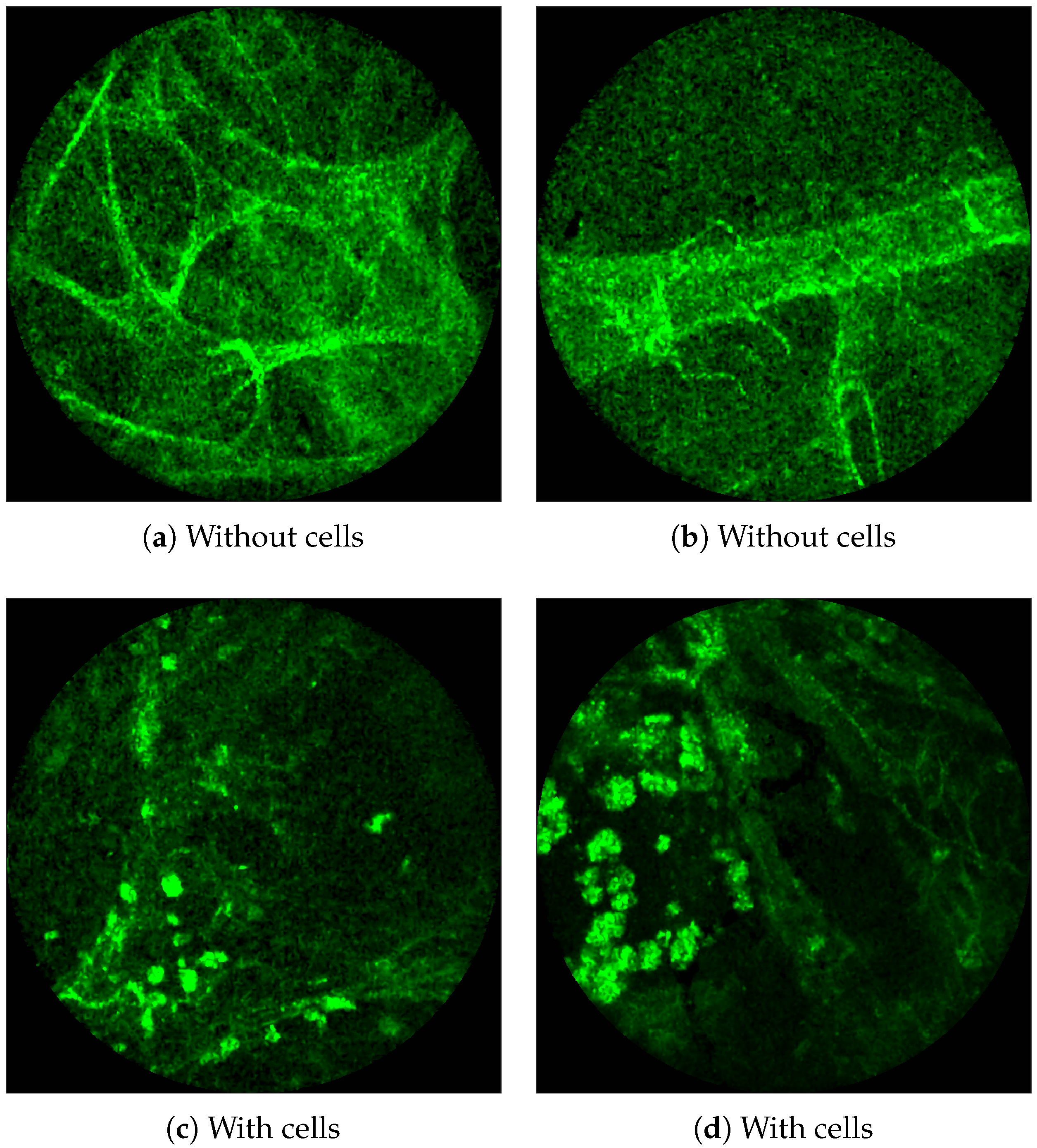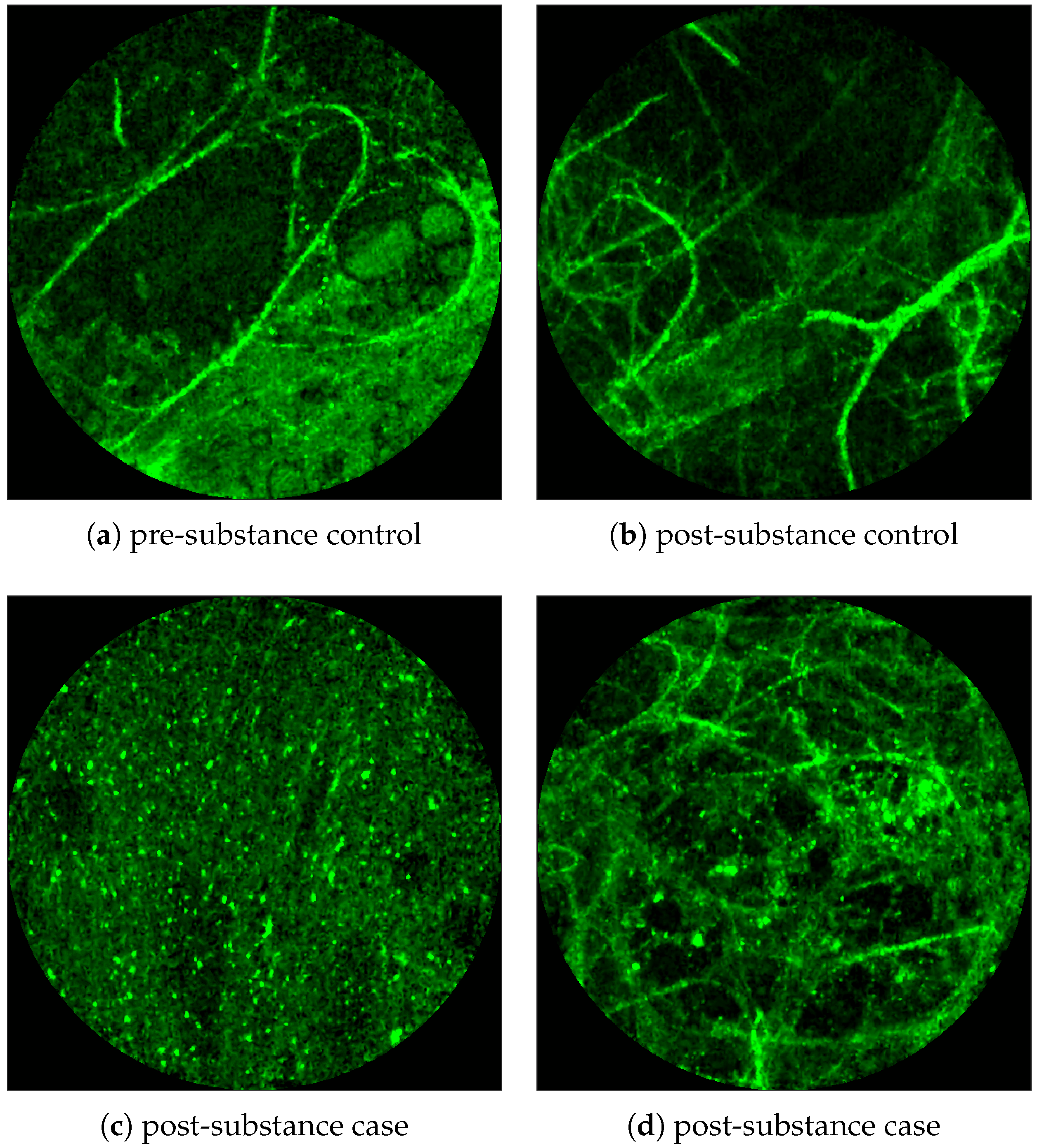Figure 1 and Figure 2 show examples of FCFM images. Human lungs display a mesh-like structure due to autofluorescence of the connective tissues called elastin. For example, elastin is visible in Figure 1a and Figure 2a,b.

The standard methods of detecting bacteria or cells in the human lungs are histopathology and bronchoalveolar lavage (BAL). Histopathology is an invasive approach where a biopsy is performed to extract a sample of the lung which is then studied for the presence of diseases, whereas in BAL, fluid is instilled in a small area of the lung, and then collected for examination [2,3]. However, these approaches are time consuming and can have variable sensitivity [4]. FCFM allows an alternate minimally-invasive approach to image the distal lung in high resolution and can take advantage of using additional imaging agents to detect bacteria or specific cellular phenotypes, can provide information in near real-time, and the procedures are repeatable, allowing monitoring of disease processes. The distal lung represents the gas-exchanging acinar units where pathologies such as pneumonia and acute respiratory distress syndrome occur. Optical imaging of the distal lung has only been made possible by passing small FCFM fibres down the endobronchial tree [5].

FCFM imaging and the autofluorescence of the human lung have been used to explore ‘abnormalities’ without the need of invasive approaches. For example, Seth et al., attempt to predict the malignancy of solitary pulmonary nodules from FCFM images [1]. Yserbyt et al., use FCFM to show that the presence of cells, which autofluoresce as well, can be a sign of acute cellular rejection (ACR) [6] (Yserbyt et al., estimate the cellular load in FCFM images manually [6]). Figure 1 shows examples of FCFM images without (top) and with (bottom) cells. The top two images show the elastin and a blood vessel respectively. The elastin structure is also present in the bottom two images, but some additional granular structure is visible in these images that appear due to the presence of cells. In general, cells appear as round objects.

FCFM imaging has recently gained prominence in investigating the presence of bacteria using targeted smartprobe [7]. Smartprobes are specialized molecular agents introduced in the imaging area to make the bacteria fluoresce. Since the diameter of a bacterium (1–2 microns) is usually smaller than the width of the fibre core as well as the gap between two consecutive fiber cores (about 3 microns), it appears as a high intensity dot of the same size as the fibre core in the image frame and, tends to ‘blink’ on and off in consecutive image frames due to movement of the apparatus. Figure 2 shows examples of FCFM image frames without (top) and with (bottom) bacteria. Human lungs display autofluorescence with or without the presence of smartprobe whereas bacteria appear as dots in the image frame when exposed to smartprobe (Figure 2c). However, one can observe bacteria-like dots in the absence of the smartprobe as well due to noise (Figure 2a). Additionally, if bacteria are present, they are usually easy to detect when the elastin structure is not prominent (Figure 2c), but it becomes more difficult to discriminate them from the background in the presence of elastin structure (Figure 2d).

We address the task of estimating bacterial and cellular load in a FCFM image frame. We consider a formal approach to the bacteria and cell detection problem by explicitly annotating bacteria and cells in image frames, and use this knowledge in a supervised learning set-up to learn a classifier that assigns a probability value to each pixel of the image of a bacterium or cell being present. Estimating bacterial and cellular load can generally be framed as a learning-to-count [8] problem where we need to count the bacteria or the cells. However, although the learning-to-count framework usually bypasses the problem of detection before counting, we suggest detecting the object to allow the clinicians to see where the bacteria or cells are appearing, ideally while performing the bronchoscopy. That said, our method bears resemblance with the established learning-to-count approaches with the major difference being that we learn a classifier to predict a probability value at each pixel whereas the other approaches learn a regressor to predict the ‘count density’ (intensity value) at each pixel (see Section 2.9).

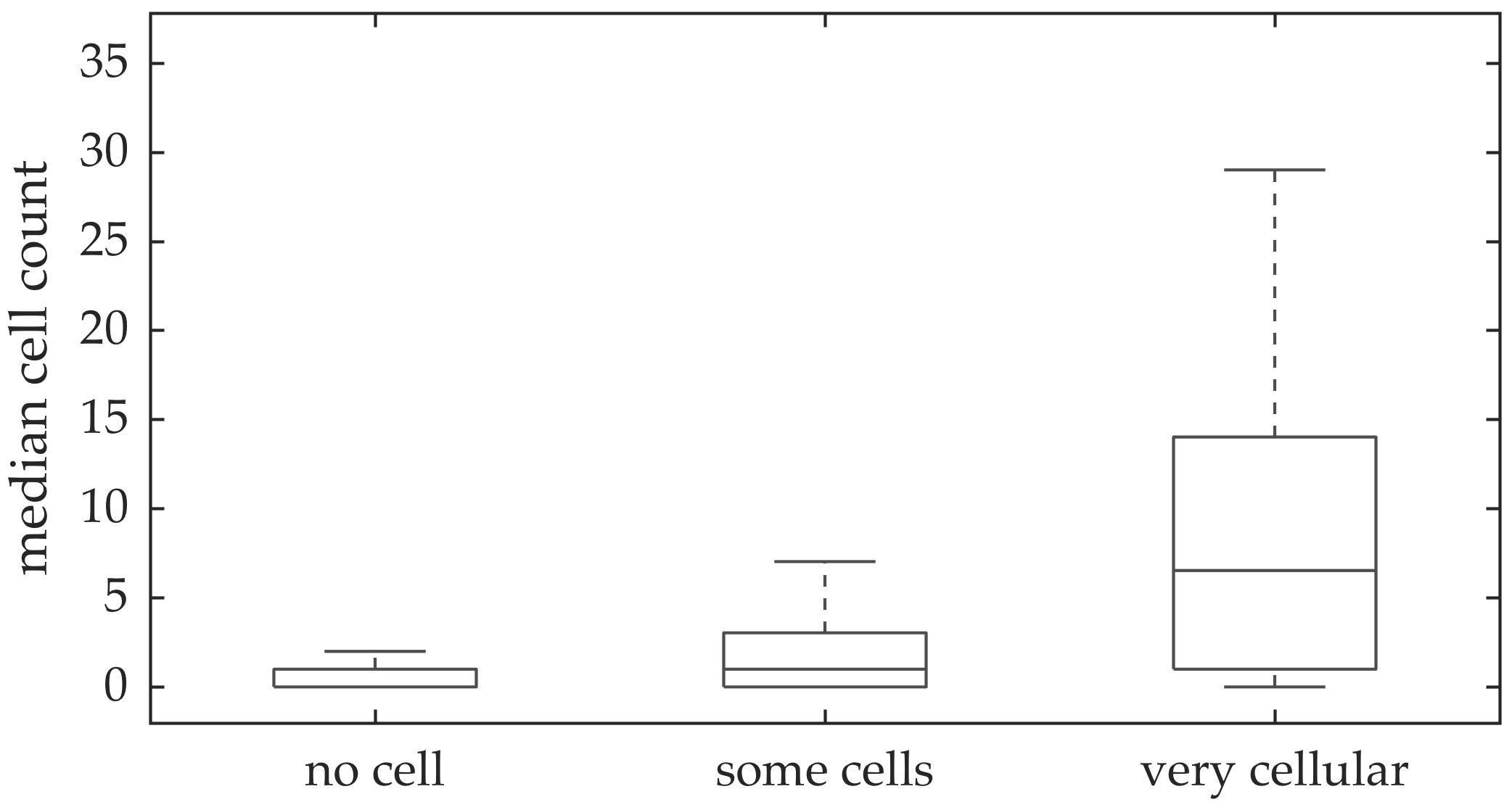
Our ultimate goal is to build a real time system to assist clinicians in estimating bacterial and cellular load while performing bronchoscopy. We suggest using a multi-resolution spatio-temporal template matching scheme using radial basis functions. Spatio-temporal analysis allows better capturing of the ‘blinking’ effect of a bacterium, whereas multi-resolution analysis allows better discrimination between bacterial dots or cellular structure and elastin background. We use normalized intensity values around each pixel as features, which enables fast implementation of our method using 2D-convolutions. We apply this method in estimating bacterial load in FCFM videos with and without bacteria (case and control), before and after applying the smartprobe, and show that we successfully infer low bacterial load in the control or the pre-substance videos and high bacterial load in the post-substance videos from the cases. We also apply this method in estimating cellular load in FCFM image frames with and without cells, and show that the estimated cellular load agrees with the visual assessment of a clinician (We do not have access to the ground truth in the sense that we do not know whether a video should or should not have cells present by experimental design).

2. Materials and Methods

2.1. Collection

2.1.1. Bacteria Dataset

In vivo imaging was performed using Cellvizio System in 6 patients (3 cases with gram-negative bacteria where a bacterial signal was detected and 3 cases with gram-positive bacteria (controls) where signal was not detected) where measurements were taken before and after administration of a gram-specific bacterial specific smartprobe (pre- and post-substance measurements respectively). We refer to these 12 videos as the first cohort. A further 5 patients were assessed with suspected pneumonia, of which two demonstrated a bacterial specific signal post-substance. We refer to these 10 videos as the second cohort. Each measurement is a FCFM video (12 frames per second, about 500 frames per video) that were manually cleaned to ensure alveolar imaging by removing motion blur, air imaging, bronchi etc, and the remaining clean frames were used for this study (For an online implementation, the proposed algorithm can be used in conjunction with methods to remove uninformative frames automatically, e.g., as proposed in [9]).

2.1.2. Cell Dataset

In vivo imaging was performed in 102 patients who have had bronchoscopy. The video frames were curated, i.e., they were relatively free of noise, motion blurs, and artifacts. Although cells can be seen in some of the FCFM frames, we do not have any ground truth if certain videos should have more cells than the others. A clinician assessed the cellular load visually for the videos, and gave each a score between 0 and 2 with 0 implying no cells detected, 1 implying some cells detected, and 2 implying that the video is very cellular.

2.2. Annotation

The learning-to-count problem can be addressed in a variety of different annotation scenarios among which two widely used ones are the dot-annotation and the count-annotation [10]. While dot-annotation provides the location of where an object appear in the image, count-annotation only provides the number of objects in an image without explicitly revealing the locations. We use dot-annotations since they are more informative given the small size of the objects we are trying to count.

2.2.1. Bacteria Dataset

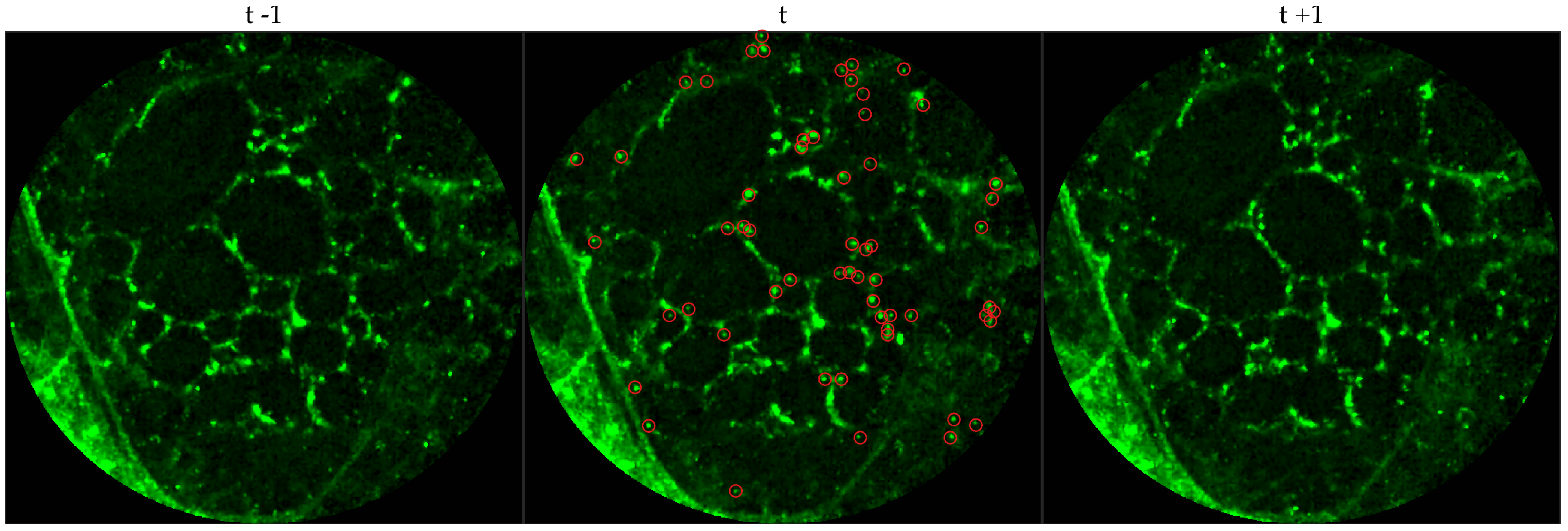
We chose 144 image frames from 12 videos in the first cohort such that 72 of them come from videos without bacteria (8 frames from 9 videos that are either in the control group or in the pre-substance group), and 72 of them come from videos with bacteria (24 frames from 3 videos that are in the post-substance case group). Along with the 144 image frames, the previous and next frames corresponding to those frames were extracted as well, and the clinician was allowed to toggle between the previous and next frame to annotate a bacterium in the current frame. Thus, a bacterium was identified in a spatio-temporal context. 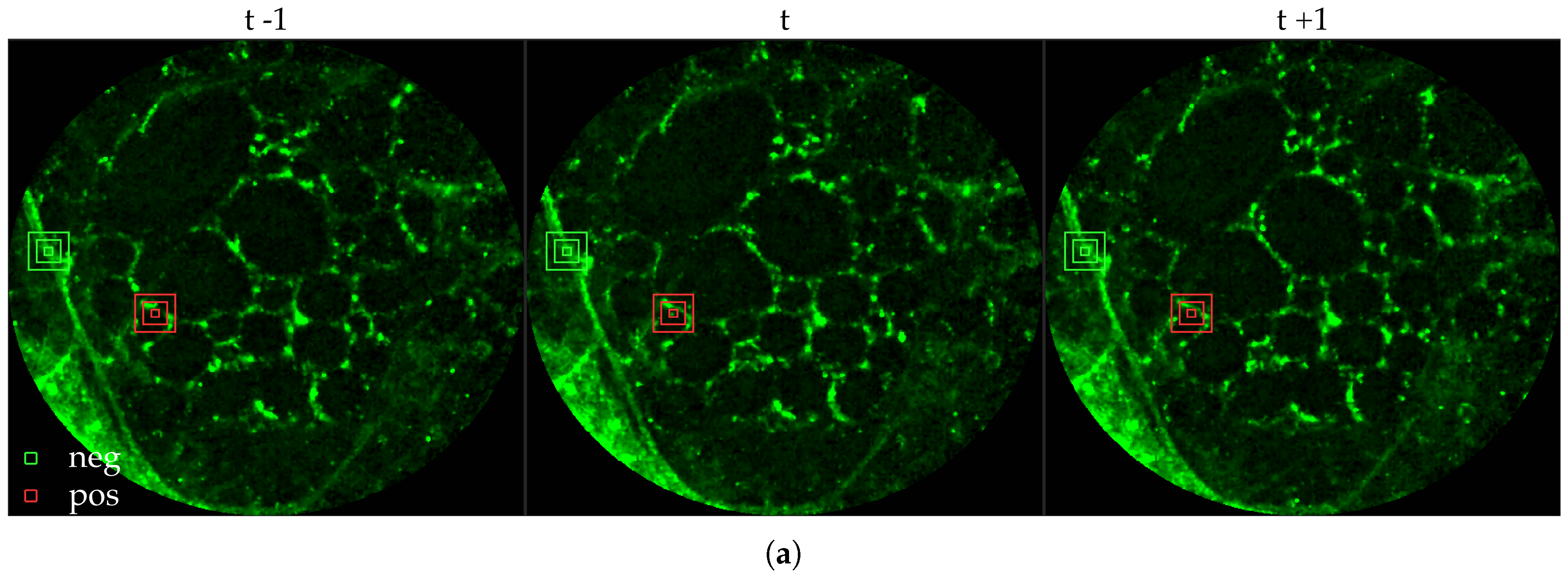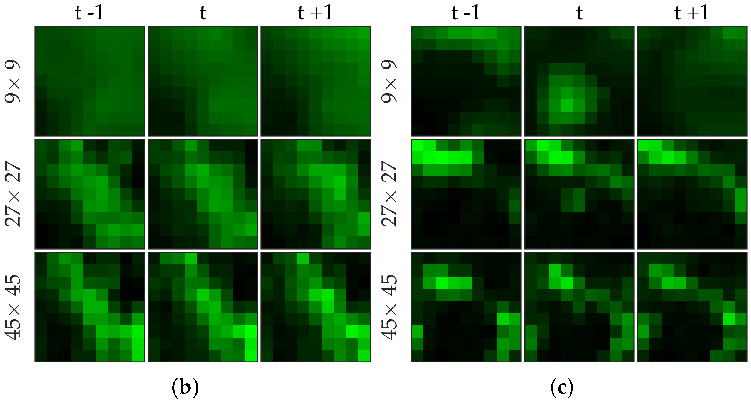Figure 3 shows an example of an annotated frame along with respective previous and next frames to demonstrate the blinking effect.

2.2.2. Cell Dataset

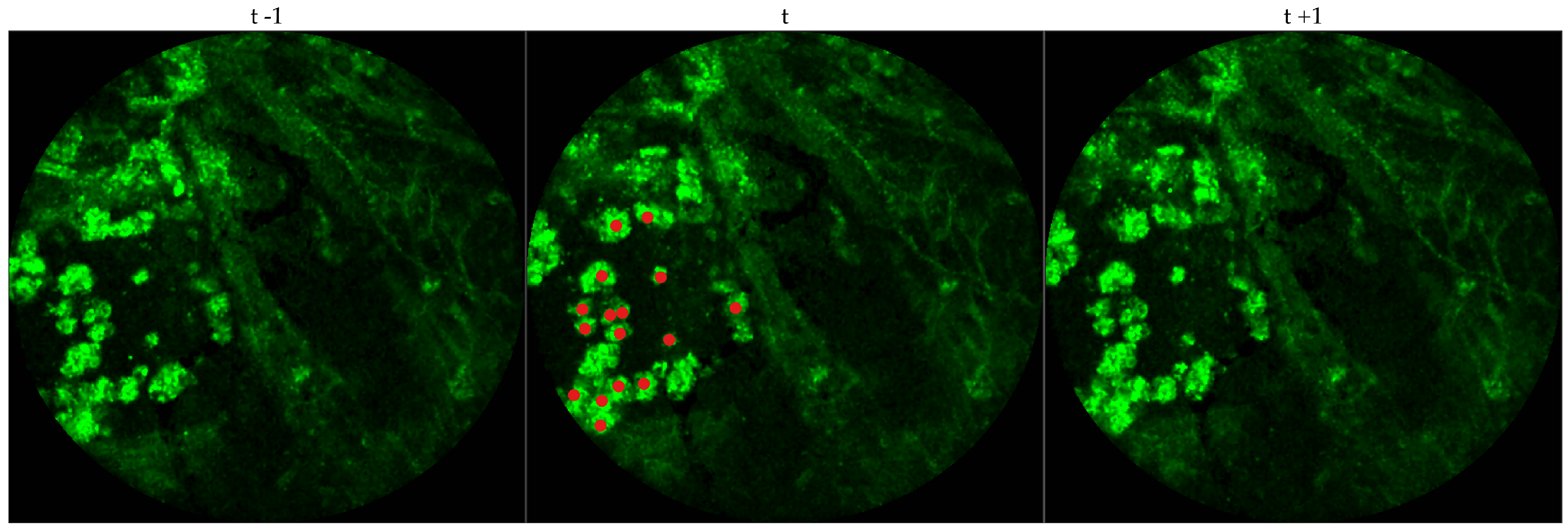
We chose 333 images frames from 216 videos (There can be multiple videos for each patient). We have access to the cellularity score of each patient which indicates the cellularity detected. We extracted one frame for each video with zero cellularity score, and four frames for each video with non-zero cellularity score. Similar to bacteria dataset, the previous and next frames corresponding to the 333 frames were extracted as well, and a cell was identified in a spatio-temporal context. 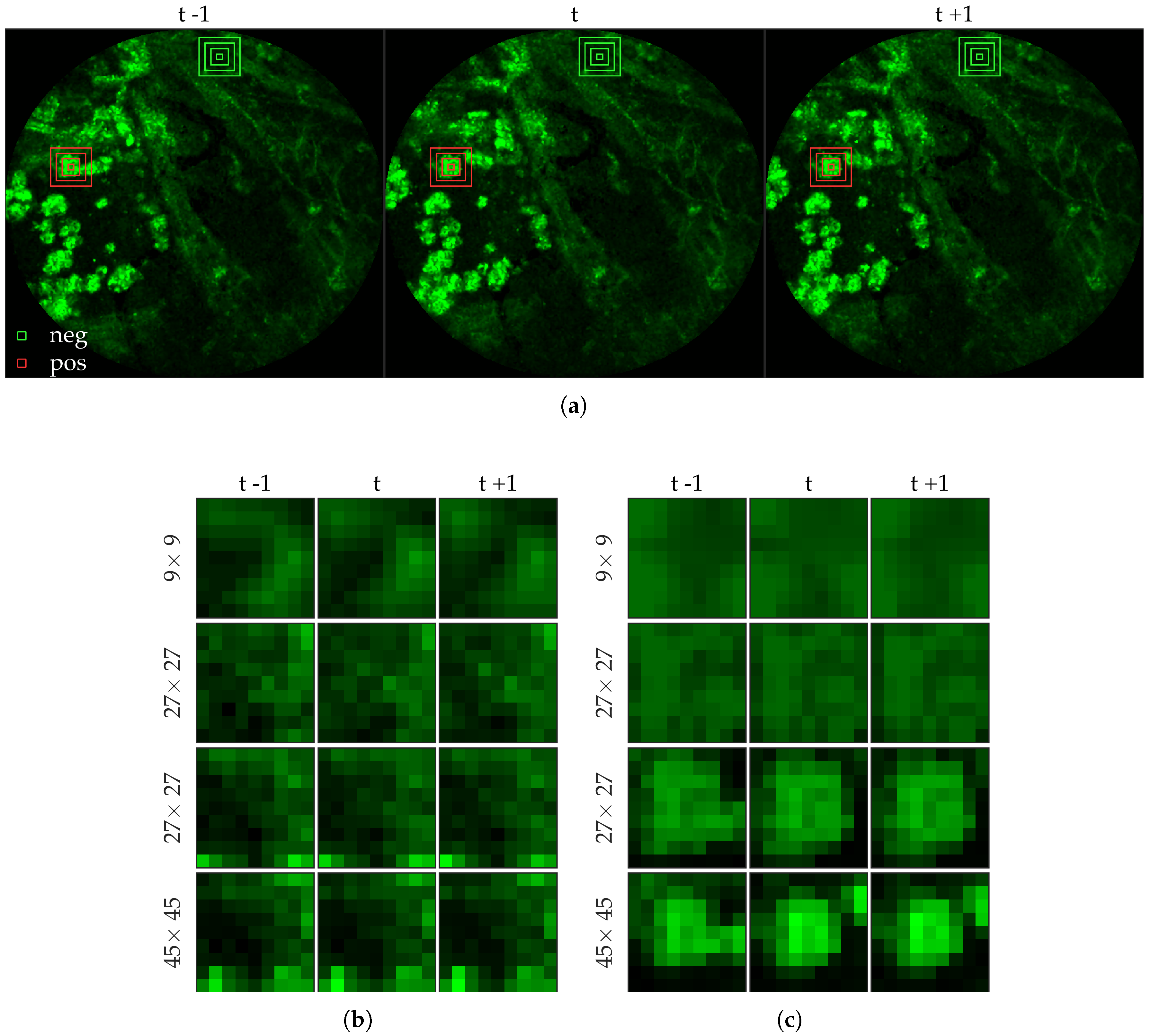Figure 4 shows an example of an annotated frame along with respective previous and next frames.

We observe that although we might encounter false positives, i.e., bacteria are annotated in either control group or pre-substance group, the clinician successfully annotates more bacteria in the frames where bacteria should exist, i.e., post-substance case group. For training purposes we only considered positive annotations from the post-substance case group. A similar observation cannot be made for the cell dataset due to the lack of ground truth, however, false positives and false negatives can be expected given that not all videos are of high quality.

2.3. Preprocessing

To reduce the effect of noise and spurious intensity values we adjust the lowest and highest values of each image frame individually as follows: for each image frame, first, we set any intensity values below $1\%$ quantile to 0, and next, we set any intensity values above $99\%$ quantile to the respective $99\%$ quantile values (This also increases the dynamic range, and thus helps the clinicians in annotating).

To allow supervised learning, we associate a feature vector ${\mathbf{x}}_p$ and label $y_p$ to each pixel in the image and group the pixels in positive ($y_p=1$) and negative samples ($y_p=0$). We use the intensity values over a patch around a pixel as feature vector. However, we observe that image patches can vary significantly in contrast and therefore, we normalize them by the total intensity of the patch as follows: given an image patch ${\{{\tilde{x}}_{ij}^p\}}_{i,j=1}^w$ of size $w\times w$ around pixel p, we normalize the patch as $x_{ij}^p={\tilde{x}}_{ij}^p/{\sum }_{ij}({\tilde{x}}_{ij}^p+ϵ)$ where $ϵ=1$ is added to suppress noisy image patch, i.e., ${\tilde{x}}_{ij}^p\approx 0$. Thus, our basic feature vector is ${\mathbf{x}}_p=(x_{11}^p,\dots ,x_{ij}^p,\dots ,x_{ww}^p)$. $y_p=1$ if p has been annotated by the clinician and 0 otherwise.

For positive labels ($y_p=1$), we pool all image patches around the pixels annotated by the clinician. For negative labels ($y_p=0$), we extract equispaced image patches over a grid ($15\times 15$ pixels apart). If any of the ‘negative’ image patches have a bacterium, they were assigned to the positive samples. Along with the original image patches, we performed data augmentation by rotating each image patch by 90, 180 and 270 degrees and adding them to the pool of samples. This results in about 18,000 positive samples and 540,000 negative samples for the bacteria dataset, and 2500 positive samples and 1,600,000 negative samples for the cell dataset. Notice that our classes are severely imbalanced: we use undersampling of the negative class to maintain a class balance while training a classifier.

For temporal analysis, we extract patches around the same pixel from the previous and the next image frame, normalize them individually and concatenate them to the feature vector from the current frame. For multi-resolution analysis, we extract larger image patches and ‘downsample’ them to the size of the smallest patch. This is done to allow equal importance over each resolution. These patches are normalized individually and concatenated to the feature vector. We ‘downsample’ the larger image patch, usually $t\in \{3,5,7,\dots \}$ times larger than the smallest image patch, by averaging over a $t\times t$ window, e.g., $3\times 3$ or $5\times 5$ window around the pixel (in the patch) being downsampled. Figure 5 shows examples of positive and negative image patches for the bacteria dataset. We observe that (i) dot annotations can be noisy in the sense that the pixel with a bacterium might not be centered, and (ii) larger patch captures the context whereas smaller patch captures the object. 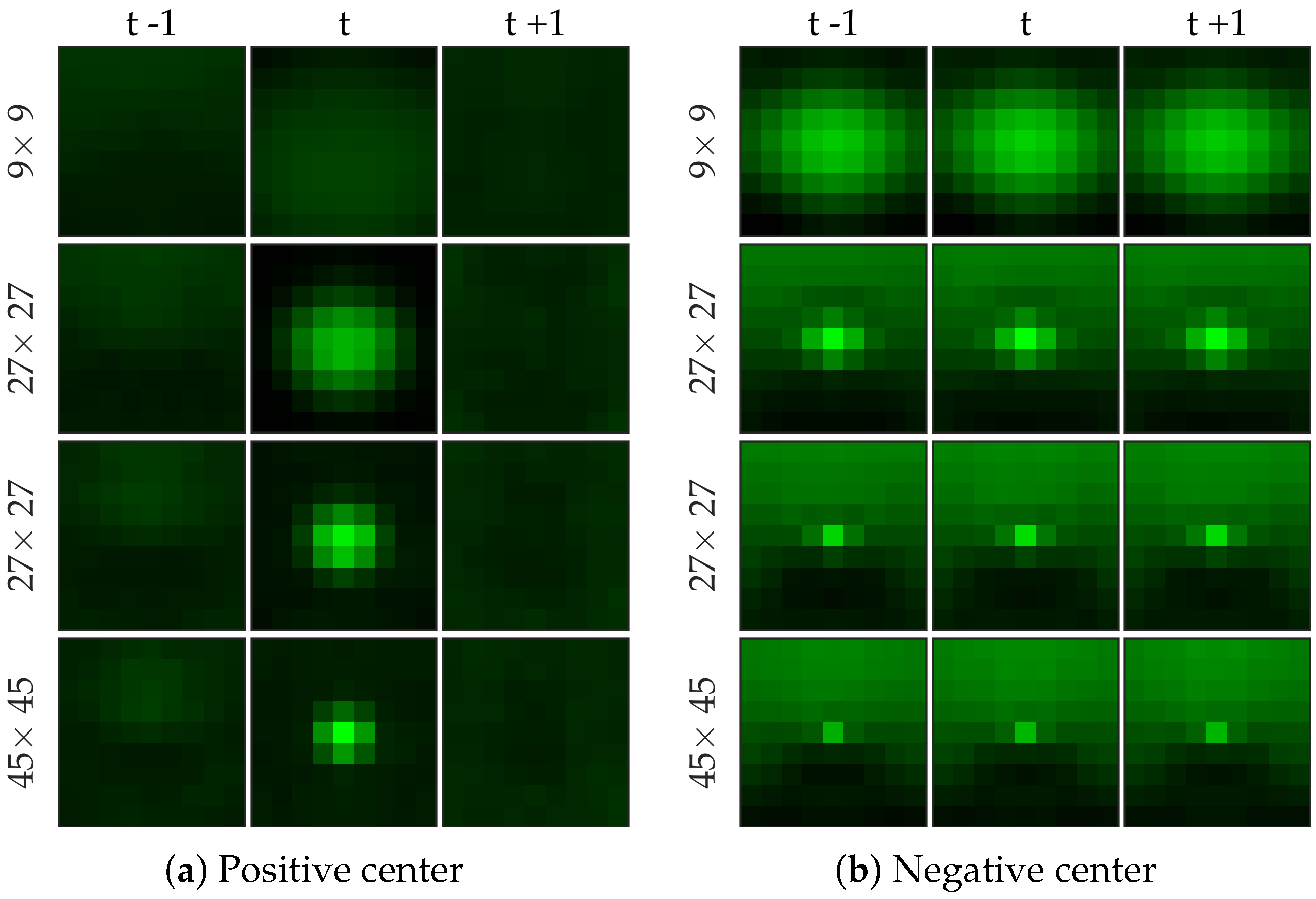Figure 6 shows examples of positive and negative image patches for the cell dataset. We observe that since cells are much larger than bacteria, they are visible only in a larger image patch. However the smaller patches are nonetheless important since they are able to differentiate between a ‘smaller’ cell-like structure, and an actual cell.

2.4. Supervised Learning

Our approach is to assign a probability at each pixel of a bacterium being present. Therefore, we essentially solve a classification problem from ${\mathbf{x}}_p$ to $y_p$. For simplicity and ease of implementation, we suggest logistic regression as a baseline method. However, we observe that it performs rather poorly. We then suggest radial basis functions network [11] as an alternative, and show that it improves the performance significantly.

2.4.1. Logistic Regression

We solve a $L_2$ regularized logistic regression (LR) to learn a linear classifier, i.e.,

$$\begin{array}{c}\hfill \underset{\mathbf{w},b}{min}-\frac{1}{\left|\mathcal{P}\right|}\sum _{p\in \mathcal{P}}\left(y_{p}log\sigma ({\mathbf{w}}^{\top }{\mathbf{x}}_p+b)+(1-y_p)log(1-\sigma ({\mathbf{w}}^{\top }{\mathbf{x}}_p+b))\right)+\frac{\lambda }{2\left|\mathcal{P}\right|}{\left|\right|\mathbf{w}\left|\right|}^2\end{array}$$

where $\sigma$ is the sigmoid function and $\mathcal{P}$ is the set of all pixels in either positive or negative samples, and $\lambda$ is the regularization parameter. We set $\lambda =0.01$. Since we have class imbalance, we resample the negative samples to maintain class balance.

We test the performance of the baseline method with three different choices of features on the bacteria dataset (since the cell dataset has fewer positive samples) (i) with $9\times 9$ image patches extracted from the current frame, i.e., ${\mathbf{x}}_p\in {\mathbb{R}}^{81}$, (ii) with $9\times 9$ image patches extracted from the current as well as previous and next frame, i.e., ${\mathbf{x}}_p\in {\mathbb{R}}^{81\times 3}$, and (iii) with $9\times 9$ and $45\times 45$ image patches extracted from the previous, current and future frames, i.e., ${\mathbf{x}}_p\in {\mathbb{R}}^{81\times 6}$. We expect (ii) to perform better than (i) since it captures the blinking effect, whereas (iii) to perform better than (ii) since it provides more contextual information around a bacterial dot.

2.4.2. Radial Basis Function Network

We learn a radial basis function network (RBF) as a nonlinear classifier where the input vector ${\mathbf{x}}_p$ is first transformed through a set of nonlinear transformations, or radial basis functions, ${\varphi }_i\left({\mathbf{x}}_p\right)$ before being used as the input to the classifier, i.e., we solve the same problem as in logistic regression but replace the original feature vector ${\mathbf{x}}_p$ with the output of the radial basis functions ${\left\{\varphi ({\mathbf{x}}_p-{\mathbf{c}}_i)\right\}}_{i=1}^{64}$ where ${\mathbf{c}}_i$ are centers of the radial basis functions. In other words, we model the output y as

$$y\sim \mathrm{Bernoulli}\left(\sigma \left(\sum _{i=1}^{64}\varphi (\mathbf{x}-{\mathbf{c}}_i)+b\right)\right)$$

instead of a linear model $y\sim \mathrm{Bernoulli}({\mathbf{w}}^{\top }\mathbf{x}+b)$ where $y\sim \mathrm{Bernoulli}\left(p\right)$ denotes the Bernoulli random variable with probability of success p.

For $\varphi$ we used a Gaussian kernel with bandwidth set to median intersample distance. We chose the centers of the radial basis functions using k-means [12]. Since we have many fewer positive samples than negative, we chose 16 centers from the positive samples and 48 centers from the negative samples. Figure 7 shows examples of centers chosen from positive and negative samples for the bacteria dataset. 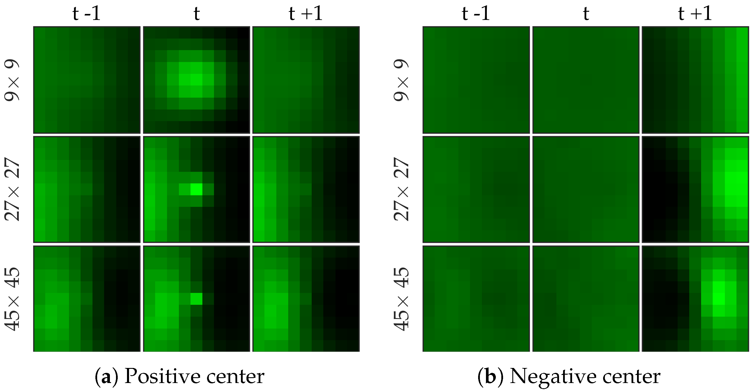Figure 8 shows examples of centers chosen from positive and negative samples for the cell dataset (Figure 8b shows a template learned to be not a cell, and it looks very similar to a cell template but only smaller). After choosing the centers, we perform logistic regression from 64 dimensional feature vector to the class label to learn the weight vector of the network. Notice that for selecting the centers we used the entire (after cross-validation split) negative set rather than undersampled set that we use for learning the weight vector.

We test the performance of the RBF network on the bacteria dataset with two different choices of features, (i) with $9\times 9$ image patches extracted from the current as well as previous and next frame, i.e., ${\mathbf{x}}_p\in {\mathbb{R}}^{81\times 3}$, and (iii) with $9\times 9$, $27\times 27$ and $45\times 45$ image patches extracted from the previous, current and future frames, i.e., ${\mathbf{x}}_p\in {\mathbb{R}}^{81\times 9}$. We expect (ii) to perform better than (i) since it captures more contextual information around a bacterial dot. Additionally, we expect RBF network to perform better than linear logistic regression since it effectively uses 64 ‘templates’ than one (weight vector in the linear classifier). We test the performance of the RBF network on the cell dataset (i) with $9\times 9$, $27\times 27$ and $45\times 45$ image patches extracted from the current frame, i.e., ${\mathbf{x}}_p\in {\mathbb{R}}^{81\times 3}$, (ii) with $9\times 9$, $27\times 27$ and $45\times 45$ image patches extracted from the previous, current and future frames, i.e., ${\mathbf{x}}_p\in {\mathbb{R}}^{81\times 9}$ (iii) with $9\times 9$, $27\times 27$, $45\times 45$ and $63\times 63$ image patches extracted from the current frame, i.e., ${\mathbf{x}}_p\in {\mathbb{R}}^{81\times 4}$, and (iv) with $9\times 9$, $27\times 27$, $45\times 45$ and $63\times 63$ image patches extracted from the previous, current and future frames, i.e., ${\mathbf{x}}_p\in {\mathbb{R}}^{81\times 12}$. We expect (iii)–(iv) to perform better than (i)–(ii) since cells are larger objects which requires a larger image patch to provide contextual information, and (ii)–(iv) to perform similar to (i)–(iii) since cells do not have the blinking effect, and therefore, temporal information might not play a crucial role.

2.5. Postprocessing

The classifier returns a probability value at each pixel. These probability values are then thresholded, and pixels that exceed this threshold value are counted after non-maximum suppression [13] to estimate bacterial load.

2.6. Evaluation Method

2.6.1. Performance Metric

We compare different methods in terms of the precision-recall curve for varying thresholding of the probability map before non-maximum suppression. Given a contingency table of false positives, true positives, and false negatives, precision P and recall R are defined as follows.

$$P=\frac{\mathrm{TP}}{\mathrm{TP}+\mathrm{FP}},R=\frac{\mathrm{TP}}{\mathrm{TP}+\mathrm{FN}}.$$

Given the locations of pixels where an object (bacterium or cell) has been detected and the annotations by the clinician, we draw a disk of radius r around the annotations, and if a detection exists within the disk then it is declared to be a match as in [14].

• If a detection does not match any ground truth. annotation, then it is declared to be a false positive.
• If a ground truth annotation does not match any detection then it is declared to be a false negative.
• If a detection exclusively matches a ground truth annotation and vice versa, then the detection is declared to be a true positive.
• If multiple detections exclusively match a ground truth annotation, then one of them is declared to be a true positive while the rest are declared to be false positives.
• If multiple ground truth annotations exclusively match a detection, then the detection is declared to be a true positive while the rest of the ground truth annotations are declared to be false negatives.
• If multiple detections and multiple ground truth match each other non-exclusively then their assignments are resolved greedily. Notice that the assignment might not be optimal.

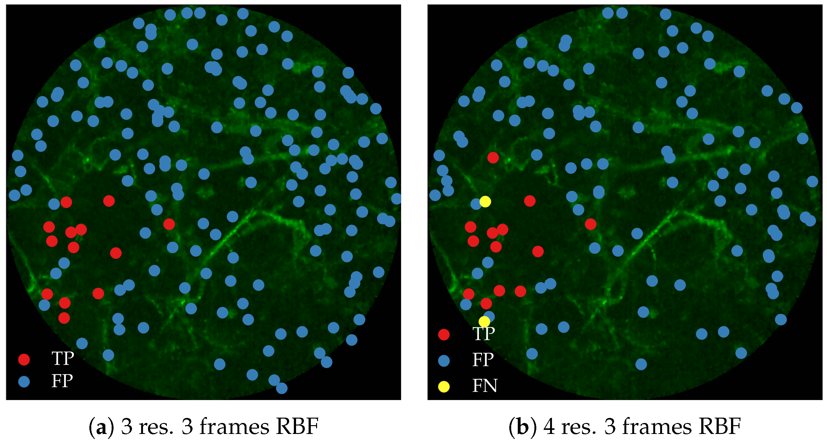
Figure 9 illustrates these different situations. We set $r=4$ pixels.

2.6.2. Precision-Recall Curves

We utilize cross-validation to test the performance of the methods. To elaborate, we divide 144 (333) image frames in 5 groups ${\mathcal{C}}_i,i=1,2,3,4,5$. To learn the probability map for image frames in group ${\mathcal{C}}_i$ we train a classifier with positive and negative samples extracted from the remaining four groups ${\mathcal{C}}_j,j\ne i$. After repeating this process for each group, these probability maps are treated as the output of the classifiers, and the precision-recall curve is estimated by computing the false positive, false negative and true positive values over all image frames.

2.7. Cross-Validation Results for Bacteria Detection

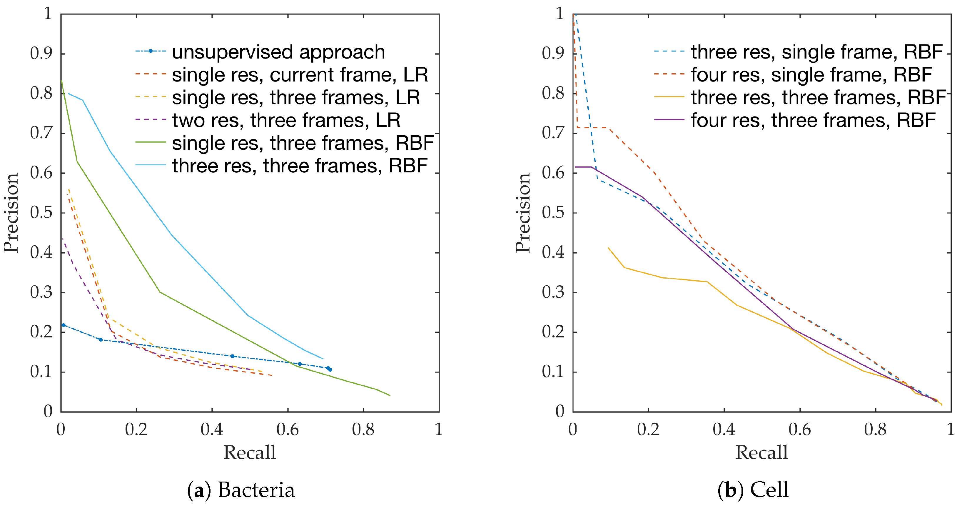
Figure 10a shows the precision-recall curves from all learning methods and feature extraction strategies. We observe the following,

• RBF network performs better than linear logistic regression
• Using temporal information enhances performance. This can be seen from the performance of logistic regression with and without temporal information.
• Using multiple resolution enhances performance. This can be seen from the performance of RBFs with and without multiple resolutions.

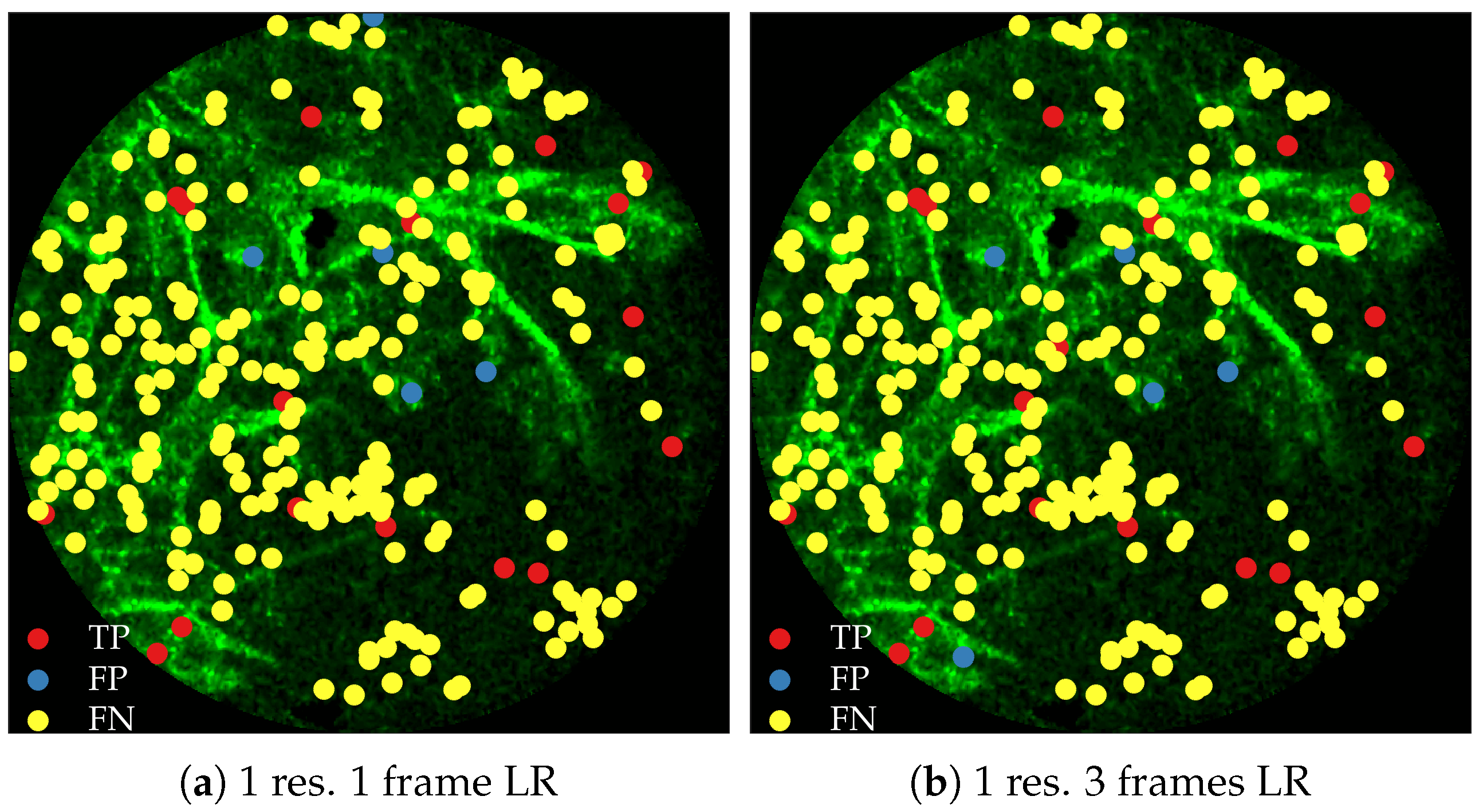
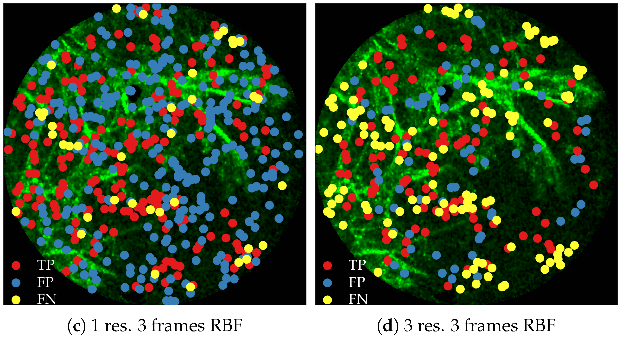
This follows the intuition behind the use of spatio-temporal multi-resolution analysis. Figure 11 compares annotations by the clinician and detections made by the learning algorithms on one of the validation image frame. We observe more true positives for RBF with multi-resolution spatio-temporal analysis.

2.8. Cross-Validation Results for Cell Detection

Figure 10b shows the precision-recall curves for RBF method using different feature extraction strategies. We observe the following,

• Using larger spatial window improves performance. This can be seen for both with and without the use of temporal information.
• Using temporal information degrades performance. This can be seen for both cases of spatial resolutions.

We expect the performance to increase with spatial resolution since higher resolution provides better context. On the contrary, cells do not move as much between consecutive frames as bacteria do, and therefore, temporal information might not be as useful in this context as in bacteria detection. Figure 12 compares annotations by the clinician and detections made by the learning algorithm on one of the validation image frame.

2.9. Related Work

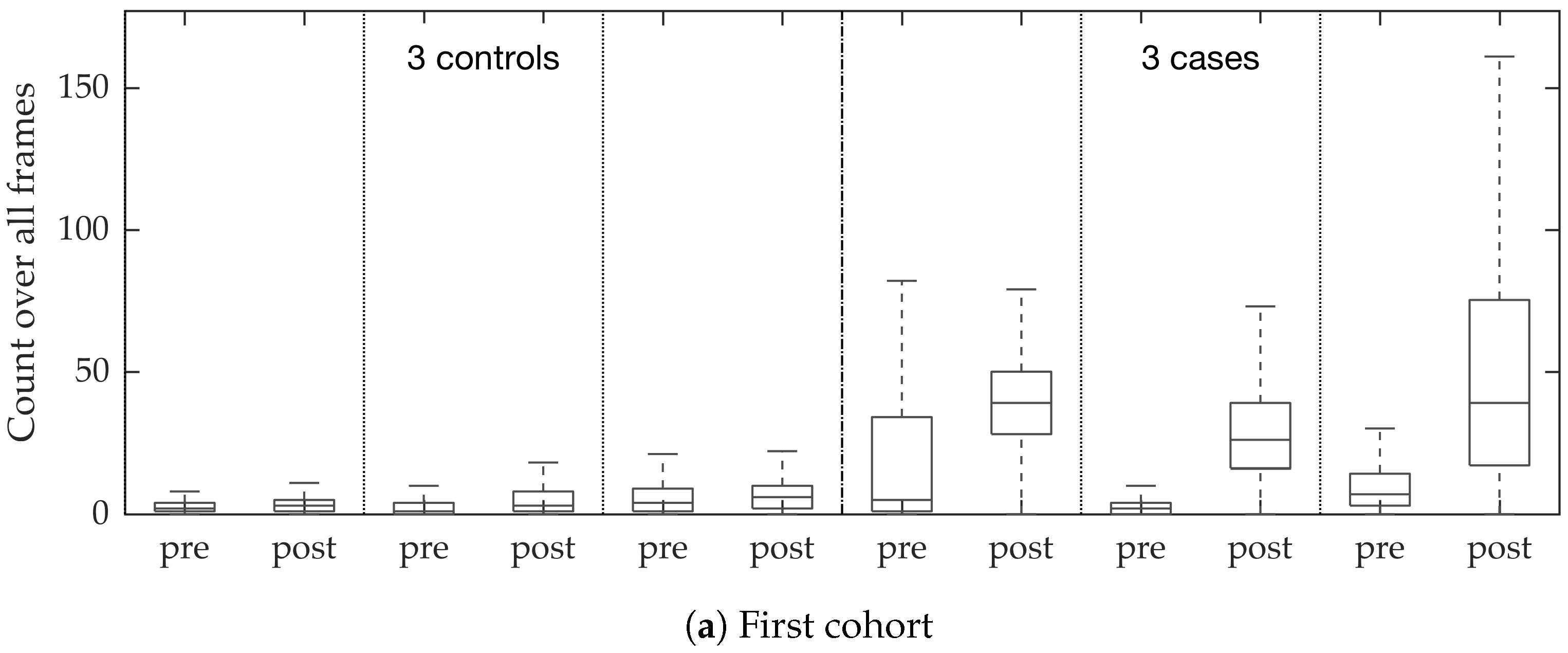
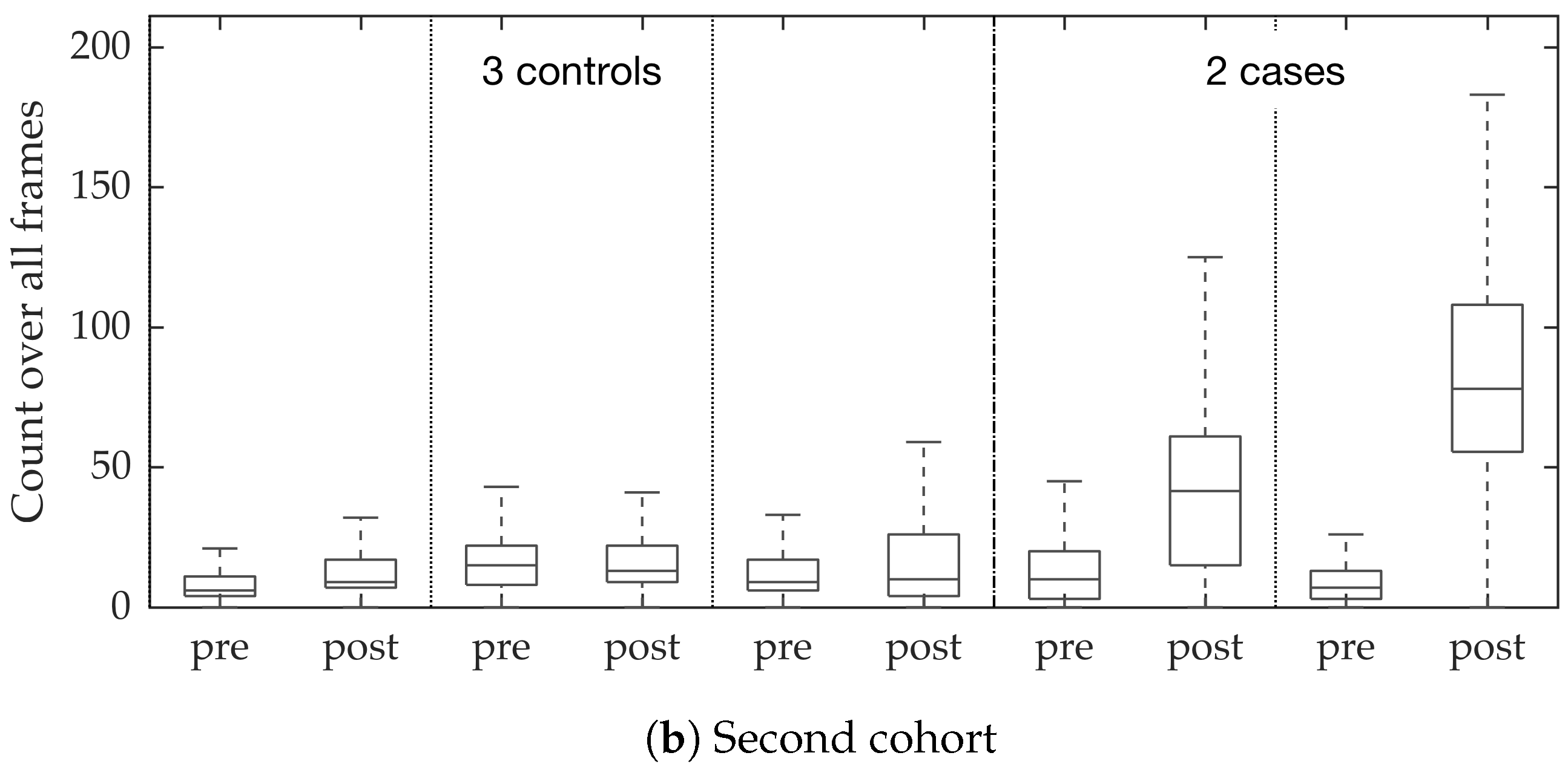
Estimating bacterial load has previously been addressed in our group using an unsupervised learning set-up where difference of Gaussians features were used to enhance the dots in the image. We assessed the precision-recall curve for the unsupervised approach in the context of the acquired ground truth annotations, as presented in Figure 10. We observed that the proposed supervised approach outperforms the unsupervised approach significantly. We also demonstrated the performance of the proposed method using fold change of bacterial load in control and case groups before and after the application of the smartprobe. In the control group, the estimated bacterial load did not change much when exposed to the smartprobe, whereas in the case group the estimated bacterial load showed a significant change. Although the results showed the desired performance in case vs. control group in pre- vs. post-substance measurements, the method tended to overestimate bacterial load in an image frame.

Arteta et al., tackle the problem of object counting as density estimation, known as density counting, where integrating the resulting density gives an estimate of the object count [8]. The authors extract image patch based feature vector (Contrast-normalized intensity values at each pixel in the patch after rotating the patch by the dominant gradient) ${\mathbf{x}}_p$ at each pixel p and construct a dictionary (512 elements) via k-means with $l_2$ distance. Each feature vector is then mapped to a binary vector ${\mathbf{z}}_p$ via one-hot encoding based on its smallest $l_2$ distance to the dictionary elements. The authors suggest learning a regression model from ${\mathbf{z}}_p$ to $y_p$. This, however, may lead to overfitting due to matching the density value at each pixel. Instead the authors suggest matching the densities such that they should match when integrated over an extended region which leads to a smoothed objective function, and is equivalent to a spatial Gaussian smoothing (Arteta et al. [8] suggest using the width of the kernel to be greater than half of the typical object diameter) applied to each feature vector and response vector before applying ridge regression. Essentially, the algorithm constructs a set of templates, and each template is assigned a probability value corresponding to the learned weight vector. Given a test image patch first the closest dictionary element is found, and the related probability value is assigned to the patch. Our approach is similar to [8] in the sense that we work with dot annotations. However, we learn a classifier instead of a regressor, and explicitly detect where each bacterium or cell appears.

Following the work from [8], Arteta et al., address learning-to-count penguins in natural images [15]. The authors have access to around 500 thousands images, and each image has been dot-annotated by a maximum of 20 annotators. The authors use multi-task learning through convolutional neural network to, (1) separate foreground containing penguins from background, (2) estimate count density within foreground region, and (3) estimate variability in annotations in foreground region ([15] Figure 2). We do not use a convolutional neural network due to lack of training images frames.

3. Results

Figure 13 and Figure 14 summarize the main result of the paper for bacteria and cell datasets respectively.

3.1. Case vs. Control Study for Bacterial Load

We analysed 22 FCFM videos from 11 patients (5 cases with bacterial detection and 6 cases without bacterial detection (controls)). For each patient, two measurements were taken, i.e., before and after application of the targeted smartprobe. Since bacteria do not autofluoresce, they can only be detected after applying the smartprobe. Therefore, only the post-substance videos should have a significant non-zero bacterial load. Out of these 22 videos, 12 videos (first cohort) were analysed earlier in our previous study [16] where a classifier was learnt from annotating randomly chosen image frames from the cohort. In the current study, we apply the classifier learnt on the first cohort to the remaining 10 videos (second cohort). Figure 13 shows the estimated bacteria loads in the two cohorts. As expected, we observe that the estimated bacterial load shows significant change from pre- to post-substance in the case group as opposed to the control group (Notice that for both bacterial and cellular load estimation, even though a video has bacteria or cells present, it might have some image frames without bacteria and cells, thus resulting in a low bacterial or cellular count for those image frames in the video).

3.2. Clinician Consensus for Cellular Load

We analysed 206 FCFM videos from 102 patients who have undergone bronchoscopy and FCFM. Some of these videos have cells present and some do not. However, since it is not a controlled study, we do not have the ground truth of which video should have cells and which should not. An independent clinician (different from the annotator who annotated image frames for training) annotated the videos according to their level of cellularity, i.e., amount of cells present. The videos either contain no cell, some cells or they are very cellular. Figure 14 shows the median cell count of videos for each of these cellularity levels. We observe that the median cell counts follow an increasing trend over these three categories, i.e., the cellular load estimated by the proposed method agrees with the visual assessment of the clinician.

4. Discussion

We address the task of estimating bacterial load in FCFM images using targeted smartprobe, and estimating cellular load in FCFM images using autofluorescence. We create a database of annotated image frames where a clinician has dot-annotated bacteria or cells, and use these databases to train a radial basis function network for estimating bacterial or cellular load. We show that spatio-temporal features along with multi-resolution analysis can better predict the bacterial load since they capture the ‘blinking’ effect of the bacteria, and provide better contextual information about the bacterial dot and cellular structure. An attractive aspect of the suggested method is that it can be implemented efficiently using convolutions since it estimates the inner product between image patches to compute the outcome of the radial basis functions. We apply the suggested method in estimating bacterial load at each image frame of FCFM videos from control and case group. We observe significant fold change in the case videos before and after introducing smartprobe, which is not observed in the control group. We also apply the same approach in detecting cellular structure, and show that the estimated cellular load agrees with the assessment of a clinician.

While annotating ground truth, it is highly likely that the annotator makes mistakes: (s)he can either falsely annotate a bacterium or cell when it is noise, or simply miss annotating a bacterium or a cell due to their overwhelming numbers in each frame. These types of error are common in any annotation process, but it might have a more severe impact on learning since our objects are ‘dots’ or cells with similar structure: while mis-annotation in other datasets such as penguin or crowd is mostly due to occlusion or objects being far away from the camera (for both cases the features of the object pixels are different from positively annotated objects), for bacteria or cell datasets this is not true. Therefore, wrongly annotated bacteria or cell can assign different labels to same feature vector.

Bacteria can appear on the elastin structure, but we also observe that elastin structure is often misinterpreted as bacterial dots or cells by the classifier, even with the use of more contextual information. One way our method could be extended is by explicitly annotating objects which are misclassified as bacteria or cell but actually part of the elastin structure. This definitely requires extra effort from the annotator, but should improve the performance of the classifier. A potential problem with this approach is that it needs to be revised when more diverse elastin structure becomes available, e.g., patients with granular structure (which arises from smoking). We would need case and control data for this situation in order to cover this scenario. We plan to explore these extensions and limitations as more clinical data becomes available, with the goal of building a robust clinical system. Finally, this study utilises state-of-the-art clinically approved imaging systems, and should future imaging methods improve and change the way that bacteria manifest themselves in the FCFM video, then the system could be retrained to address that.