Pattern Reconstructability in Fully Parallel Thinning

Department of Electrical Engineering, Yuan Ze University, Chungli, Taoyuan 320, Taiwan
*
Author to whom correspondence should be addressed.
J. Imaging 2017, 3(3), 29; https://doi.org/10.3390/jimaging3030029
Submission received: 16 June 2017
/
Revised: 13 July 2017
/
Accepted: 15 July 2017
/
Published: 19 July 2017
(This article belongs to the Special Issue Computer Vision and Pattern Recognition)
Abstract
:It is a challenging topic to perform pattern reconstruction from a unit-width skeleton, which is obtained by a parallel thinning algorithm. The bias skeleton yielded by a fully-parallel thinning algorithm, which usually results from the so-called hidden deletable points, will result in the difficulty of pattern reconstruction. In order to make a fully-parallel thinning algorithm pattern reconstructable, a newly-defined reconstructable skeletal pixel (RSP) including a thinning flag, iteration count, as well as reconstructable structure is proposed and applied for thinning iteration to obtain a skeleton table representing the resultant thin line. Based on the iteration count and reconstructable structure associated with each skeletal pixel in the skeleton table, the pattern can be reconstructed by means of the dilating and uniting operations. Embedding a conventional fully-parallel thinning algorithm into the proposed approach, the pattern may be over-reconstructed due to the influence of a biased skeleton. A simple process of removing hidden deletable points (RHDP) in the thinning iteration is thus presented to reduce the effect of the biased skeleton. Three well-known fully-parallel thinning algorithms are used for experiments. The performances investigated by the measurement of reconstructability (MR), the number of iterations (NI), as well as the measurement of skeleton deviation (MSD) confirm the feasibility of the proposed pattern reconstruction approach with the assistance of the RHDP process.
1. Introduction
The purpose of thinning is to remove a large number of unwanted points for extracting the isotropic thinned skeleton, which shall retain the pattern’s geometrical shape features for computers to efficiently perform image-related tasks, such as character recognition [1,2], fingerprint identification [3], posture recognition [4], retinal image analysis [5], and so on. Over the past half-century, many thinning algorithms have been proposed and can be roughly divided into two main categories: rule-based thinnings (iterative schemes) [6,7,8,9,10,11,12,13,14,15,16,17,18,19,20,21,22,23,24,25,26] and distance-based skeletonizations (non-iterative schemes) [27,28,29,30,31,32,33,34,35,36].
Rule-based thinning applies the thinning templates iteratively to remove the contour points until the unit-width skeleton is obtained. In accordance with the operating manner, rule-based thinning algorithms can be further divided into sequential [6] and parallel [7,8,9,10,11,12,13,14,15,16,17,18,19,20,21,22,23,24,25,26] thinning. For the sequential thinning, the thinning operation of a contour point depends on its neighboring points’ thinning results. The contour points can be removed as long as they are not interior, end and isolated points, in which the removal shall maintain pattern connectivity (for example, eight-connectivity for pattern pixels should be maintained if a (8, 4) binary picture is considered.). On the other hand, parallel thinning can operate the points simultaneously, and one thinning iteration may contain more than one sub-cycle (may also be named as a sub-iteration [7] or pass [12]) or subfield [13,26]. Sub-cycles used in an iteration are often adopted for developing a sub-cycle-based parallel thinning, where the operator/reduction may be changed with a period of 2, 4 or 8. For example, two-sub-cycle thinning removes symmetrically and iteratively the contour points from two opposite erosive directions until the thinned result converges to be of unit-width. If a thinning algorithm uses one sub-cycle, it is a fully-parallel algorithm. For a one-sub-cycle thinning as defined by Chen and Hsu [9], a contour point whose erosive direction is the same as its neighboring points can always be removed regardless whether the current iteration count is even or odd. Otherwise, if its erosive direction differs from one of its neighboring points, its removal is dependent on whether the current iteration count is odd or even like the checking in the two-sub-cycle scheme for the preservation of line connectivity. For a subfield-based (or subfield-sequential) algorithm, the binary picture is partitioned into more than two (say k) subfields, which are alternatively activated. During a given iteration step, k successive parallel reductions associated with these subfields are performed, and some pattern pixels in the active subfield can be designated for removal [13,26]. In order to generate the suitable deletion rules for parallel topological algorithms, some sufficient conditions for topology-preserving parallel reductions were proposed by Németh et al. [22]. Based on the sufficient conditions, fifty-four 2D parallel thinning and shrinking algorithms were constructed; and a four-sub-iteration scheme with intermediate deletion directions and the iteration-level endpoint checking in subfield-based algorithms were also introduced [22].
A comprehensive survey on thinning methodologies has been reported by Lam and Suen [11]. From the viewpoint of order dependence, the resultant thin line depends on the order of pixels examined in sequential thinning algorithms, whereas that depends on the order of the sub-iterations in parallel thinning algorithms. In order to avoid any kind of order dependence, Ranwez and Soille introduced the concept of order independent homotopic thinning and thus presented an order independent homotopic marking algorithm for thinning [17]. Palágyi further presented a class of equivalent deletion rules and related methods to bridge the order-independent sequential, fully-parallel and subfield-based algorithms [26]. Based on the framework of critical kernels [37], Bertrand and Couprie introduced the notion of crucial pixel to study the framework of digital topology, in which the link between critical kernels, minimal non-simple sets and P-simple points is clarified for thinning algorithm design [21].
For distance-based skeletonization [27,29], the local point with the maximum distance is defined as the skeletal point where distance transformation is performed by finding the shortest distance from the point to its nearest background point. It is the well-known medial axis transformation (MAT) thereafter. A good survey on skeletonization theories, methodologies and their applications can be found in the articles of Saha et al. [35,36]. In accordance with the original MAT definition [27], three important properties in skeletonization are addressed as follows after the investigation of the theory of skeleton and its representation for continuous objects [28,29].
- The connectivity of the derived skeleton is preserved as long as the original object is connected.
- The original object can be exactly reconstructed from its skeleton.
- The geometry of the skeleton is invariant under picture rotation.
However, while considering the digitized plane, the distance-based skeletons are usually discrete, disconnected, as well as not of unit-width. This means that the three properties mentioned above are not easily maintained due to the effect of discrete metrics as investigated by the literature [31,38,39]. In order to render the advantage of the low boundary noise effect from the MAT and overcome the disconnected issue, a MAT-based thinning has been proposed by Chen and Chao [40]; who also argue a new challenge of “is it possible that the original line pattern can be completely restored with the thinned result?” Up to now, this issue is not easy for a conventional rule-based thinning algorithm since no reconstructable information is preserved, but the line connectivity during the thinning process. Therefore, the goal of this paper is to propose a pattern-reconstructable strategy embedded in a rule-based thinning so that a good thinning result can be maintained, as well as the original pattern can be reconstructed from the built thin line information (in MAT-based skeletonization, the pattern can be reconstructed from its MAT by a re-expansion process as mentioned by Peleg and Rosenfeld [30], whereas the pattern reconstruction from the built thin line containing the iterative and reconstructable information is considered in this article).
Since Jang and Chin proposed a reconstructable parallel thinning [12] in 1993, there have been very few reconstructable methods regarding rule-based parallel thinning presented and discussed. Jang and Chin’s method is based on a hybrid approach of a fully-parallel thinning algorithm and morphological skeleton transformation (MST). It first identifies a set of disjoint feature pixels containing the required information of reconstruction by means of morphological operations. Then, based on fully-parallel thinning, an iterative boundary removal procedure is adopted for producing a unit-width skeleton. Finally a labeling process is used to encode the resultant skeleton with three information (namely reduced feature pixel, feature pixel and the unit-width pixel obtained by thinning) for pattern reconstruction. Even though the resultant skeleton is connected, unit-width and reconstructable, this method is somewhat complicated for application. The reason is that “skeletons generated by the algorithm vary with different MST structuring templates chosen by the user for the extraction of feature pixels” as discussed by Jang and Chin [12]. Due to the extra feature pixels involved in the traditional skeletal pixels, noisy branches are very easily yielded. Such a phenomenon may easily be observed in a high-resolution pattern. For example, given a binary pattern shown in Figure 1a and performed by the MST-based algorithm, Figure 1c shows the completely reconstructed pattern from the thinned result shown in Figure 1b, where a number of noisy branches are yielded apparently.
In order to avoid the unwanted branches as suffered by Jang and Chin’s method [12], in this study, we present a pattern-reconstructable strategy and hidden-deletable-point removal method embedded in a fully-parallel thinning, where the former can extract the reconstructable information during the fully-parallel thinning process, and the latter can help with reducing the effect of the bias skeleton, thus further improving the reconstruction. Note here that a deletable point, but not be removed in a thinning iteration, is defined as hidden deletable point (HDP), which is usually accumulated in the portion of the L-corner and T-junction, thus yielding the phenomenon of the bias skeleton in a fully-parallel thinning [10,14]. The fundamental principles of designing the presented method are briefly introduced as follows. Basically, in the thinning process, for every iteration, it is of great importance for checking the line connectivity. Let 1-pixel and 0-pixel denote the pattern and background pixel, respectively, in this paper. In order to examine that a 1-pixel P is a deletable point () or has been a skeletal point () in the thinning iteration, a checking function based on the local connecting function defined by Chen and Hsu [9] is reformulated in Section 2 and used in our approach. To make the pattern reconstruction possible, the trajectory of thinning should be recorded. For a 1-pixel P first becoming a unit-width skeletal point, e.g., at the -th iteration, it is regarded as a landmark on the thinning trajectory, and its eight neighbors at the -th iteration will be recorded as the reconstructable information. A RSP (reconstructable skeletal pixel) matrix will be built for storing the thinning flag (The thinning flag F is a trigger-once flag. Initially, it is set to zero. Once a 1-pixel P becomes a skeletal pixel, is set to one eventually during the thinning process.) (F), iteration count (I) and reconstructable information (R). The RSP matrix will be updated after a thinning iteration until the thinning result is not changed, as the flowchart depicted in Figure 2a, where the resultant thin line information is further reduced in a so-called skeleton table, which contains all of the skeletal point’s coordinates, iteration count I and reconstructable R information. In order to overcome the effect of bias skeleton, an HDP removal process can also be involved in the presented flowchart. In this way, both the effect of the bias skeleton and the number of thinning iterations can be further reduced. In accordance with the produced skeleton table, its original pattern can be reconstructed by means of uniting all dilation results for all skeletal pixels with their I and R information, as the flowchart given in Figure 2b.
The rest of this paper is organized as follows. In Section 2, followed by the fundamental definitions, the checking function is formulated, and the RSP information is defined. The RSP updating in a fully-parallel thinning, pattern reconstruction based on skeleton table, as well as HDP removal in thinning iteration are also detailed in Section 2. Section 3 shows experimental results and comparisons. The measurement of reconstructability (MR) [12], the number of iterations (NI) and the measurement of skeleton deviation (MSD) [40] are used for analyses and discussions. The conclusions and future works are finally drawn in Section 4.
2. Proposed Method
In order to facilitate a clear presentation for our method, some definitions shown in [9] are adopted here and given first. Let binary images be composed of two-level pixels; one is the background pixel (or 0-pixel), and the other is pattern pixel (or 1-pixel). For a pixel , let be its eight neighbors as depicted in Figure 3. In this designation, let and denote the sets of integers {0, 2, 4, 6} and {1, 3, 5, 7}, respectively; and be the union set . Moreover, let be the sum of the eight neighbors, which is equal to the total number of 1-pixel neighbors. We can re-index from 0 to for these 1-pixel neighbors in clockwise order and derive a set of integers . Thus, a mapping function is defined to be . Based on these definitions, according to the systematic design of thinning algorithms [9], for the n-th 1-pixel neighbor, its connecting set is defined by:
Based on the , for any two consecutive elements in , take the connecting set of the former element and the location of the latter; the connecting operator ⊗ is expressed by:
Thus, a local connecting () for pixel P is defined by:
In the thinning iteration, the most important thing is that the removal of a 1-pixel P cannot destroy the line connectivity, which can be examined by a checking function . In this study, based on the original definition [9], our checking function is reformulated as below:
where tells that the 1-pixel P is possibly removed (or removable) at the (j)-th iteration. Otherwise, it cannot be removed and has become a skeletal point at this iteration. In the following, the result of the checking function is also named the C-value for convenient presentation.
In order to let the digital pattern be reconstructable from the thinning result, the trajectory of thinning is recorded in our approach. For a 1-pixel first becoming a skeletal point at the -th iteration, for example, it is considered as a landmark on the thinning trajectory as mentioned in Section 1. The reconstructable information at the -th iteration for this landmark should be included, that is for a landmark, its eight neighbors at the -th iteration will be recorded as the reconstructable information. Therefore, in this study, a 16-bit data format shown in Figure 4 is newly defined to represent an RSP-pixel, which consists of the thinning flag (F, bit f), iteration count (I, bits -) and reconstructable information (R, bits -). Each bit indicates the binary value, 0 or 1. The RSP-pixel will be updated in each thinning iteration until the final unit-width thin line is obtained. Here, represents that the 1-pixel has become a skeletal point. I and R can be expressed respectively as follows for converting the value from binary into decimal.
For convenience of presenting our approach, the RSP matrix can also be represented by three matrices (F, I and R).
2.1. RSP Updating in a Rule-Based Thinning
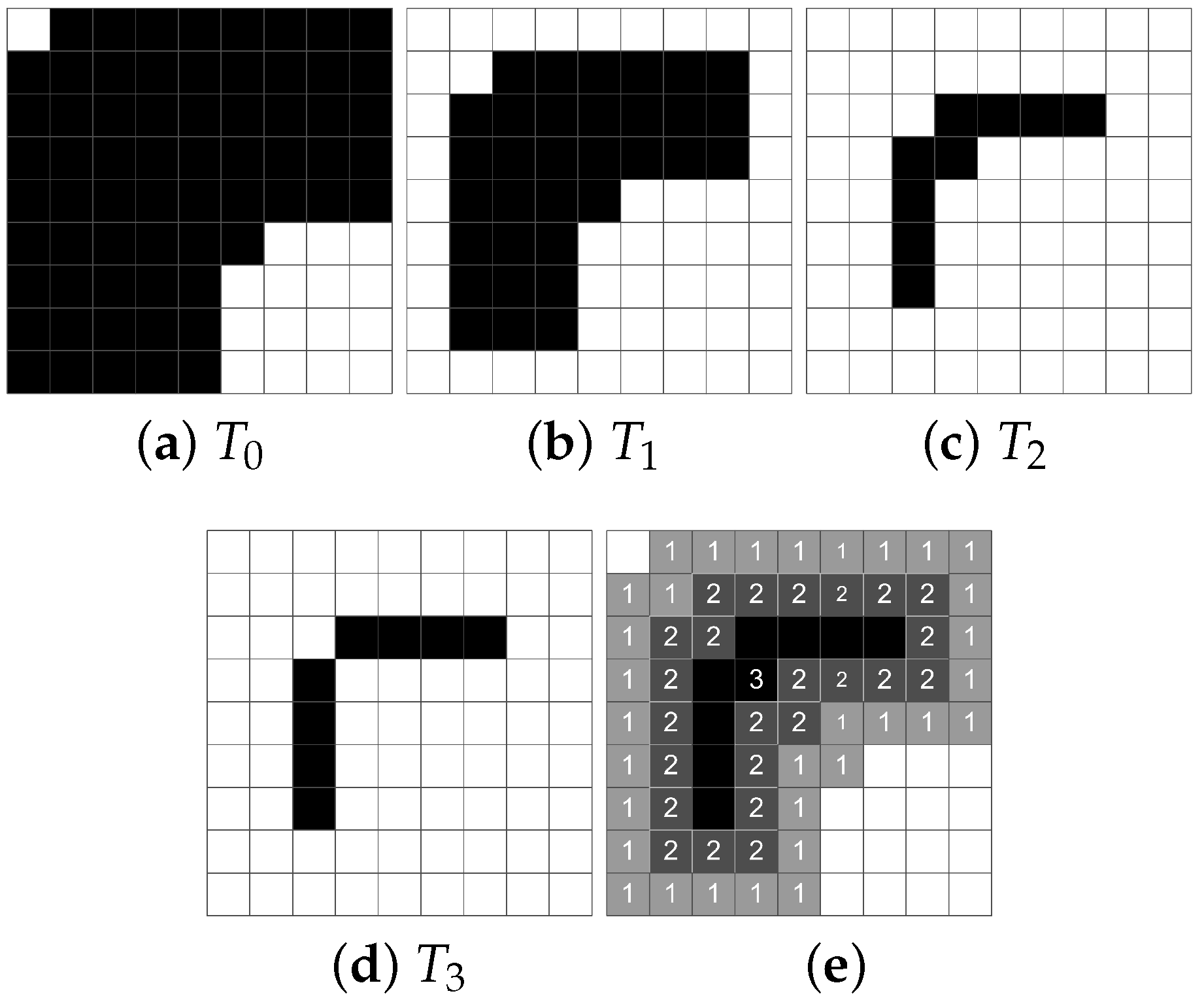
In general, a rule-based thinning applies the thinning templates iteratively to remove the contour points until the unit-width thin line is obtained. For illustrating how to update the RSP matrix in a fully-parallel thinning, a series of iteratively thinning results is given in Figure 5, which are yielded by Chen and Hsu’s method [9] combining with the process of removing HDPs (which will be presented in Section 2.3). Note here that the pixels removed in a thinning iteration are numbered in Figure 5e, which will be helpful for the later presentation.
The mechanism of updating the RSP information for 1-pixel P is presented as follows. Let the RSP matrix be initially set to be null. Let and be the intermediate thinning results at the ()-th and (j)-th iteration, respectively. For a 1-pixel , with the same order as given in Figure 3, let be the P’s eight neighbors and be the reconstructable information for updating. Note here that the pixel could have been a final skeletal point if according to the definition of Equation (4). For a neighbor , the corresponding if it is of 1-pixel and (this means that the 1-pixel neighbor could be possibly removed at the next iteration). Otherwise, means that the neighbor is 0-pixel or has already been a skeletal point satisfying . This can thus be expressed by:
For 1-pixel P, if and , its reconstructable information () is updated as , the iteration information () updated as , as well as is set to 1 (this means that the 1-pixel P has become a skeletal point). Otherwise, remains 0.
Consider the intermediate thinning results and as illustrated in Figure 5c,d, for a 1-pixel denoted in Figure 6b; its eight neighbors are shown in Figure 6a confined by a dotted square. The current iteration count for thinning is . By means of the checking function in Equation (4), we have , , and as the numeric presentation in Figure 6c. Because the thinning flag and , in this case, the reconstructable information is updated as by Equation (7) or further represented as according to Equation (6). The iteration information () is or according to Equation (5). Moreover, since and , the 1-pixel P becomes a skeletal point, and is set to 1. Note here that for a 1-pixel P, once becomes 1, its RSP-pixel updating will not be performed at the following iterations since the necessary reconstructable information of the skeletal pixel, , should be kept at this landmark. Based on the RSP-pixel data format given in Figure 4, in this illustration, is finally updated as (1 000010 00110000), which can also be represented in decimal as (1 2 48) according to Equations (5) and (6).
Based on the operational mechanism presented above, the procedure of updating the RSP matrix in a fully-parallel thinning is summarized as follows.
RSP Updating: Procedure of Updating the RSP Matrix in a Rule-Based Thinning
- Null a RSP matrix.
- Consider the (j)-th iteration in a fully-parallel thinning process. Do Steps 3–5 for each 1-pixel P satisfying and .
- Update according to Equation (7).
- Update .
- Set . This is a landmark that the 1-pixel P first becomes a skeletal pixel.
- Perform Steps 2–5 until the thinning result is not changed. The binary F matrix also represents the final thinning result indeed.
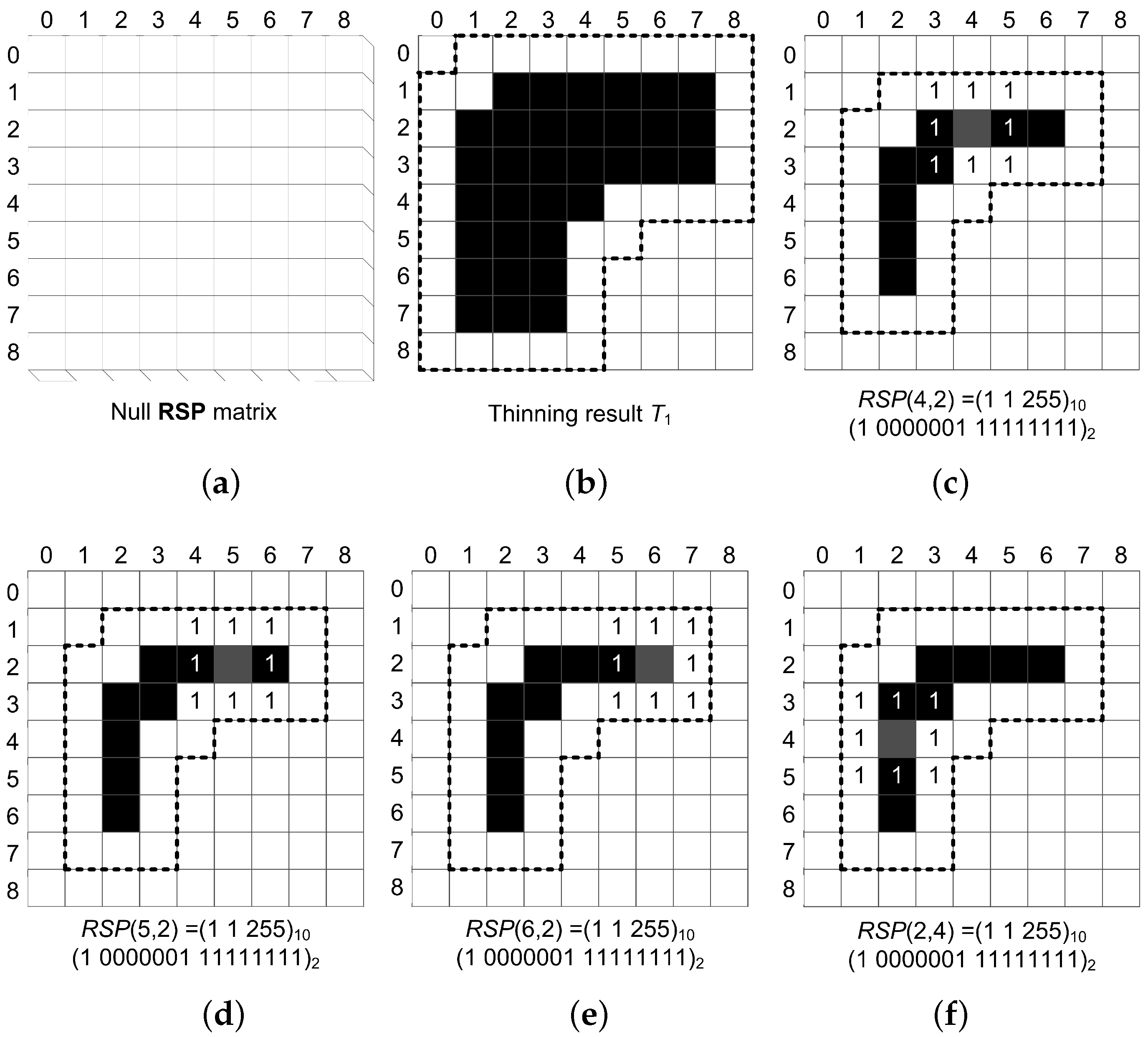
Following the current example, a series of thinning details for each pixel change is given in Figure 7 to illustrate the behavior of RSP updating. Consider a digital pattern as given in Figure 5a; let be the original pattern, and the RSP matrix is set to be null initially, as shown in Figure 7a. After the first thinning iteration, we have the thinning result as shown in Figure 7b, where is confined by a dotted line, and thus, the removed pixel can be easily inspected for reference. There is not any RSP-pixel to be updated in this iteration since the corresponding C-value for every 1-pixel is 1, i.e., all of them are possibly further removed at the next thinning iteration. Figure 7c–h shows the updated RSP information for each 1-pixel P satisfying to in the thinning result (that is, they become skeletal pixels at this thinning iteration), where the reconstructable information is numbered for reference, and the current iteration count is . Note here that for the 1-pixel at (3, 2), (2, 3) and (3, 3), their RSP information is not updated here since their C values are 1. Figure 7i shows the update RSP pixels with gray squares at this thinning iteration. After updating the RSP matrix in , we have just obtained the six skeletal pixels (4, 2), (5, 2), (6, 2), (2, 4), (2, 5), (2, 6), whose C values are 0, and thus, their updates of RSP information stop here.
Consider the next thinning iteration () for the current illustration; let the updated RSP matrix and the thinning result be redisplayed in Figure 8a,b, respectively. Figure 8c,d shows respectively the updated RSP information for the 1-pixel (2, 3) and (3, 2) having zero C value in . Note here that the 1-pixel (3, 3) in the has been removed in . The RSP matrix is finally updated as shown in Figure 8e. The thinning and its RSP updating process stop here for the current illustration. The RSP matrix can be decomposed into F, I and R matrices as shown in Figure 8f,g,h, respectively. This information will be useful for pattern reconstruction as presented in the next subsection.
2.2. Pattern Reconstruction Based on the Skeleton Table
By observing the obtained RSP information, the thinning result can be further represented by a skeleton table, which records only the final skeletal pixels with their coordinates, I and R information as listed in Table 1. The thin line is easily redrawn based on the coordinates in the skeleton table. More importantly, the digital pattern can be further reconstructed based on their I and R information.
According to the RSP-pixel updating as presented in Section 2.1, for each skeletal pixel P, its non-zero neighbors labeled in and iteration count for obtaining its reconstructable structure have been recorded. Therefore, the area of the reconstructed partial pattern for P, denoted as , can be easily performed by just dilating times the non-zero neighbors with a structure element () and expressed by:
where represents that morphological dilations are performed times for each 1-neighbor with the as given below. Then, the union of all dilation results yields the partial reconstructed pattern .
Based on such a pattern reconstruction mechanism, the original pattern can be approximately reconstructed by the following union operation and denoted as , whereas the original pattern is denoted as for the calculation of pattern reconstructability presented in Section 3.
Figure 9 illustrates how to obtain the for all pixels in the skeleton table listed in Table 1. Note here that the reconstructable information 1-neighbor is displayed by a gray square. Except that morphological dilations are performed twice for the cases of Figure 9a,e, it is performed only once for others. The final reconstructed pattern shown in Figure 9i is obtained by the union of all partial patterns ()s and is the same as the original digital pattern given in Figure 5a. The whole procedure of our pattern reconstruction from the skeleton table can be simply summarized as follows.
Pattern Reconstruction: Procedure of Pattern Reconstruction from the Skeleton Table
2.3. Removal of Hidden-Deletable Points in the Thinning Iteration
So far, we have presented how to yield the RSP information during a fully-parallel thinning process and to reconstruct the pattern based on the RSP information. In these illustrations, the used thinning result in each iteration is indeed obtained by means of two processes: the original fully-parallel thinning [9] and the process of removing hidden deletable points (RHDP) newly presented in this section. In the following, we will first examine the effect of our approach without the assistance of the RHDP process, then introduce the so-called hidden deletable point (HDP) and, finally, present our RHDP process.
Reconsider the digital pattern in Figure 5a and perform the fully-parallel thinning [9] on it without the assistance of the RHDP process; the original thinning results in each iteration, denoted by , are shown in Figure 10. Compare them to Figure 5; the results are rather different, and the final thin line is biased obviously. In addition, it takes more thinning iterations (4 versus 3). Figure 10e shows the reconstructed pattern (gray squares) with the presented pattern reconstruction approach, where the result is over-reconstructed. In Chen’s early study [14], this phenomenon results from the so-called HDP effect. Contrary to the complicated vector analysis presented in [14] for detecting the HDPs, in this paper, a simple and feasible way for the removal of HDPs is newly presented as follows.
Recall that denotes the intermediate thinning result at the j-th iteration in Section 2.1. Let be the intermediate thinning result obtained from with only the original algorithm performed. Let be the set of deleted points obtained by performing the set difference between and . Let be the boundary of obtained by first eroding with in Equation (9) and then performing the set difference between and its erosion (). Therefore, we have:
Note here that . Let be the set of points , but ; thus, we have:
It also implies that . Now, consider as an image array with the same size of original image. If the 1-pixel in the -image satisfies , then it is regarded as an HDP, and the corresponding pixel will be removed further. After performing such an HDP removal process as summarized below, the new thinning result can be obtained as used in Section 2.1.
RHDP: Process of Removing HDPs
- Given the intermediate thinning result .
- For each pixel , do Step 4.
- If the pixel P in the -image satisfies , then the corresponding pixel is an HDP and removed from .
- Update for the next thinning iteration.
Figure 11 illustrates how to transform into via the RHDP process. Given as shown in Figure 5a, the next thinning result purely obtained by Chen and Hsu’s method [9] is given in Figure 11a. Thus, we have as shown in Figure 11b according to Equation (11). Based on Equation (12), the boundary of is shown in Figure 11c and denoted by , which can be further displayed as in Figure 11d by labeling the -point and -point. Since the points, (1, 1), (5, 4) and (4, 5), belong to HDPs by means of performing the checking function in Step 4 of RHDP, they can be further removed from , and the new thinning result is thus obtained as shown in Figure 11e, which is the same as in Figure 5b.
3. Results and Discussion
The proposed algorithm is implemented by Microsoft Visual Studio 6.0 C++ and run on a laptop computer with Intel® Core i5 2.6 GHz CPU (Intel, Santa Clara, CA, USA) and 4 GB RAM. Let be the original pattern and be the reconstructed pattern obtained by Equation (10). In order to evaluate the reconstruction ability of the proposed approach, a measurement of reconstructability (MR) [12] is used and expressed as below.
Here, represents the set of pixels , but , and vice versa. The range of MR is between zero and one. The MR increases with the accuracy of reconstructability, where MR = 1 represents that the pattern is reconstructed completely. Since the HDPs removed or not in a thinning iteration will significantly affect the thinning result and number of iterations (NI), the measurement of skeleton deviation (MSD) [40] and NI are also adopted for our performance evaluations. To evaluate the MSD, we can give an original thin line pattern , generate its thick-line pattern by a thickening procedure [14] and perform the by a thinning algorithm to obtain the skeleton result . Then, the MSD can be computed as follows.
where represents the minimum Euclidean distance between q and . In this evaluation, the lower MSD means that the adopted thinning algorithm has a better performance to reduce the bias skeleton.
Reconsider the original digital pattern as given in Figure 1a; by performing the proposed approach on it, the resultant skeletons are shown respectively in Figure 12a without and Figure 12b with the assistance of the RHDP process. The former shows a biased skeleton taking 20 thinning iterations, whereas the latter shows a bias-reduced skeleton taking 14 thinning iterations. In the phase of pattern reconstruction, the reconstructed results are shown in Figure 12c (MR = 0.817) and Figure 12d (MR = 0.994), respectively. Here, we can find that the biased skeleton may result in the over-reconstructed pattern, as shown in Figure 12c. Accordingly, based on these results, not only the feasibility of our pattern reconstruction mechanism is confirmed, but also the developed RHDP process can effectively help to obtain the bias-reduced skeleton and reconstruct the pattern more closely.
3.1. Experiments with a Set of Unit-Width Letters
For investigating additionally the skeleton deviation with MSD, original thin lines should be given initially as ground truths. In this study, we built seven unit-width letters, “A”, “E”, “H”, “L”, “M”, “R” and “T” as shown in Figure 13a. By means of the thickening procedures [14], the thickened results shown respectively in Figure 13b are obtained and will be used for the following investigations of MR, NI, as well as MSD. Since the proposed approach is designed for the fully-parallel thinning algorithms as depicted in the flowcharts of Figure 2, three fully-parallel thinning algorithms, namely CH [9], AW [16] and Rockett [20], are used for comparisons and discussions. Figure 14a,b shows their thinning results without and with the RHDP process, respectively. It is obvious that the biased skeletons of Figure 14b are much less than those of Figure 14a. Note here that in the same test situation, the three algorithms have a similar performance due to such a thinning algorithm based on the similar design rules. This phenomenon can also be reported in the measurements of NI and MSD as listed in Table 2 and Table 3, respectively. Table 2 shows that the average NI with the RHDP process is approximately 27% less than that without the RHDP process. Table 3 shows that the average MSD with the RHDP process is approximately 42% less than that without the RHDP process. Note here that since the Rockett algorithm [20] is the improved version of AW [16], the Rockett algorithm (MSD = 190.7) is a little bit better than AW’s algorithm (MSD = 206.9) by the presented method without using the RHDP process. As a result, this experiment confirms that our RHDP process embedded in a thinning iteration can effectively reduce not only the bias skeleton effect, but also the number of iterations.
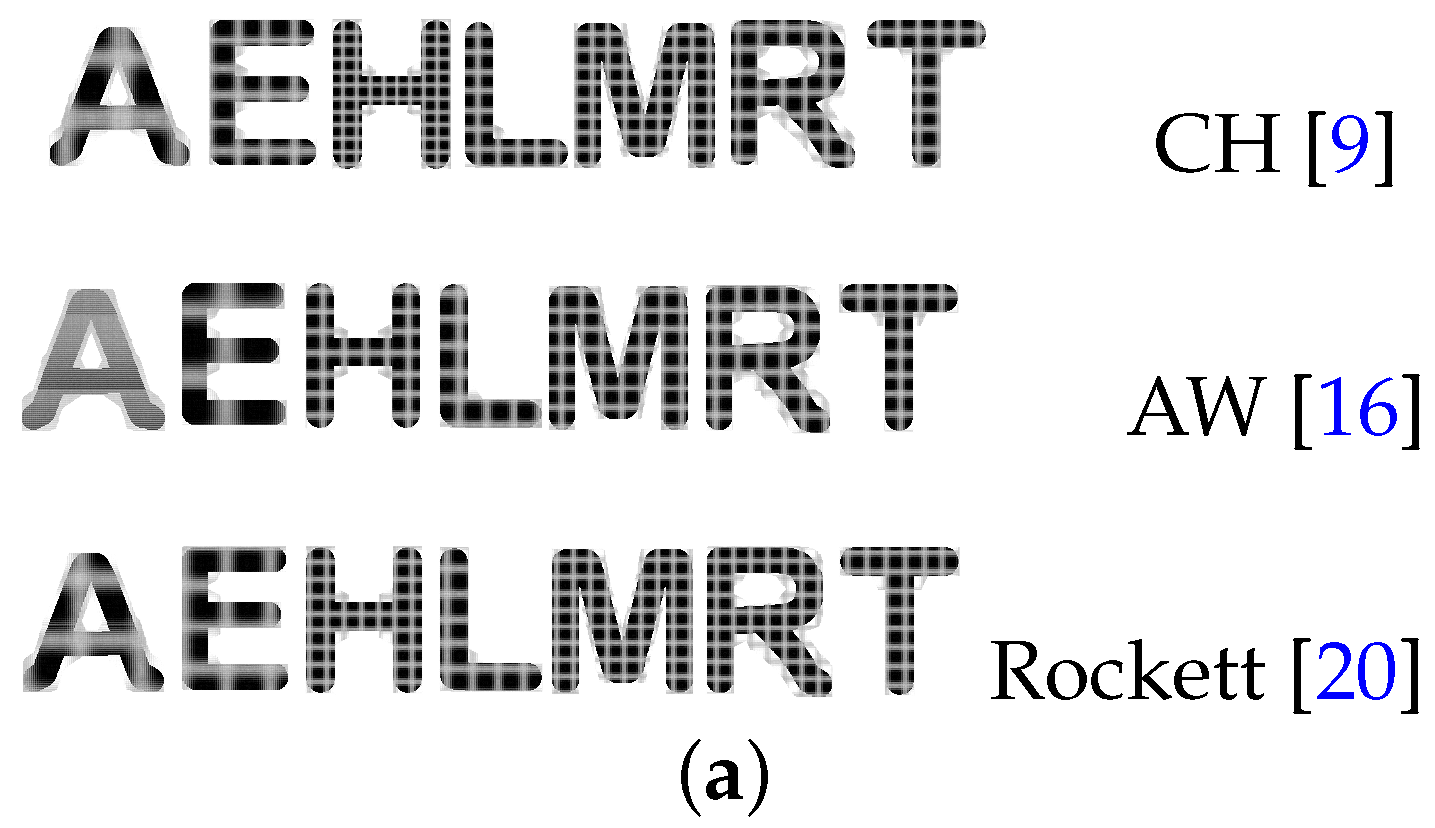
By means of performing the proposed pattern reconstruction approach depicted in Figure 2b on the skeleton tables of the thinning results shown in Figure 14, the corresponding reconstruction results are displayed in Figure 15. It can be seen that the reconstruction results of Figure 15a are over-reconstructed, whereas those of Figure 15b are closer to the originals. Table 4 reports that the average MR with the RHDP process is increased 12.5% compared to that without the RHDP process. This evaluation further confirms that the proposed approach with the assistance of the RHDP process (MR = 0.981) is very feasible for realizing the pattern reconstruction in a fully-parallel thinning.
3.2. Experiments with Some Patterns in the MPEG7 CE-Shape-1 Dataset
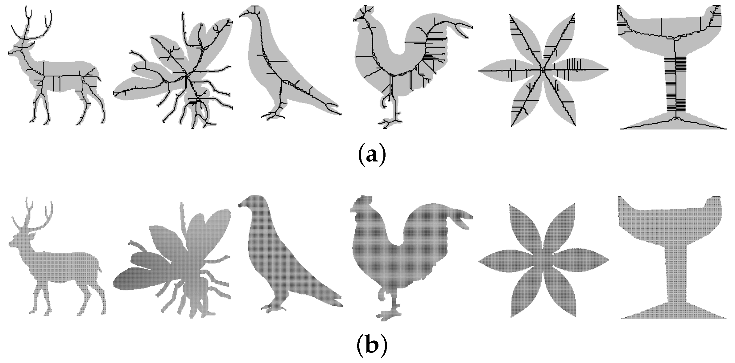
Some patterns (“Deer”, “Fly”, “Bird”, “Chicken”, “Device” and “glass’) from the MPEG7 CE-Shape-1 dataset [41] are used for further experiments and comparisons of the NI and MR measurements. Figure 16a shows the thinning results obtained by applying Jang and Chin’s MST-based reconstructable parallel thinning algorithm [12]. It can be observed that many unwanted branches are yielded in the final skeletons resulting from the fact that the feature points should be retained in the thinning process in order to completely reconstruct the whole pattern as shown in Figure 16b.
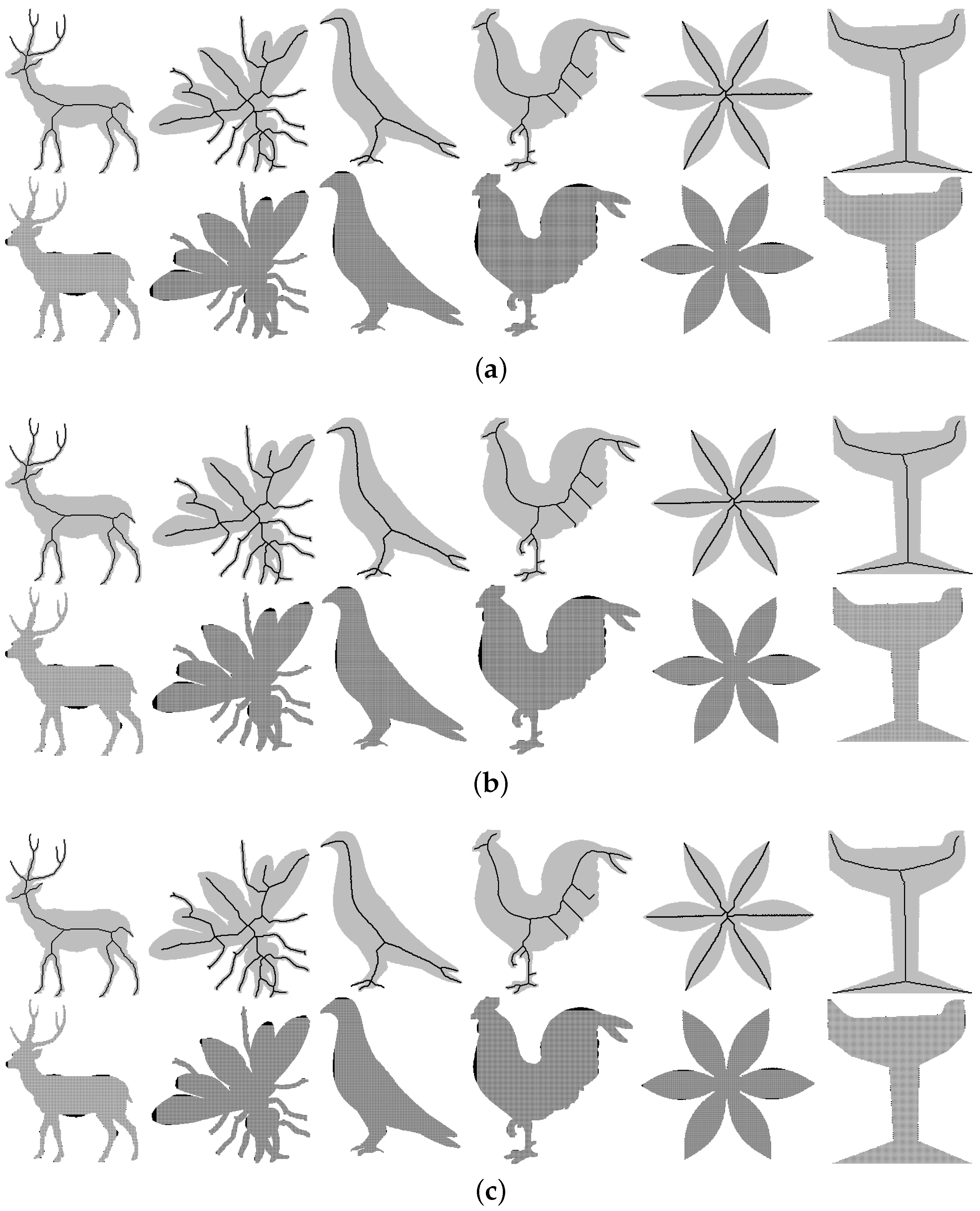
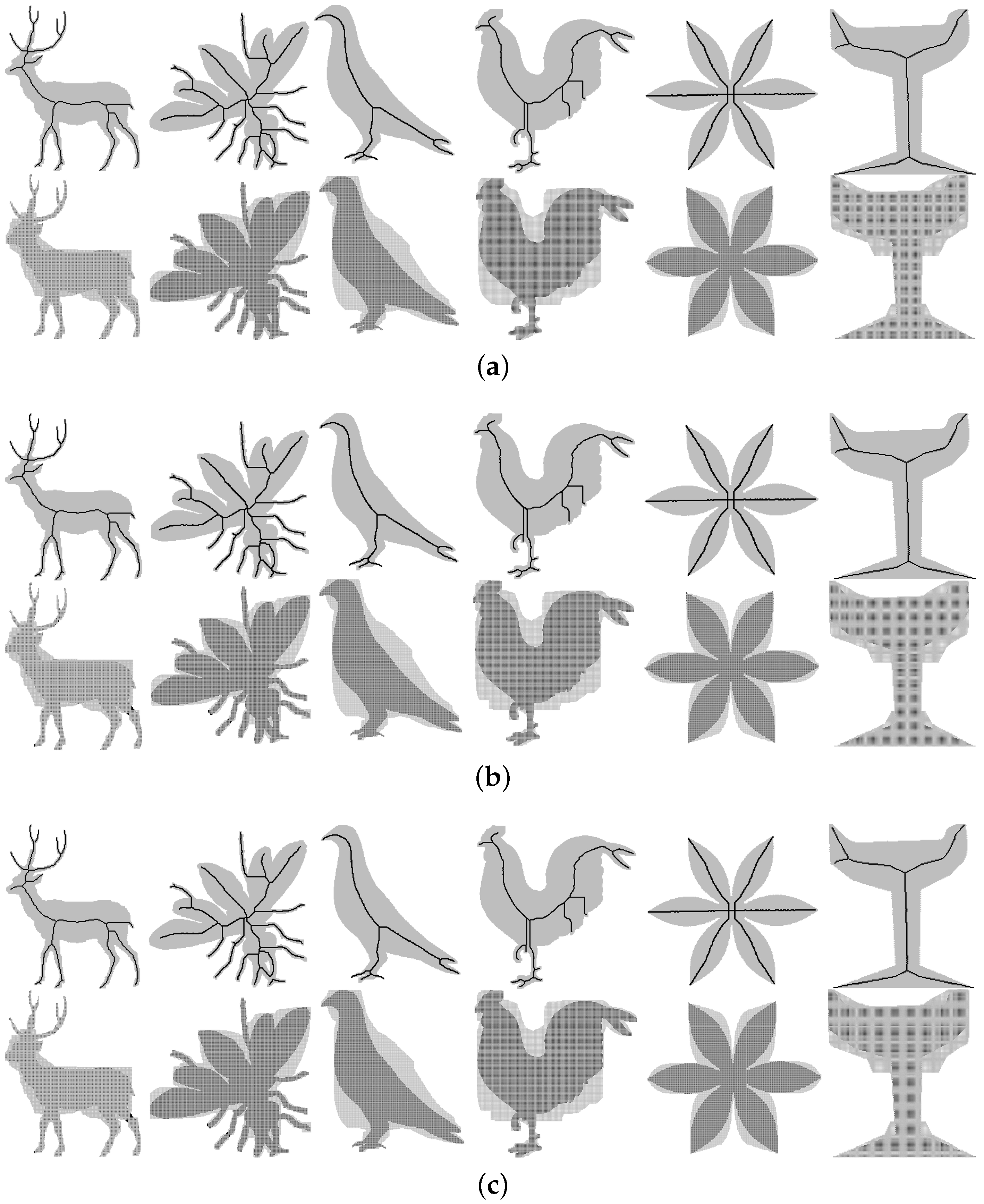
Again, the three fully-parallel thinning algorithms, CH [9], AW [16] and Rockett [20], involved in the proposed approach are used for comparisons and discussions. Figure 17 shows the obtained thinning and reconstruction results by the proposed approach without using the RHDP process. The phenomenon of over-reconstruction is very obvious. By means of the assistance of the RHDP process in the presented approach, Figure 18 demonstrates that the reconstruction results are near the original ones. In the NI and MR measurements, Table 5 reports that the average NI with the RHDP process is 28% less than that without the RHDP process, whereas Table 6 reports that the average MR with RHDP process is increased 28.4% compared to that without the RHDP process. The performances of these experiments are similar to those presented in Section 3.1. It is accordingly concluded that the feasibility of the pattern reconstruction mechanism developed for a fully-parallel thinning algorithms has been confirmed, and the bias skeleton phenomenon usually appearing in a fully-parallel thinning algorithm can be effectively reduced by involving the proposed RHDP process.
As a discussion, even the reconstruction result obtained by the proposed approach with the RHDP process is very close to the original pattern; the over-reconstructed situation is avoided; however the complete reconstruction is not easily achieved. For example, referring to Figure 15b and Figure 18, the unreconstructed portions usually appear in the convex boundaries. This phenomenon results apparently from the thinning templates and morphological structure elements adopted being of a square form, and the reconstruction result depends strongly on the thinning result. Therefore, it can be regarded as a new research direction in the near future by applying the hexagonal structure [42] to the proposed algorithms for overcoming such a phenomenon.
4. Conclusions and Future Works
In order to make a fully-parallel thinning algorithm capable of pattern reconstruction from the resultant skeleton, in this paper, an RSP-updating mechanism embedded in a thinning iteration has been presented for recording the necessary information of the thinning flag, the iteration count, as well as the reconstructable structure, thus obtaining a useful skeleton table (also the thinning result). Based on the information of the iteration count and the reconstructable structure for each skeletal pixel in the skeleton table, the pattern can be reconstructed by means of the dilating and uniting operations. In this approach, the reconstruction result is strongly related to the thinning result. If the thinning result reflects more likely the original pattern, the reconstructed pattern will be closer to the original one. For a fully-parallel thinning algorithm, there unfortunately exists a bias skeleton effect, in particular on the portions of the T-junction and L-junction. Such a biased skeleton usually results from the HDPs and will yield the over-reconstructed result using the proposed approach. Therefore, in this paper, a process of removing HDPs (RHDP) has also been presented and embedded in a thinning iteration to further reduce the bias skeleton effect. With the assistance of the RHDP process, the resultant thinning can more likely reflect the original pattern, and thus, the reconstructed pattern is closer to the original one using the proposed approach. Three well-known fully-parallel thinning algorithms investigated by means of the proposed approach with the assistance of the RHDP process confirm that 98% reconstructability (without the over-reconstructed phenomenon) can be achieved. In addition, the number of thinning iterations with the RHDP process can be reduced by about 25% compared to that without the RHDP process. Even the experimental results have confirmed the feasibility of our pattern reconstruction mechanism and RHDP process in a fully-parallel thinning algorithm; the complete (100%) reconstruction is difficult to achieve using the developed approach. The reason given is that the thinning templates and morphological structure elements adopted here are of a square form, and the reconstruction result depends strongly on the thinning result. In other words, the limit is due to the different eight-neighbor distances in a square grid as argued recently by Chen and Chao [40]. According to the equal six-neighbor distances in a hexagonal grid as reported by He and Jia [42], how to apply the hexagonal structure in the fully-parallel thinning algorithm design and the proposed approach could be a good topic and will be considered as our future works.
Acknowledgments
This work was supported in part by the Ministry of Science and Technology, Taiwan, under Grant Number MOST105-2221-E-155-063.
Author Contributions
Yung-Sheng Chen and Ming-Te Chao conceived of and designed the experiments. Ming-Te Chao performed the experiments. Yung-Sheng Chen and Ming-Te Chao analyzed the data. Yung-Sheng Chen and Ming-Te Chao wrote the paper.
Conflicts of Interest
The authors declare no conflict of interest.
Abbreviations
The following abbreviations are used in this article:
| AW | Ahmed and Ward [16] |
| CH | Chen and Hsu [9] |
| HDP | Hidden deletable point |
| MAT | Medial axis transformation |
| MR | Measurement of reconstructability |
| MSD | Measurement of skeleton deviation |
| MST | Morphological skeleton transformation |
| NI | Number of iterations |
| RHDP | Removing hidden deletable points |
| RSP | Reconstructable skeletal pixel |
| SE | Structure element |
References
- Lam, L.; Suen, C.Y. An evaluation of parallel thinning algorithms for character recognition. IEEE Trans. Pattern Anal. Mach. Intell. 1995, 17, 914–919. [Google Scholar] [CrossRef]
- Santosh, K.C.; Wendling, L. Character recognition based on non-linear multi-projection profiles measure. Front. Comput. Sci. 2015, 9, 678–690. [Google Scholar] [CrossRef]
- Ji, L.; Yi, Z.; Shang, L.; Pu, X. Binary fingerprint image thinning using template-based PCNNs. IEEE Trans. Syst. Man Cybern. 2007, 37, 1407–1413. [Google Scholar] [CrossRef]
- Xie, F.; Xu, G.; Cheng, Y.; Tian, Y. Human body and posture recognition system based on an improved thinning algorithm. IET Image Process. 2011, 5, 420–428. [Google Scholar] [CrossRef]
- Salazar-Gonzalez, A.; Kaba, D.; Li, Y.; Liu, X. Segmentation of the blood vessels and optic disk in retinal images. IEEE J. Biomed. Health Inform. 2014, 18, 1874–1886. [Google Scholar] [CrossRef] [PubMed]
- Hilditch, C.J. Linear skeletons from square cupboards. In Machine Intelligence IV; Meltzer, B., Michie, D., Eds.; American Elsevier: New York, NY, USA, 1969; pp. 403–420. [Google Scholar]
- Zhang, T.Y.; Suen, C.Y. A fast parallel algorithm for thinning digital patterns. Commun. ACM 1984, 27, 236–239. [Google Scholar] [CrossRef]
- Chen, Y.S.; Hsu, W.H. A modified fast parallel algorithm for thinning digital patterns. Pattern Recognit. Lett. 1988, 7, 99–106. [Google Scholar] [CrossRef]
- Chen, Y.S.; Hsu, W.H. A systematic approach for designing 2-subcycle and pseudo 1-subcycle parallel thinning algorithms. Pattern Recognit. 1989, 22, 267–282. [Google Scholar] [CrossRef]
- Chen, Y.S.; Hsu, W.H. A 1-subcycle parallel thinning algorithm for producing perfect 8-curves and obtaining isotropic skeleton of the L-shape pattern. In Proceedings of the IEEE Computer Society Conference on Computer Vision and Pattern Recognition, San Diego, CA, USA, 4–8 June 1989; pp. 208–215. [Google Scholar]
- Lam, L.; Lee, S.W.; Suen, C.Y. Thinning methodologies: A comprehensive survey. IEEE Trans. Pattern Anal. Mach. Intell. 1992, 14, 869–885. [Google Scholar] [CrossRef]
- Jang, B.K.; Chin, R.T. Reconstructable parallel thinning. Int. J. Pattern Recognit. Artif. Intell. 1993, 7, 1145–1181. [Google Scholar] [CrossRef]
- Hall, R. Parallel connectivity-preserving thinning algorithms. In Topological Algorithms for Digital Image Processing; Kong, T.Y., Rosenfeld, A., Eds.; Elsevier: Amsterdam, The Netherlands, 1996; pp. 145–179. [Google Scholar]
- Chen, Y.S. Hidden deletable pixel detection using vector analysis in parallel thinning to obtain bias-reduced skeletons. Comput. Vis. Image Underst. 1998, 71, 294–311. [Google Scholar] [CrossRef]
- Bernard, T.T.; Manzanera, A. Improved low complexity fully parallel thinning algorithm. In Proceedings of the IEEE International Conference on Image Analysis and Processing, Venice, Italy, 27–29 September 1999; pp. 215–220. [Google Scholar]
- Ahmed, M.; Ward, R. A rotation invariant rule-based thinning algorithm for character recognition. IEEE Trans. Pattern Anal. Mach. Intell. 2002, 24, 1672–1678. [Google Scholar] [CrossRef]
- Ranwez, V.; Soille, P. Order independent homotopic thinning for binary and grey tone anchored skeletons. Pattern Recognit. Lett. 2002, 23, 687–702. [Google Scholar] [CrossRef]
- Huang, L.; Wan, G.; Liu, C. An improved parallel thinning algorithm. In Proceedings of the International Conference on Document Analysis and Recognition, Edinburgh, UK, 3–6 August 2003; pp. 780–783. [Google Scholar]
- Patil, P.M.; Suralkar, S.R.; Sheikh, F.B. Rotation invariant thinning algorithm to detect ridge bifurcations for fingerprint identification. In Proceedings of the IEEE International Conference on Tools with Artificial Intelligence, Hong Kong, China, 14–16 November 2005; pp. 634–641. [Google Scholar]
- Rockett, P.I. An improved rotation-invariant thinning algorithm. IEEE Trans. Pattern Anal. Mach. Intell. 2005, 27, 1671–1674. [Google Scholar] [CrossRef] [PubMed]
- Bertrand, G.; Couprie, M. Two-dimensional parallel thinning algorithms based on critical kernels. J. Math. Imaging Vis. 2008, 31, 35–56. [Google Scholar] [CrossRef]
- Németh, G.; Kardos, P.; Palágyi, K. 2D parallel thinning and shrinking based on sufficient conditions for topology preservation. Acta Cybern. 2011, 20, 125–144. [Google Scholar]
- Chen, W.; Sui, L.; Xu, Z.; Lang, Y. Improved Zhang-Suen thinning algorithm in binary line drawing applications. In Proceedings of the International Conference on Systems and Informatics, Yantai, China, 19–20 May 2012; pp. 1947–1950. [Google Scholar]
- Tarabek, P. A robust parallel thinning algorithm for pattern recognition. In Proceedings of the IEEE International Symposium on Applied Computational Intelligence and Informatics (SACI), Timisoara, Romania, 24–26 May 2012; pp. 75–79. [Google Scholar]
- Kwon, J.S. Improved parallel thinning algorithm to obtain unit-width skeleton. Int. J. Multimed. Its Appl. 2013, 5, 1–14. [Google Scholar] [CrossRef]
- Paágyi, K. Equivalent sequential and parallel reductions in arbitrary binary pictures. Int. J. Pattern Recognit. Artif. Intell. 2014, 28, 1460009. [Google Scholar]
- Blum, H. A transformation for extracting new descriptors of shape. In Models for the Perception of Speech and Visual Form; Wathen-Dunn, W., Ed.; MIT Press: Cambridge, MA, USA, 1967; pp. 362–380. [Google Scholar]
- Montanari, U. Continuous skeletons from digitized. J. ACM 1969, 16, 534–549. [Google Scholar] [CrossRef]
- Blum, H.; Nagel, R.N. Shape description using weighted symmetric axis features. Pattern Recognit. 1978, 10, 167–180. [Google Scholar] [CrossRef]
- Peleg, S.; Rosenfeld, A. A min-max medial axis transformation. IEEE Trans. Pattern Anal. Mach. Intell. 1981, 3, 208–210. [Google Scholar] [CrossRef] [PubMed]
- Chen, Y.S.; Hsu, W.H. MATNET: A neural network for medial axis transformation. J. Chin. Inst. Eng. 1993, 16, 757–771. [Google Scholar] [CrossRef]
- Shih, F.Y.; Pu, C.C. A skeletonization algorithm by maxima tracking on Euclidean distance transform. Pattern Recognit. 1995, 28, 331–341. [Google Scholar] [CrossRef]
- Chang, S. Extracting skeletons from distance maps. Int. J.Comput. Sci. Netw. Secur. 2007, 7, 213–219. [Google Scholar]
- Yan, T.Q.; Zhou, C.X. A continuous skeletonization method based on distance transform. Commun. Comput. Inf. Sci. 2012, 304, 251–258. [Google Scholar]
- Saha, P.K.; Borgefors, G.; di Baja, G.S. A survey on skeletonization algorithms and their applications. Pattern Recognit. Lett. 2016, 76, 3–12. [Google Scholar] [CrossRef]
- Saha, P.K.; Borgefors, G.; di Baja, G.S. Skeletonization: Theory, Methods and Applications, 1st ed.; Academic Press, Elsevier Ltd.: Cambridge, MA, USA, 2017. [Google Scholar]
- Bertrand, G. On critical kernels. C. R. Math. 2007, 345, 363–367. [Google Scholar] [CrossRef]
- Rosenfeld, A.; Kak, A.C. Digital Picture Processing, 2nd ed.; Academic Press: New York, NY, USA, 1982; Volume 2. [Google Scholar]
- Gonzalez, R.C.; Woods, R.E. Digital Image Processing, 2nd ed.; Prentice-Hall Inc.: Upper Saddle River, NJ, USA, 2002. [Google Scholar]
- Chen, Y.S.; Chao, M.T. MAT based thinning for line patterns. Int. J. Pattern Recognit. Artif. Intell. 2016, 30, 1654001. [Google Scholar] [CrossRef]
- Latecki, L.J.; Lakamper, R.; Eckhardt, U. Shape descriptors for non-rigid shapes with a single closed contour. In Proceedings of the International Conference on Computer Vision and Pattern Recognition, Hilton Head Island, SC, USA, 13–15 June 2000; pp. 424–429. [Google Scholar]
- He, X.; Jia, W. Hexagonal structure for intelligent vision. In Proceedings of the International Conference on Information and Communication Technologies, Karachi, Pakistan, 27–28 August 2005; pp. 52–64. [Google Scholar]
Figure 1.
Illustration of Jang and Chin’s MST-based reconstructable parallel thinning. (a) Feature pixels obtained from the MST, (b) the final skeleton containing reduced feature pixels, feature pixels and the unit-width pixels to ensure pattern reconstruction, as well as (c) the reconstructed pattern.
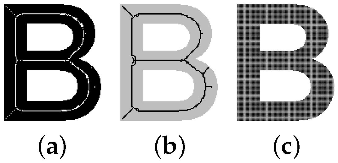
Figure 2.
Flowchart of the proposed approach for digital pattern (a) thinning and (b) reconstruction.
Figure 2.
Flowchart of the proposed approach for digital pattern (a) thinning and (b) reconstruction.
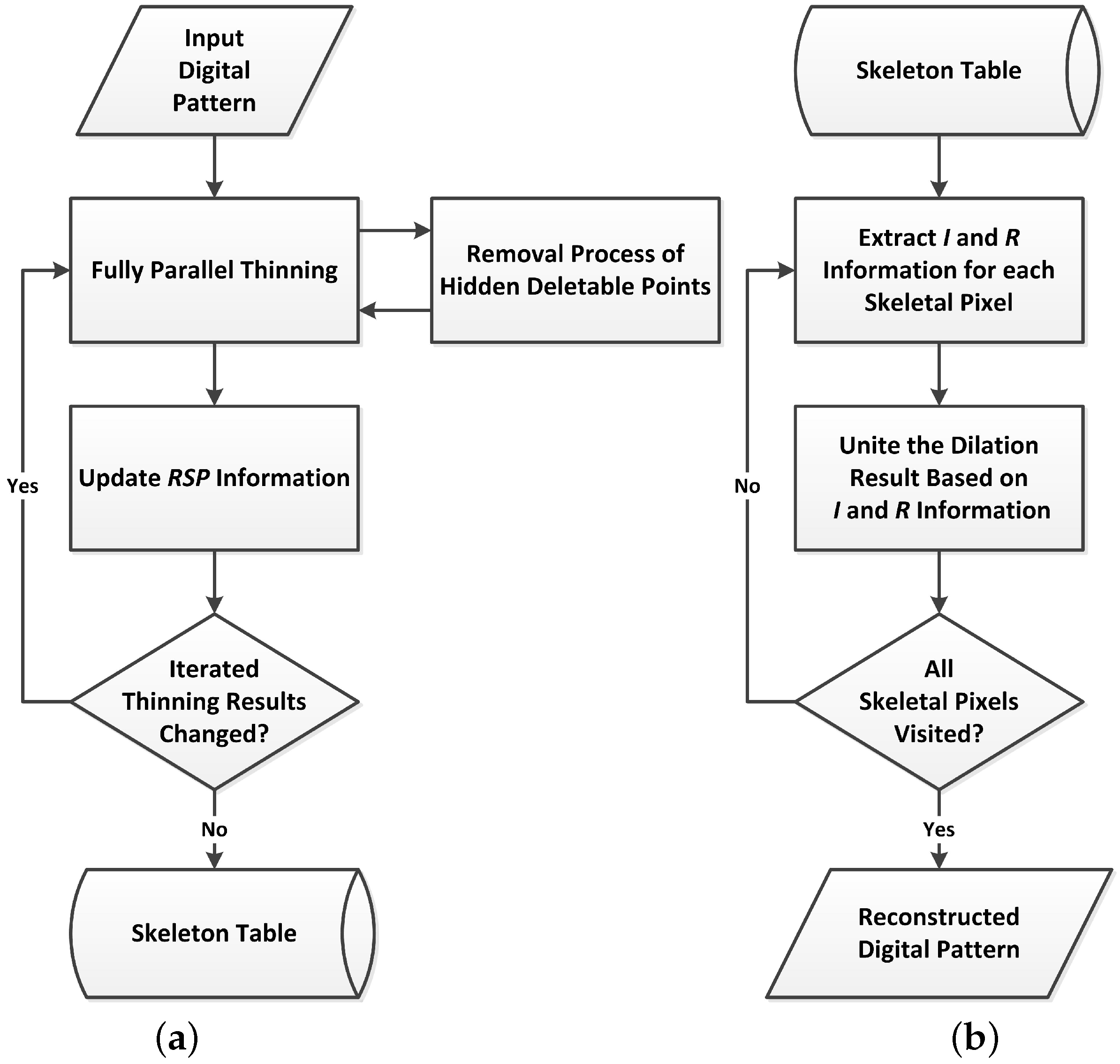
Figure 3.
Definition of eight neighbors for a pixel P.
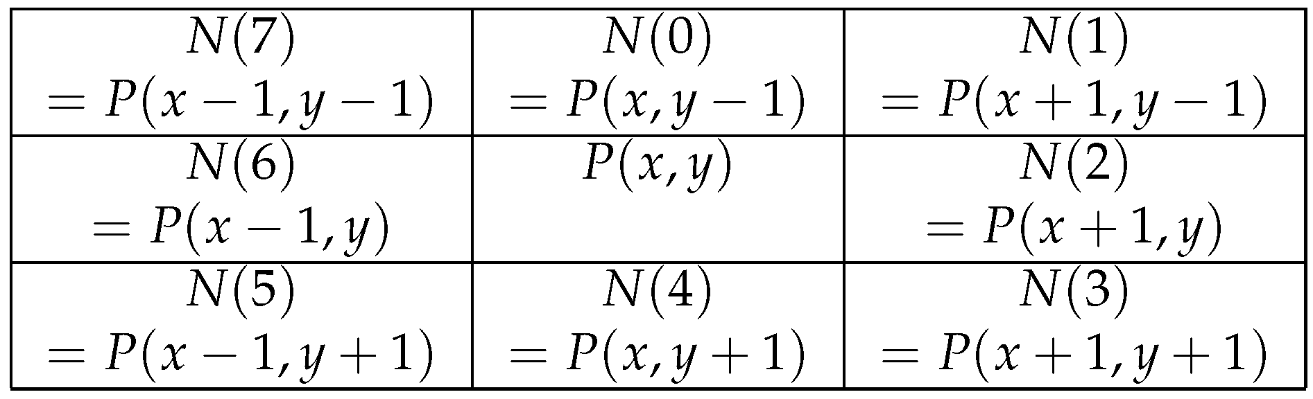
Figure 4.
Definition of 16-bit data format for a reconstructable skeletal pixel (RSP)-pixel.

Figure 5.
(a) Input digital pattern. The thinning results at the 1st, 2nd and 3rd iteration are shown in (b–d), respectively. The numbers in (e) illustrate the points removed at the related thinning iteration.
Figure 5.
(a) Input digital pattern. The thinning results at the 1st, 2nd and 3rd iteration are shown in (b–d), respectively. The numbers in (e) illustrate the points removed at the related thinning iteration.

Figure 6.
Illustrations of a 1-pixel in (b) and its eight neighbors confined by a dotted square. The current iteration count for thinning is 3. According to the Equation (4), (c) presents the C-value calculated for the three 1-neighbor , , and in (a) and that calculated for the 1-pixel in (b).
Figure 6.
Illustrations of a 1-pixel in (b) and its eight neighbors confined by a dotted square. The current iteration count for thinning is 3. According to the Equation (4), (c) presents the C-value calculated for the three 1-neighbor , , and in (a) and that calculated for the 1-pixel in (b).
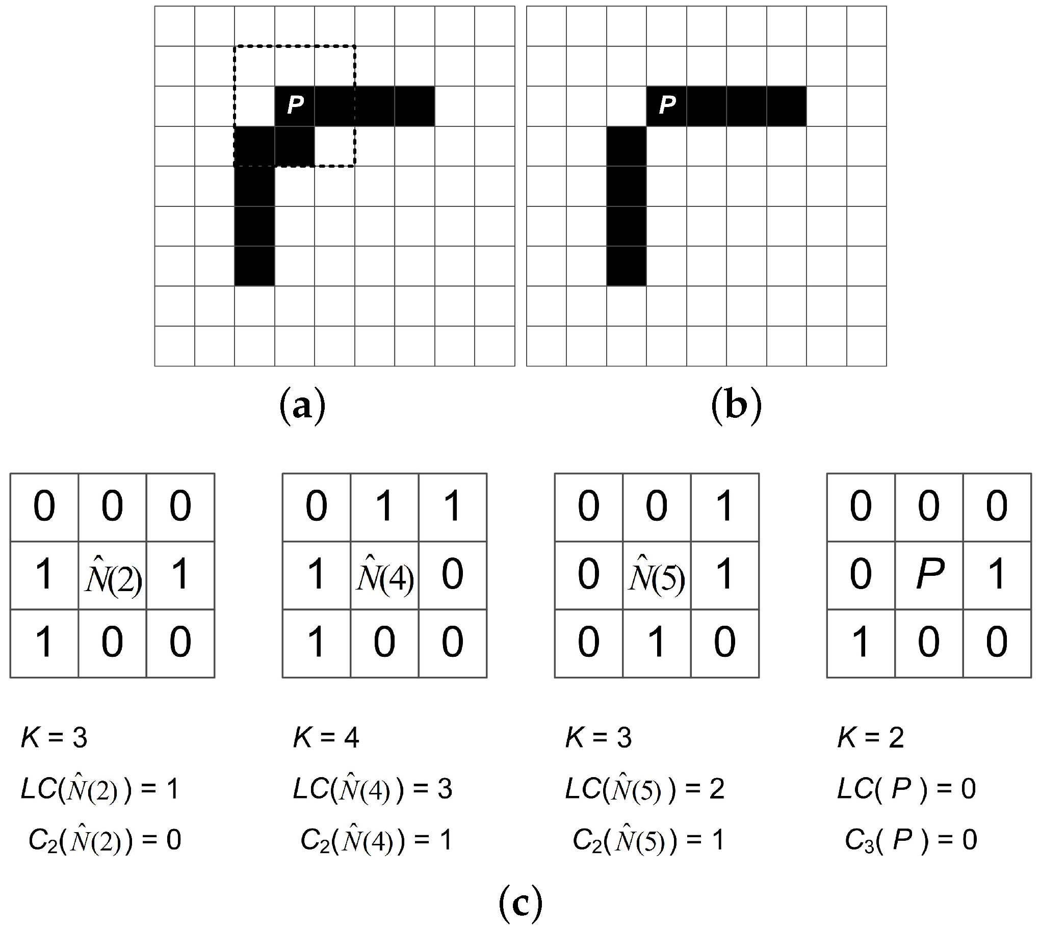
Figure 7.
Illustrations of RSP updating from to . (a) Null RSP matrix initially. That is, the RSP information is set to be (0 0 0) in decimal or (0 000000 00000000) in binary. (b) Thinning result , where the original pattern is regarded as and confined by a dotted line for reference. (b–h) show the updated RSP information for each 1-pixel P satisfying in , where the reconstructable information is numbered. (i) The updated RSP pixel is denoted with a gray square.

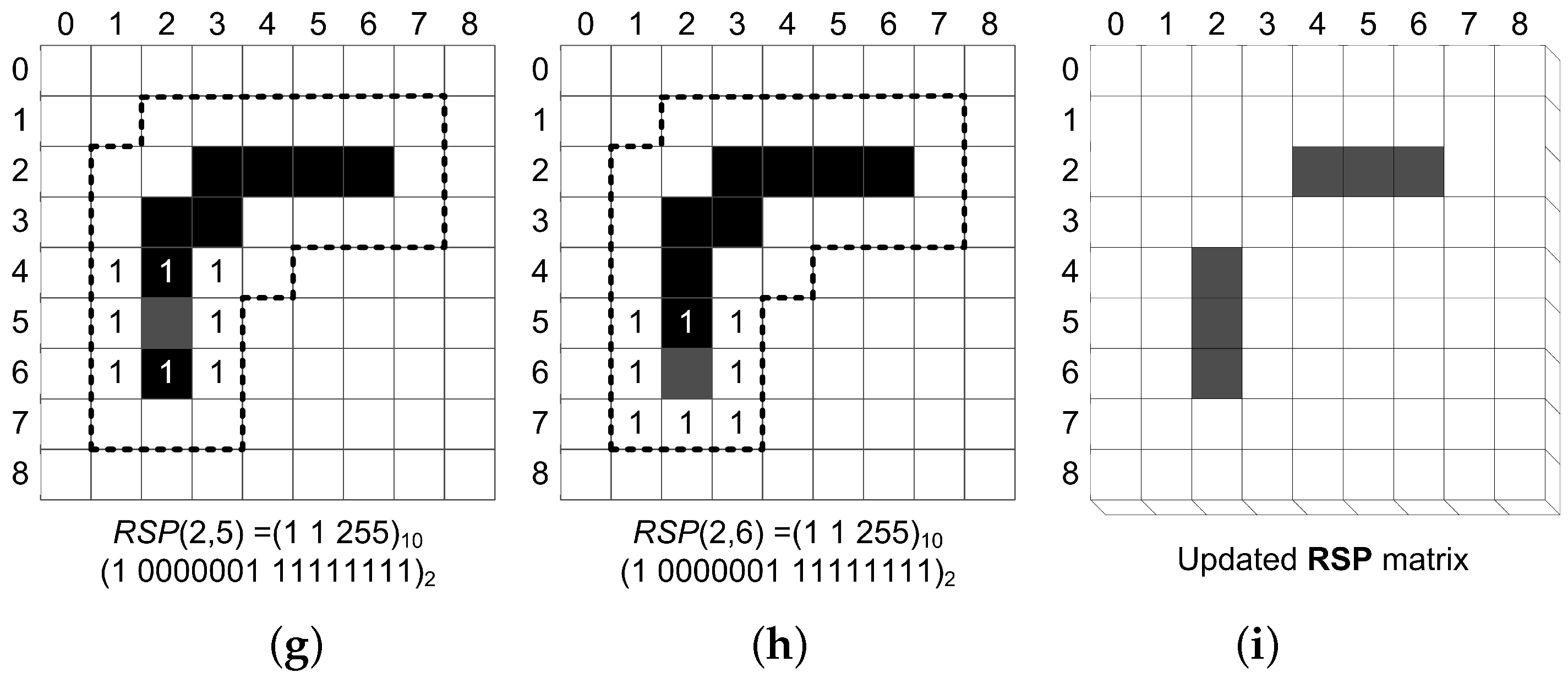
Figure 8.
Illustrations of RSP updating from to . (a) The RSP matrix at , where six skeletal pixels have been identified. (b) Thinning result . (c,d) show respectively the updated RSP information for the 1-pixel (2, 3) and (3, 2) having zero C value in . (e) The updated RSP pixel is denoted with a gray square. The RSP matrix can be decomposed into F, I and R matrices, as shown in (f,g,h), respectively.

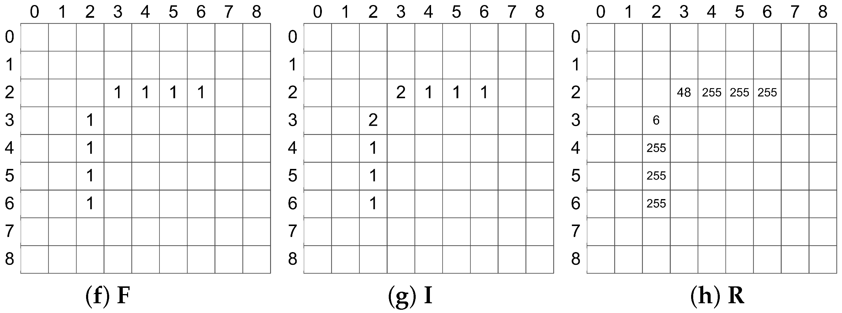
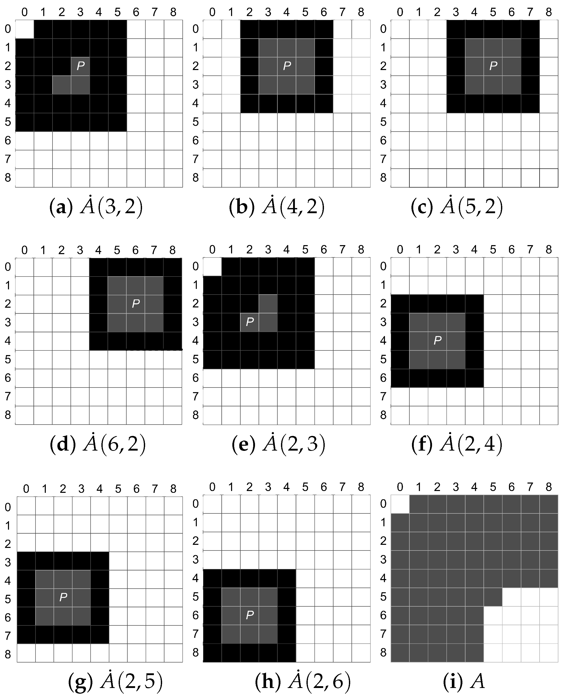
Figure 9.
Illustrations of pattern reconstruction from the skeleton table. Reconstructed partial pattern from (a) , (b) , (c) , (d) , (e) , (f) , (g) and (h) . Here, the reconstructable information 1-neighbor is displayed by a gray square. (i) shows the final reconstructed pattern A with the union of these partial patterns ()s.

Figure 10.
(a–d) The original thinning results at the 1st, 2nd, 3rd and 4th iteration by means of the fully-parallel thinning without the assistance of RHDP process. (e) Gray squares show the reconstructed pattern with our approach. It is obviously over-reconstructed due to the HDP effect.
Figure 10.
(a–d) The original thinning results at the 1st, 2nd, 3rd and 4th iteration by means of the fully-parallel thinning without the assistance of RHDP process. (e) Gray squares show the reconstructed pattern with our approach. It is obviously over-reconstructed due to the HDP effect.

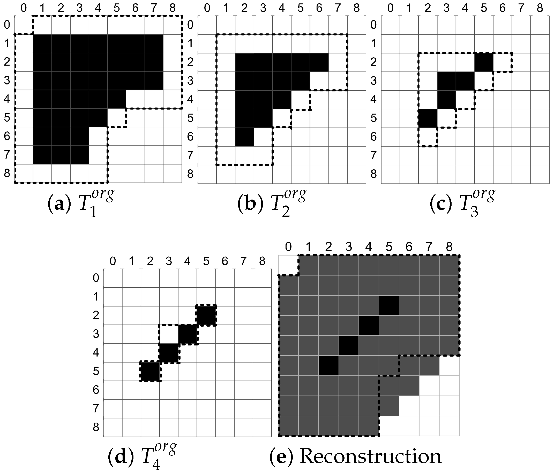
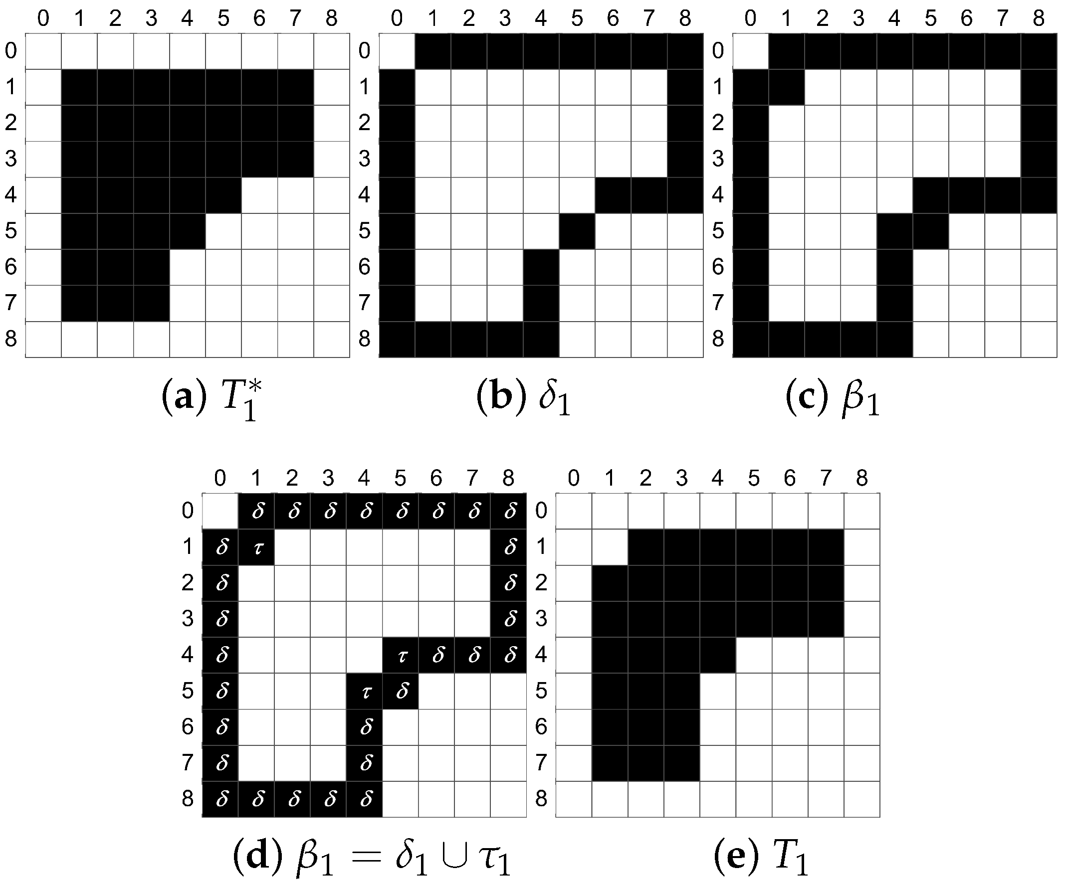
Figure 11.
Illustrations of transforming into . With in Figure 5a, (a) shows the next thinning result purely obtained by Chen and Hsu’s algorithm [9]; (b,c) shows the corresponding and . To clarify, let the - and -points be marked on the -image, as shown in (d). According to the Step 4 of RHDP, the three points, (1, 1), (5, 4) and (4, 5), are HDPs. They can be further removed from , and the new thinning result is thus obtained as shown in (e).

Figure 12.
The thinning result obtained (a) without and (b) with the assistance of RHDP. (c,d) show the corresponding reconstruction result, where the original pattern pixels and the reconstructed pixels are marked by “black region squares” and “gray frame squares” respectively.
Figure 12.
The thinning result obtained (a) without and (b) with the assistance of RHDP. (c,d) show the corresponding reconstruction result, where the original pattern pixels and the reconstructed pixels are marked by “black region squares” and “gray frame squares” respectively.
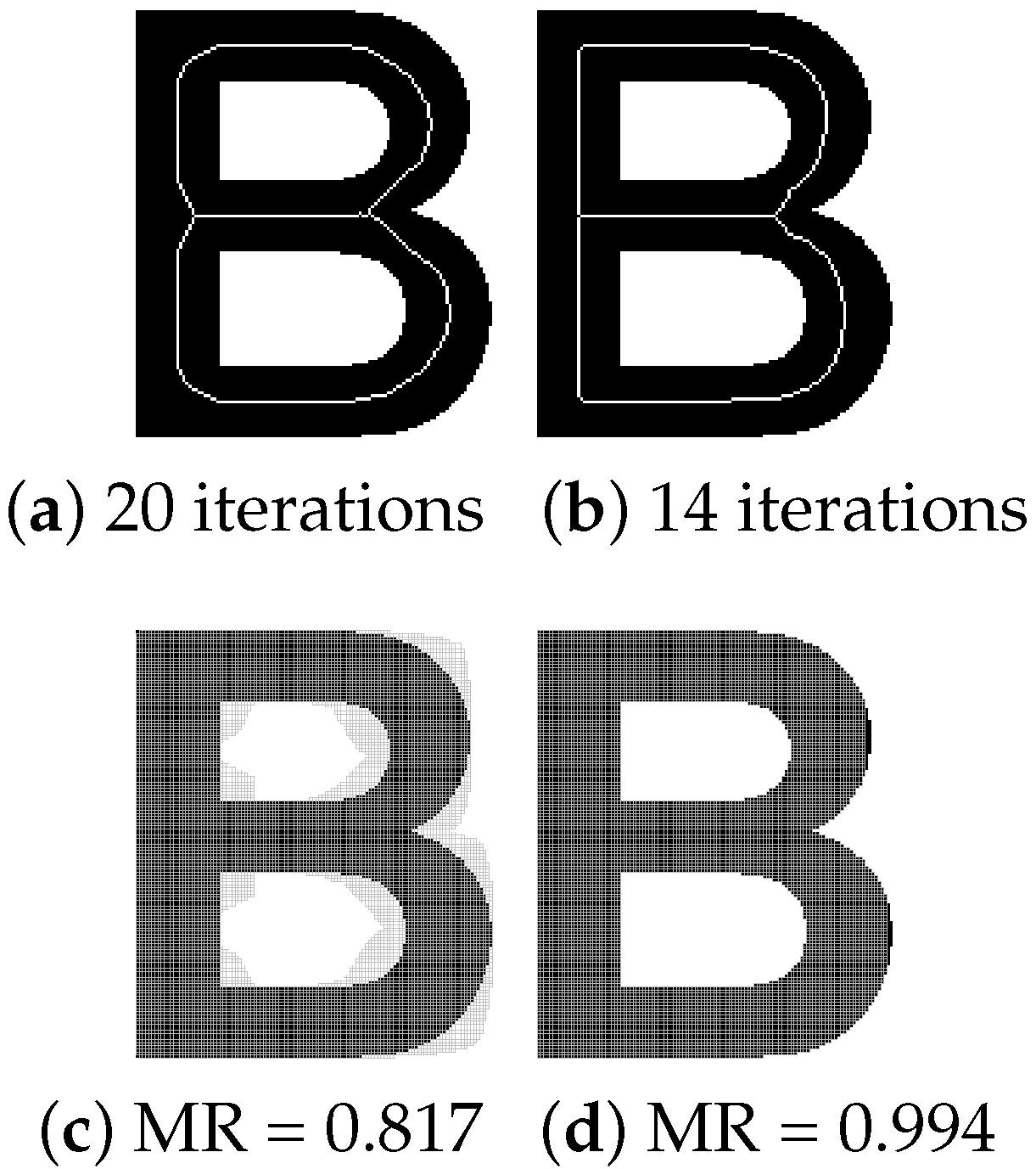
Figure 13.
(a) Seven unit-width letters used as ground truths for MSD measurements. (b) Thickened digital patterns from (a) used for the investigations of MR, NI and MSD.
Figure 13.
(a) Seven unit-width letters used as ground truths for MSD measurements. (b) Thickened digital patterns from (a) used for the investigations of MR, NI and MSD.
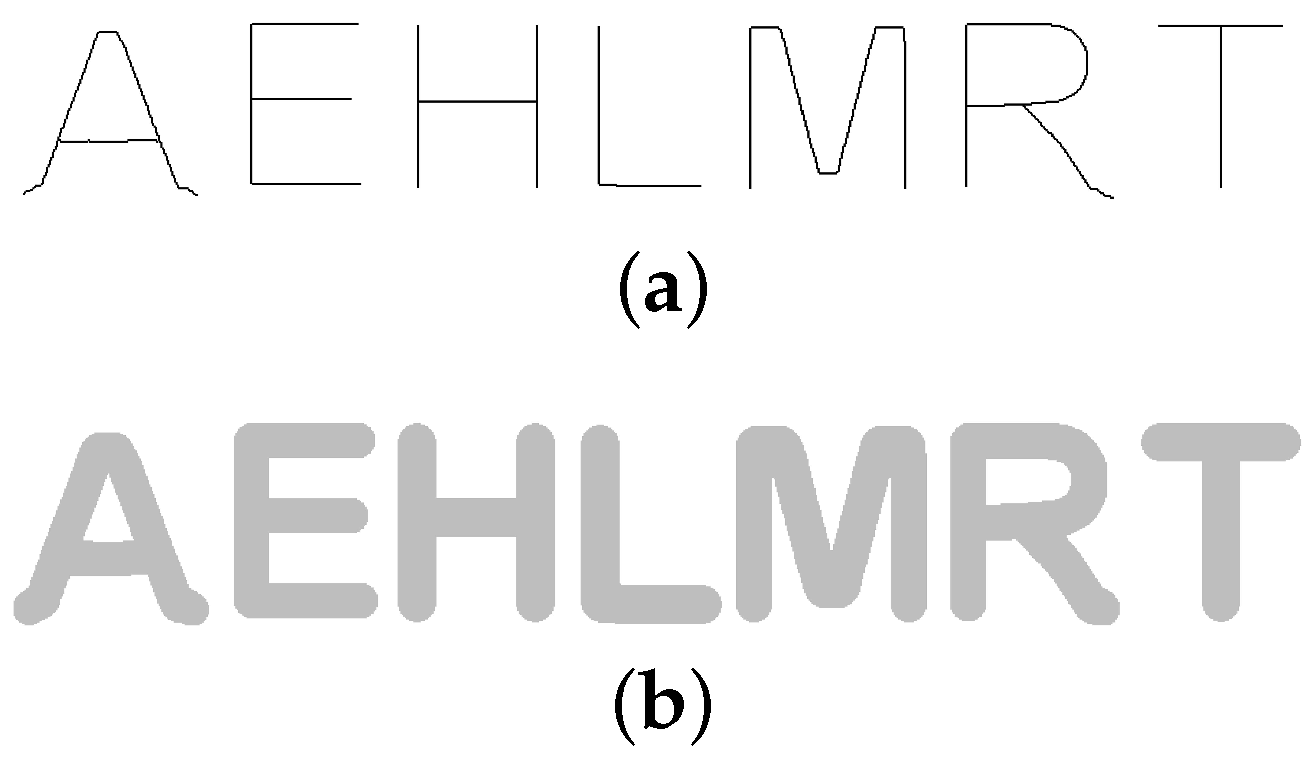
Figure 14.
Thinning results (a) without and (b) with the RHDP process are obtained by the three fully-parallel thinning algorithms involved in the proposed approach for comparisons. The biased skeletons of (b) are much less than those of (a).
Figure 14.
Thinning results (a) without and (b) with the RHDP process are obtained by the three fully-parallel thinning algorithms involved in the proposed approach for comparisons. The biased skeletons of (b) are much less than those of (a).

Figure 15.
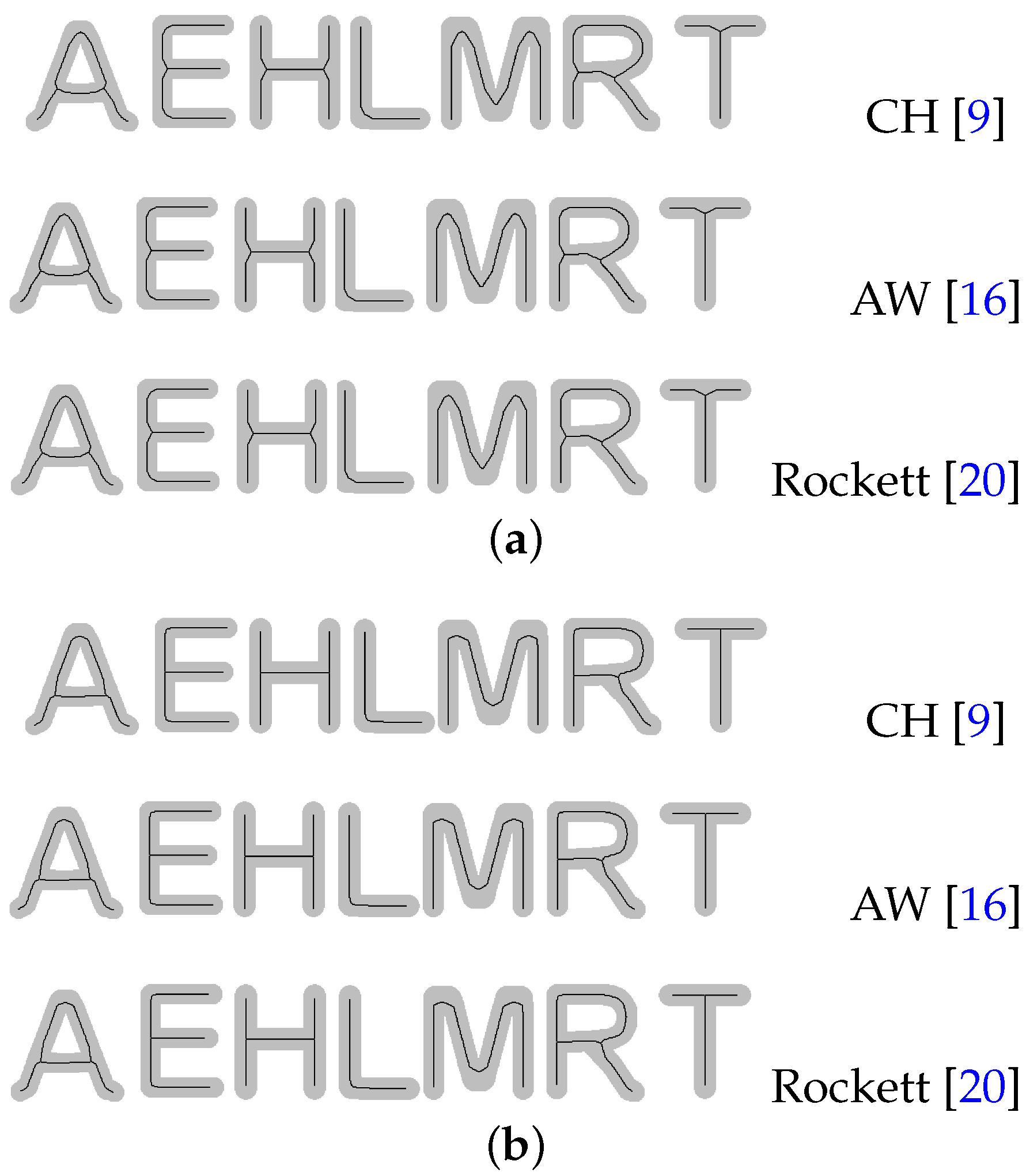
Reconstruction results (a) without and (b) with the RHDP process are obtained by the three fully-parallel thinning algorithms involved in the proposed approach for comparisons. The reconstruction results of (a) are over-reconstructed, whereas those of (b) are closer to the originals.
Figure 15.
Reconstruction results (a) without and (b) with the RHDP process are obtained by the three fully-parallel thinning algorithms involved in the proposed approach for comparisons. The reconstruction results of (a) are over-reconstructed, whereas those of (b) are closer to the originals.

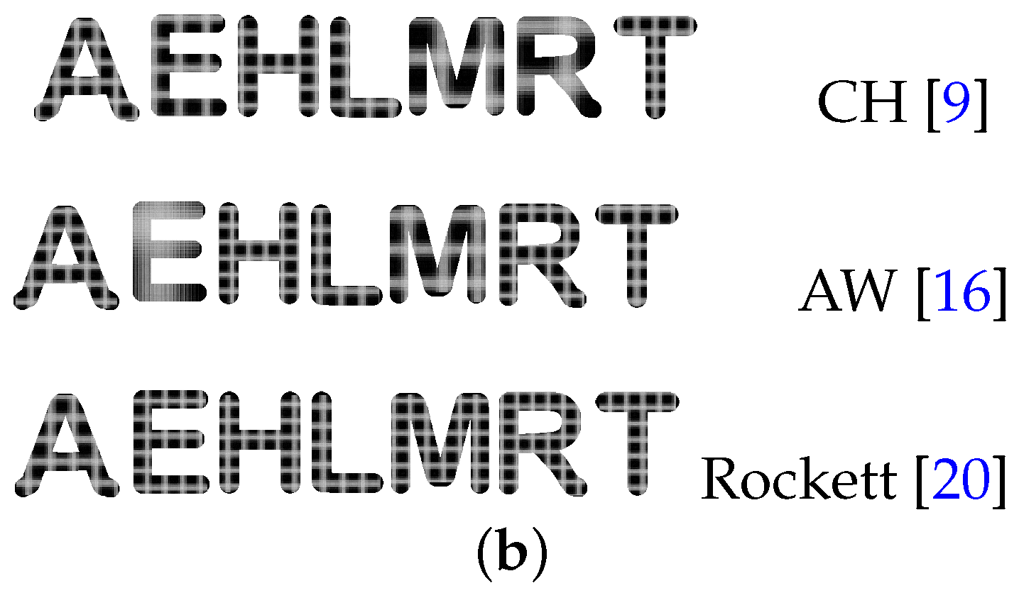
Figure 16.
(a) Thinning results and (b) reconstruction results of some patterns from the MPEG7 CE-Shape-1 dataset are obtained by Jang and Chin’s MST-based reconstructable parallel thinning algorithm. To completely reconstruct the whole pattern, the feature points obtained by MST are retained in the thinning process, and thus, many unwanted branches are yielded in the resultant skeletons.

Figure 17.
Results of some patterns from the MPEG7 CE-Shape-1 dataset are obtained by the three fully-parallel thinning algorithms involved in the proposed approach without the RHDP process for comparisons. Here, the thinning and reconstruction results are placed on the first and second row, respectively. The phenomenon of over-reconstruction is very obvious. (a) CH [9]; (b) AW [16]; (c) Rockett [20].

Figure 18.
Results of some patterns from the MPEG7 CE-Shape-1 dataset are obtained by the three fully-parallel thinning algorithms involved in the proposed approach with the RHDP process for comparisons. Here, the thinning and reconstruction results are placed at the first and second row, respectively. The reconstruction results are near the original ones. (a) CH [9]; (b) AW [16]; (c) Rockett [20].

Table 1.
The final 8 skeletal pixels, recorded with their coordinates, I and R information, form a skeleton table.
Table 1.
The final 8 skeletal pixels, recorded with their coordinates, I and R information, form a skeleton table.
| Skeletal Pixels | Coordinates | I | R |
|---|---|---|---|
| 1 | (3, 2) | 2 | 48 |
| 2 | (4, 2) | 1 | 255 |
| 3 | (5, 2) | 1 | 255 |
| 4 | (6, 2) | 1 | 255 |
| 5 | (2, 3) | 2 | 6 |
| 6 | (2, 4) | 1 | 255 |
| 7 | (2, 5) | 1 | 255 |
| 8 | (2, 6) | 1 | 255 |
Table 2.
NI measurements for the results given in Figure 14 by applying the presented approach with three fully-parallel thinning algorithms. The average NI with the RHDP process is 27% less than that without the RHDP process.
Table 2.
NI measurements for the results given in Figure 14 by applying the presented approach with three fully-parallel thinning algorithms. The average NI with the RHDP process is 27% less than that without the RHDP process.
| Without RHDP | With RHDP | ||||||
|---|---|---|---|---|---|---|---|
| Pattern | CH [9] | AW [16] | Rockett [20] | CH [9] | AW [16] | Rockett [20] | |
| “A” | 20 | 20 | 20 | 15 | 15 | 15 | |
| “E” | 19 | 19 | 19 | 13 | 13 | 13 | |
| “H” | 21 | 21 | 21 | 14 | 14 | 14 | |
| “L” | 19 | 19 | 19 | 14 | 14 | 14 | |
| “M” | 21 | 21 | 21 | 18 | 18 | 18 | |
| “R” | 22 | 22 | 22 | 16 | 16 | 16 | |
| “T” | 21 | 21 | 21 | 14 | 14 | 14 | |
| Average | 20.4 | 20.4 | 20.4 | 14.9 | 14.9 | 14.9 | |
Table 3.
MSD measurements for the results given in Figure 14 by applying the presented approach with three fully-parallel thinning algorithms. The average MSD with the RHDP process is 42% less than that without the RHDP process.
Table 3.
MSD measurements for the results given in Figure 14 by applying the presented approach with three fully-parallel thinning algorithms. The average MSD with the RHDP process is 42% less than that without the RHDP process.
| Without RHDP | With RHDP | ||||||
|---|---|---|---|---|---|---|---|
| Pattern | CH [9] | AW [16] | Rockett [20] | CH [9] | AW [16] | Rockett [20] | |
| “A” | 295.1 | 328.3 | 288.1 | 221.9 | 218.1 | 218.1 | |
| “E” | 116 | 124 | 116 | 24 | 22 | 22 | |
| “H” | 120 | 120 | 120 | 12 | 12 | 12 | |
| “L” | 40 | 40 | 40 | 25 | 23 | 23 | |
| “M” | 469.9 | 512.6 | 469.9 | 342.4 | 348.4 | 348.4 | |
| “R” | 238.8 | 263.6 | 240.9 | 162.8 | 164.5 | 164.5 | |
| “T” | 60 | 60 | 60 | 6 | 6 | 6 | |
| Average | 191.4 | 206.9 | 190.7 | 113.4 | 113.4 | 113.4 | |
Table 4.
MR measurements for the results given in Figure 15 by applying the presented pattern reconstruction approach with three fully-parallel thinning algorithms. The average MR with the RHDP process is increased 12.5% compared to that without the RHDP process.
Table 4.
MR measurements for the results given in Figure 15 by applying the presented pattern reconstruction approach with three fully-parallel thinning algorithms. The average MR with the RHDP process is increased 12.5% compared to that without the RHDP process.
| Without RHDP | With RHDP | ||||||
|---|---|---|---|---|---|---|---|
| Pattern | CH [9] | AW [16] | Rockett [20] | CH [9] | AW [16] | Rockett [20] | |
| “A” | 0.695 | 0.700 | 0.700 | 0.982 | 0.982 | 0.982 | |
| “E” | 0.927 | 0.927 | 0.927 | 0.988 | 0.988 | 0.988 | |
| “H” | 0.900 | 0.900 | 0.900 | 0.981 | 0.981 | 0.981 | |
| “L” | 0.931 | 0.931 | 0.931 | 0.975 | 0.975 | 0.975 | |
| “M” | 0.878 | 0.878 | 0.878 | 0.976 | 0.976 | 0.976 | |
| “R” | 0.751 | 0.754 | 0.754 | 0.992 | 0.992 | 0.992 | |
| “T” | 0.911 | 0.911 | 0.911 | 0.974 | 0.974 | 0.974 | |
| Average | 0.856 | 0.857 | 0.857 | 0.981 | 0.981 | 0.981 | |
Table 5.
NI measurements for the thinning results given in Figure 17 and Figure 18 by applying the presented approach with three fully-parallel thinning algorithms. The average NI with the RHDP process is 28% less than that without the RHDP process.
| Without RHDP | With RHDP | ||||||
|---|---|---|---|---|---|---|---|
| Pattern | CH [9] | AW [16] | Rockett [20] | CH [9] | AW [16] | Rockett [20] | |
| Deer | 31 | 31 | 31 | 25 | 25 | 25 | |
| Fly | 39 | 39 | 39 | 31 | 31 | 31 | |
| Bird | 52 | 52 | 52 | 30 | 29 | 29 | |
| Chicken | 62 | 61 | 61 | 44 | 44 | 44 | |
| Device | 26 | 25 | 25 | 21 | 21 | 21 | |
| Glass | 36 | 36 | 36 | 26 | 26 | 26 | |
| Average | 41.0 | 40.7 | 40.7 | 29.5 | 29.3 | 29.3 | |
Table 6.
MR measurements for the reconstruction results given in Figure 17 and Figure 18 by applying the presented pattern reconstruction approach with three fully-parallel thinning algorithms. The average MR with the RHDP process is increased 28.4% compared to that without the RHDP process.
| Without RHDP | With RHDP | ||||||
|---|---|---|---|---|---|---|---|
| Pattern | CH [9] | AW [16] | Rockett [20] | CH [9] | AW [16] | Rockett [20] | |
| Deer | 0.751 | 0.759 | 0.759 | 0.981 | 0.981 | 0.981 | |
| Fly | 0.772 | 0.773 | 0.773 | 0.981 | 0.979 | 0.979 | |
| Bird | 0.541 | 0.543 | 0.543 | 0.989 | 0.989 | 0.989 | |
| Chicken | 0.664 | 0.670 | 0.670 | 0.978 | 0.978 | 0.978 | |
| Device | 0.712 | 0.713 | 0.713 | 0.988 | 0.988 | 0.988 | |
| Glass | 0.755 | 0.755 | 0.755 | 0.994 | 0.994 | 0.994 | |
| Average | 0.699 | 0.702 | 0.702 | 0.985 | 0.985 | 0.985 | |
© 2017 by the authors. Licensee MDPI, Basel, Switzerland. This article is an open access article distributed under the terms and conditions of the Creative Commons Attribution (CC BY) license (http://creativecommons.org/licenses/by/4.0/).
Share and Cite
MDPI and ACS Style
Chen, Y.-S.; Chao, M.-T. Pattern Reconstructability in Fully Parallel Thinning. J. Imaging 2017, 3, 29. https://doi.org/10.3390/jimaging3030029
AMA Style
Chen Y-S, Chao M-T. Pattern Reconstructability in Fully Parallel Thinning. Journal of Imaging. 2017; 3(3):29. https://doi.org/10.3390/jimaging3030029
Chicago/Turabian StyleChen, Yung-Sheng, and Ming-Te Chao. 2017. "Pattern Reconstructability in Fully Parallel Thinning" Journal of Imaging 3, no. 3: 29. https://doi.org/10.3390/jimaging3030029
Note that from the first issue of 2016, this journal uses article numbers instead of page numbers. See further details here.