This section evaluates the proposed method from both quantitative and qualitative perspectives. The evaluation metrics and their applicable data types are first introduced. The recovered vignette fields, corrected remote sensing images, statistical comparisons, and star image results are then analyzed to assess correction accuracy, spatial uniformity, radiometric consistency, and the respective contributions of low-rank modeling and polynomial fitting.
3.2. Analysis of Ablation Results
This section further analyzes the role of polynomial fitting after low-rank decomposition and provides a quantitative comparison of different correction strategies. The purpose is to clarify why low-rank decomposition alone is insufficient to recover a physically plausible vignette field, and how polynomial fitting improves the spatial smoothness and low-frequency consistency of the estimated field. In addition to the ablation comparison among the low-rank-only, polynomial-only, and full methods, representative external baseline methods are also included to evaluate the competitiveness of the proposed method under the same datasets and metrics.
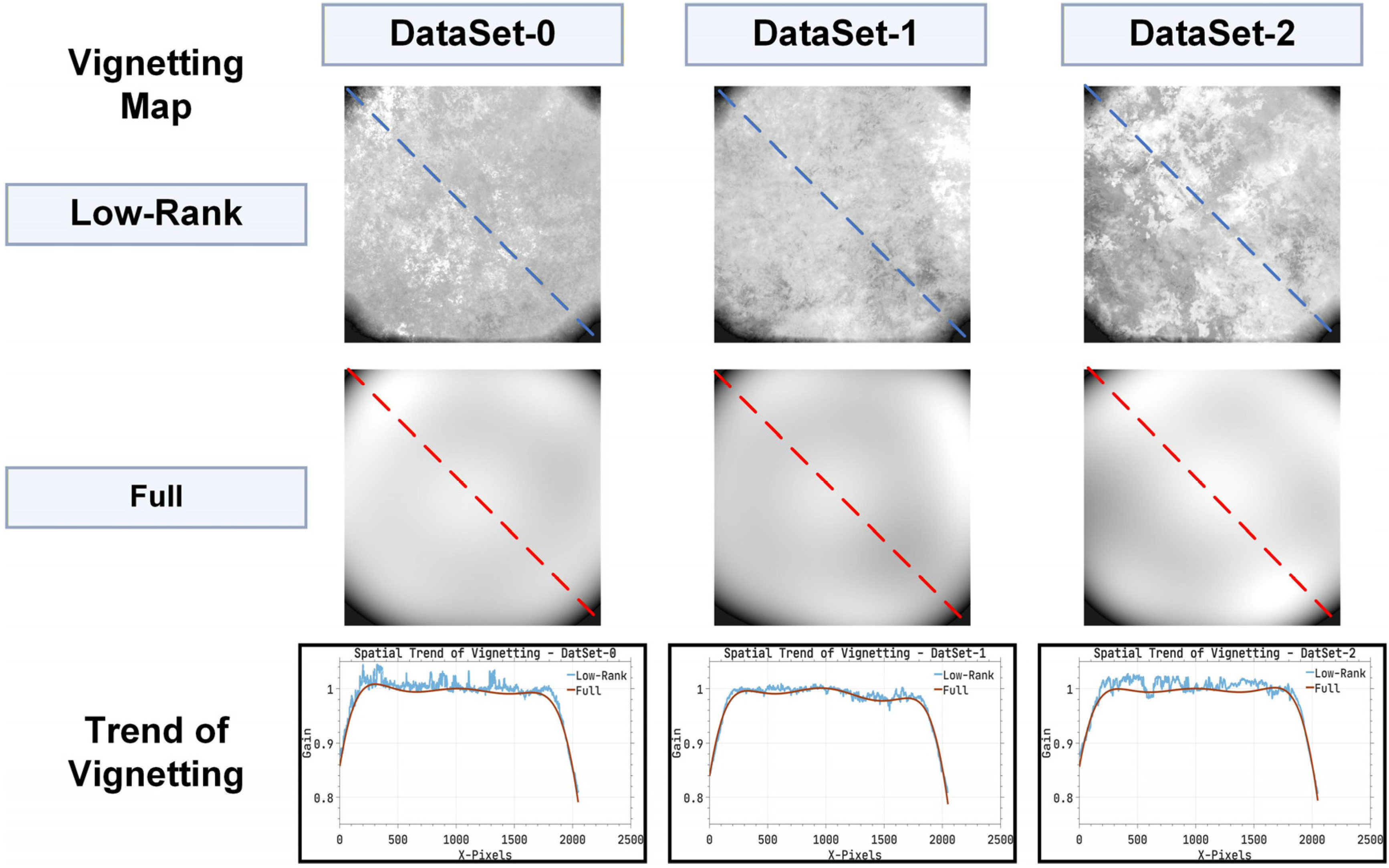
As shown in
Figure 2, the vignette field obtained after low-rank decomposition mainly characterizes the common structural component in multiple images. However, the result may still be affected by local residual textures and non-smooth disturbances, and is therefore insufficient to fully represent the vignette distribution of the actual imaging system. After further polynomial fitting, the obtained vignette field better conforms to the physical characteristics of the true vignette field.
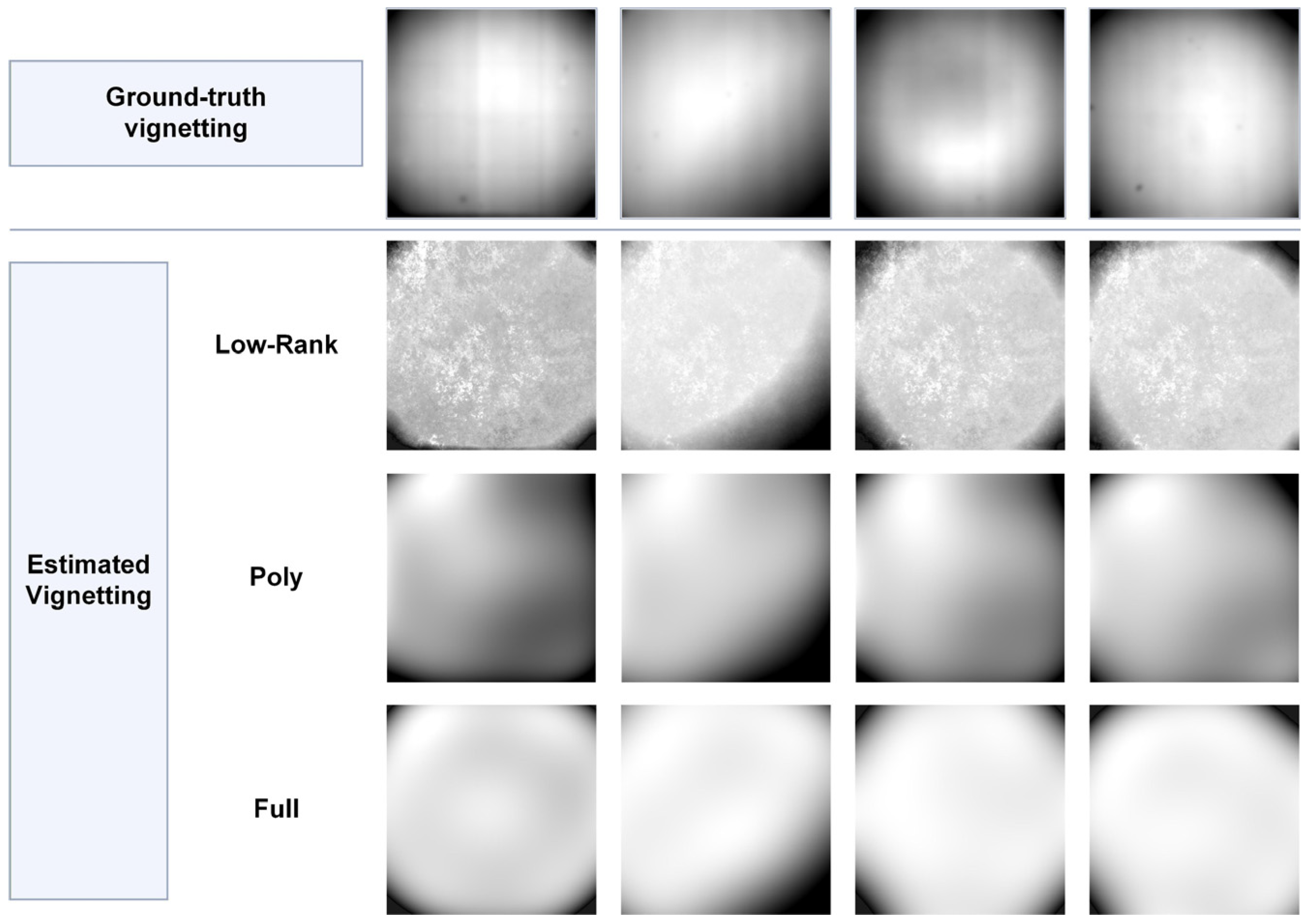
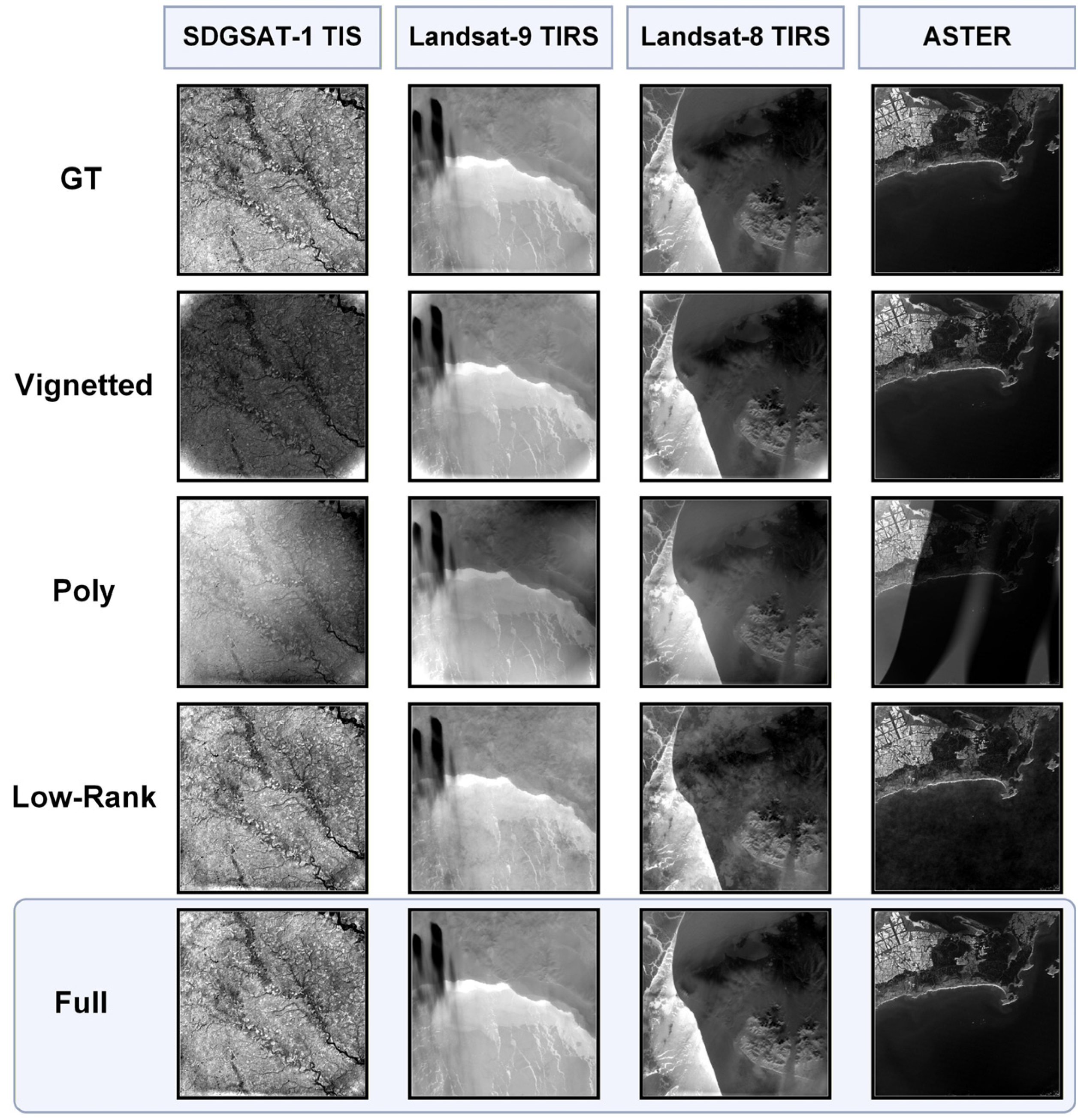
As shown in
Figure 3 and
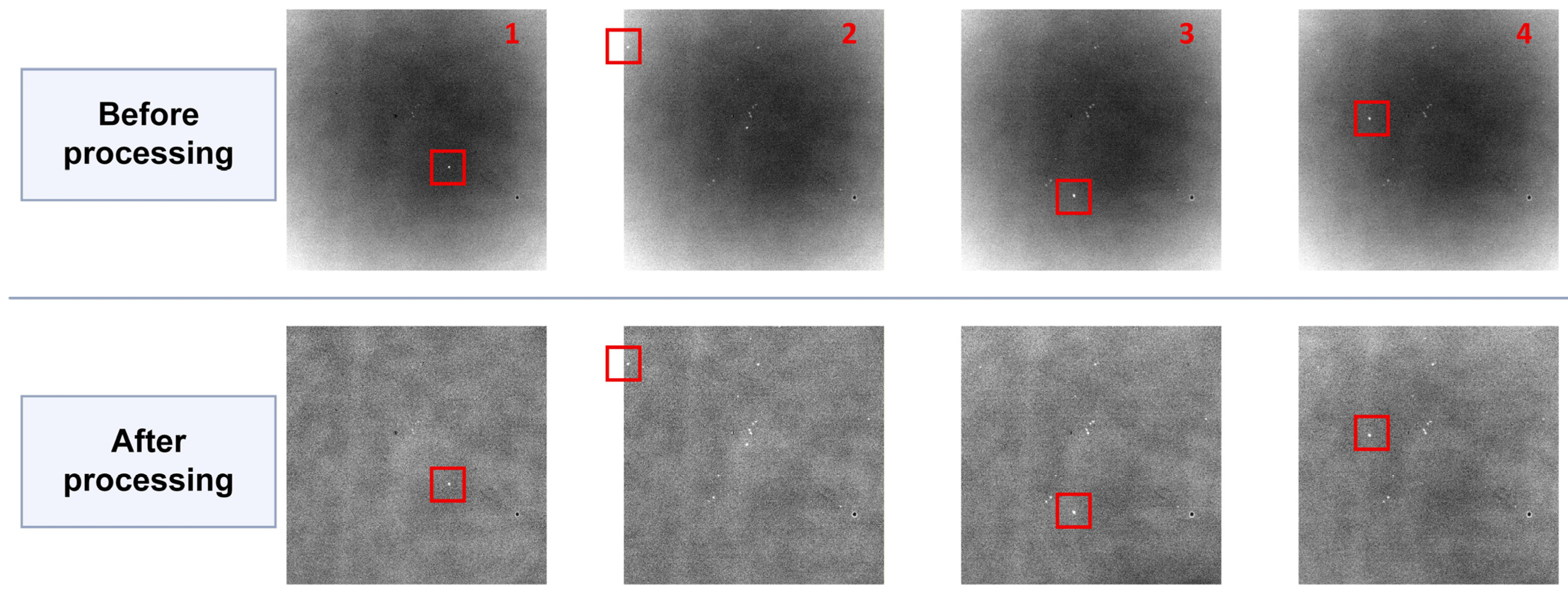
Figure 4, the vignette fields recovered by the three methods and their final correction results are further visualized. The correction performance of each method is analyzed and summarized based on the measured results.
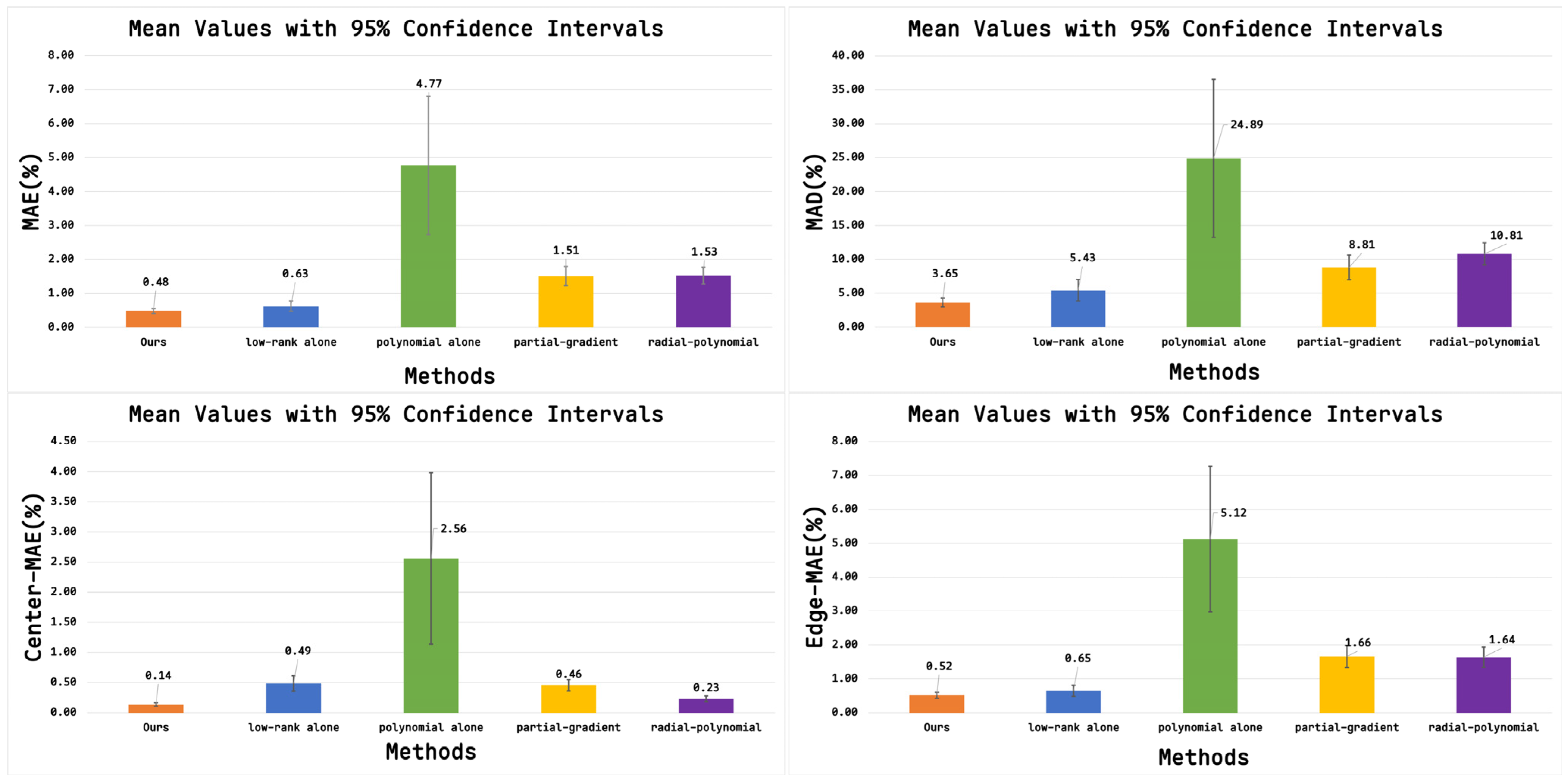
For the four datasets, the results of the three methods in terms of MAE, MAD, Center-MAE, and Edge-MAE are shown in
Figure 5. The proposed full method achieves the best overall performance among the three ablation variants, with MAE, MAD, Center-MAE, and Edge-MAE values of 0.48%, 3.65%, 0.14%, and 0.52%, respectively. Compared with the low-rank-only method, these four metrics are reduced by 23.8%, 32.8%, 71.4%, and 20.0%, respectively. Compared with the polynomial-only method, the reductions are 89.9%, 85.3%, 94.5%, and 89.8%, respectively. These results indicate that low-rank modeling can effectively extract the common vignette structure, while polynomial fitting further improves the smoothness and correction accuracy of vignette estimation.
To provide a more comprehensive comparison, two representative external baseline methods were included in addition to the ablation variants. The first baseline is a non-radial gradient-based method, which represents single-image prior-based correction strategies. This method estimates the low-frequency vignette field from the horizontal and vertical image gradients in the logarithmic domain and uses robust weighting to reduce the influence of strong scene edges. Since it does not impose radial symmetry, it can describe general two-dimensional low-frequency variations, but it remains sensitive to scene-dependent gradients.
The second baseline is a deformable polynomial fitting method, which represents parameterized radial or deformable vignetting models. It first estimates a smooth low-frequency field from a single vignetted image and then fits a deformable radial polynomial model with adjustable center and elliptical deformation. This strategy introduces stronger spatial smoothness and geometric constraints, but it lacks the multi-frame shared-structure constraint used in the proposed method.
All parameter values listed in
Table 3 were fixed for all datasets without dataset-specific tuning. Ground-truth images were used only to calculate the evaluation metrics and were not involved in parameter selection or vignette-field estimation.
As shown in
Table 4, the proposed method achieves consistently lower errors than the two external baseline methods across all four metrics. Specifically, the partial-gradient baseline obtains MAE, MAD, Center-MAE, and Edge-MAE values of 1.51%, 8.81%, 0.46%, and 1.66%, respectively, whereas the proposed method reduces them to 0.48%, 3.65%, 0.14%, and 0.52%. This corresponds to reductions of approximately 68.2%, 58.6%, 69.6%, and 68.7%, respectively. Compared with the radial-polynomial baseline, whose corresponding errors are 1.53%, 10.81%, 0.23%, and 1.64%, the proposed method reduces these four metrics by approximately 68.6%, 66.2%, 39.1%, and 68.3%, respectively.
These results indicate that single-image prior-based methods are less robust when scene-dependent low-frequency variations are mixed with the vignette component. The partial-gradient method is affected by image gradients caused by terrain textures or radiometric transitions, while the radial-polynomial method is constrained by its parametric radial assumption and may not fully describe non-ideal or asymmetric edge attenuation. In contrast, the proposed method first extracts the shared vignette-related component from multiple frames and then refines it through polynomial fitting, leading to better global accuracy and more stable correction in both central and edge regions.
To examine whether the explicit rank-1 model sacrifices performance relative to a general low-rank constraint, a nuclear-norm-based standard RPCA baseline [
29,
30] was additionally implemented. Standard RPCA estimates the low-rank and sparse components by solving
Here, denotes the nuclear norm, defined as the sum of the singular values of , and promotes sparsity in the non-shared component. Unlike the proposed model , standard RPCA does not prescribe the rank of . For fairness, both methods used all available frames and the same logarithmic transformation, polynomial post-fitting, gain construction, and evaluation metrics. Standard RPCA was performed at one-quarter linear spatial resolution and resized to the original resolution using bicubic interpolation.
As shown in
Table 5, standard RPCA obtains slightly lower mean errors than the proposed method, but the absolute differences in MAE, MAD, Center-MAE, and Edge-MAE are only 0.02, 0.19, 0.02, and 0.01 percentage points, respectively. In contrast, the proposed method reduces the cross-dataset standard deviations of MAE, MAD, and Edge-MAE by approximately 29.2%, 14.1%, and 40.0%, respectively, while the Center-MAE standard deviation remains unchanged. These results indicate that the general low-rank model provides a small improvement in mean accuracy, whereas the explicit rank-1 model provides comparable accuracy, lower cross-dataset variability, and a more direct physical representation of the shared vignette field.
3.4. Convergence, Computational Cost, and Parameter Sensitivity
All experiments were implemented in MATLAB R2025a Update 1 and executed on a workstation equipped with an Intel Core i7-13700F CPU (16 cores and 24 logical processors) and 64 GB of RAM. The current implementation uses double-precision computation and does not explicitly employ GPU acceleration.
To evaluate the engineering feasibility of the proposed method, the computational cost was measured over 28 dataset settings using 100 frames of size 2048 × 2048 for vignette-field estimation.
For a 100-frame stack, a single double-precision matrix of size
requires approximately 3.13 GB. As shown in
Table 7, because the current MATLAB implementation simultaneously maintains several matrices of this size, the core matrix storage is approximately 21.9 GB, and the peak memory requirement is estimated to be 22–30 GB when temporary arrays are included. This substantial memory requirement limits the current implementation primarily to offline ground-based processing on workstations rather than resource-constrained onboard or real-time deployment. It should be noted that this estimate reflects the present implementation rather than an irreducible theoretical cost of the proposed model. Future work will therefore investigate block-wise processing, frame batching, reduced-precision storage, and incremental low-rank updates to reduce memory consumption and improve deployment efficiency.
To further evaluate the practical applicability of the proposed method, this section analyzes the convergence behavior, computational cost, and sensitivity to the polynomial order. These factors are important for applying the method to high-resolution multi-frame images, especially for 2048 × 2048 remote sensing data.
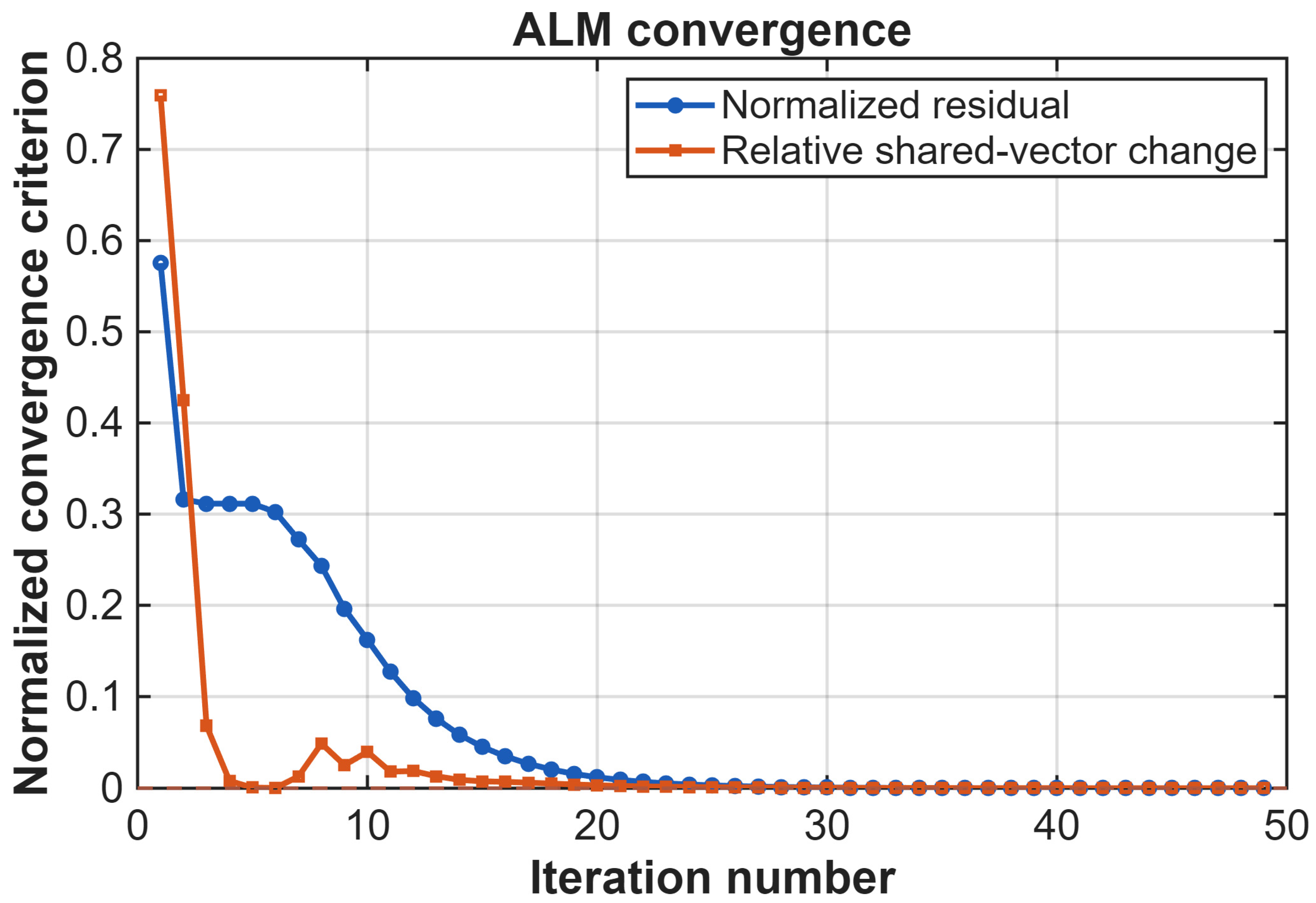
In the ALM-based low-rank decomposition, convergence is monitored using two criteria: the normalized reconstruction residual and the relative change of the shared vignette vector. The normalized residual measures whether the constraint is gradually satisfied, while the relative vector change reflects whether the estimated shared vignette field becomes stable. The iteration is terminated when both criteria are smaller than the predefined thresholds, or when the maximum number of iterations is reached. In this study, the residual threshold, vector-change threshold, and maximum number of iterations were set to , and 200, respectively.
Figure 7 presents the convergence history for DATA-3, where both stopping criteria were satisfied after 49 iterations. As shown in
Table 8, across the 28 test sequences derived from the four base datasets, the algorithm required 49.21 ± 0.42 iterations (mean ± SD), with a range of 49–50 iterations. All runs converged before reaching the maximum limit of 200 iterations, indicating consistent convergence behavior across the evaluated datasets. This indicates that the ALM-based decomposition reaches a stable numerical solution for the tested 2048 × 2048 multi-frame image stack.
Let denote the number of pixels in each image, the number of input frames, the number of ALM iterations, and the number of polynomial basis terms. The logarithmic transformation and vectorization require operations. In the ALM stage, each iteration updates the shared component, sparse component, residual, and Lagrange multiplier over the data matrix , resulting in a per-iteration cost of . Therefore, the ALM decomposition has a total complexity of . The polynomial fitting stage requires , and the final pixel-wise correction requires . Overall, the computational complexity is approximately , with a memory complexity of . Since in this study, , and the polynomial fitting cost is much smaller than the ALM decomposition cost for 2048 × 2048 multi-frame images.
The number of input frames determines the amount of redundant information available for separating the shared vignette field from scene-dependent variations. Insufficient frames may result in an unstable estimate because the diversity of scene content is inadequate to suppress non-shared structures. To evaluate this effect, the number of frames used for vignette estimation was set to , and the results were compared with those obtained using all available frames.
As shown in
Table 9, the results show that using only five frames leads to substantial performance degradation, indicating that insufficient scene diversity cannot reliably separate the shared vignette field from non-shared image content. Although the errors generally decrease as more frames are included, the trend is not strictly monotonic; the results at
are slightly worse than those at
. This suggests that performance depends not only on the number of frames but also on the scene composition of the selected subset. When
increases to 100, all four metrics are within approximately 10% of the all-frame results. Therefore, approximately 100 frames can be regarded as the empirical minimum for stable recovery under the tested conditions, rather than a universal theoretical threshold.
The polynomial order is an important hyperparameter because it controls the balance between model flexibility and spatial smoothness. A low polynomial order may underfit complex vignette distributions, whereas an excessively high order may introduce unnecessary local fluctuations and reduce the physical smoothness of the estimated field. Therefore, a sensitivity analysis was conducted by comparing different polynomial orders under the same datasets and evaluation metrics. The results show that provides a good trade-off between correction accuracy and stability, and it was therefore used in all experiments.
As shown in
Table 10, the polynomial order increases from
to
, the correction errors decrease markedly, with MAE, MAD, and Edge-MAE reduced from 1.37%, 13.48%, and 1.80% to 0.42%, 3.72%, and 0.50%, respectively. This demonstrates that very low-order polynomials tend to underfit the vignette field. Further increasing the order to
or
does not provide consistent improvement: the MAD is slightly reduced at
, but the MAE and Center-MAE increase, suggesting potential local instability or overfitting. The runtime varies only slightly across different orders, indicating that the overall computational cost is dominated by the low-rank decomposition rather than the polynomial fitting. Therefore,
was adopted as a balanced setting between fitting accuracy, spatial stability, and computational cost.
The regularization parameter
controls the balance between the shared low-rank component and the sparse non-shared component. An inappropriate value may cause the shared vignette structure to leak into the sparse component or allow scene-dependent variations to remain in the estimated low-rank component. Therefore, the sensitivity to
was evaluated on the representative DATA-0-3 dataset using all available frames. Specifically,
was defined as
, where
and the scaling factor was set to
. All other parameters were kept unchanged. The results are presented in
Table 5.
As shown in
Table 11, as the scaling factor
varied from 0.25 to 4, MAE and Edge-MAE remained unchanged at 0.22% and 0.24%, respectively. MAD varied only between 2.25% and 2.31%, while Center-MAE varied between 0.07% and 0.08%. These results indicate that the proposed method is insensitive to
within the tested range. The default setting
was selected because it achieved the lowest MAD and Center-MAE.
In the present implementation, the low-rank component is explicitly modeled as a rank-1 shared vignette field, , where represents the common spatial vignette vector shared by all frames. Therefore, the rank used in the matrix decomposition is fixed to one in all main experiments. This choice is based on the short-term stability assumption of vignetting, under which multiple images acquired under similar imaging conditions are expected to share the same dominant vignette field.
Since the proposed method explicitly adopts a rank-1 shared vignette model, an additional rank-sensitivity experiment was conducted to examine the effect of rank selection. In this diagnostic experiment, the low-rank component was estimated with different fixed ranks, while the subsequent polynomial fitting and correction procedures were kept unchanged. As shown in
Table 9, increasing the rank changes the balance between average correction accuracy and local error control. A higher rank may improve the representation flexibility of the low-rank component, but it may also absorb scene-dependent structures or local fluctuations, leading to increased worst-case errors. This result supports the use of the rank-1 shared model under the short-term stability assumption and also indicates that adaptive-rank modeling may be necessary for more complex cases.
To evaluate the influence of rank selection, a diagnostic rank-sensitivity experiment was conducted while keeping the subsequent polynomial fitting and correction procedures unchanged. As shown in
Table 12, the rank-1 setting achieves the lowest errors, with MAE, MAD, Center-MAE, and Edge-MAE values of 0.20%, 1.14%, 0.07%, and 0.15%, respectively. When the rank is increased to 5, these errors increase to 0.29%, 1.57%, 0.10%, and 0.30%, respectively. Compared with rank 5, the rank-1 setting reduces MAE, MAD, Center-MAE, and Edge-MAE by approximately 31%, 27%, 30%, and 50%.
This result indicates that the dominant vignette component in the tested data is better represented by a rank-1 shared structure. Increasing the rank does not necessarily improve correction accuracy; instead, it may absorb scene-dependent variations or local residual structures into the low-rank component, reducing the physical stability of the estimated vignette field. Therefore, the rank-1 setting used in the proposed method is appropriate under the short-term stable vignetting assumption.
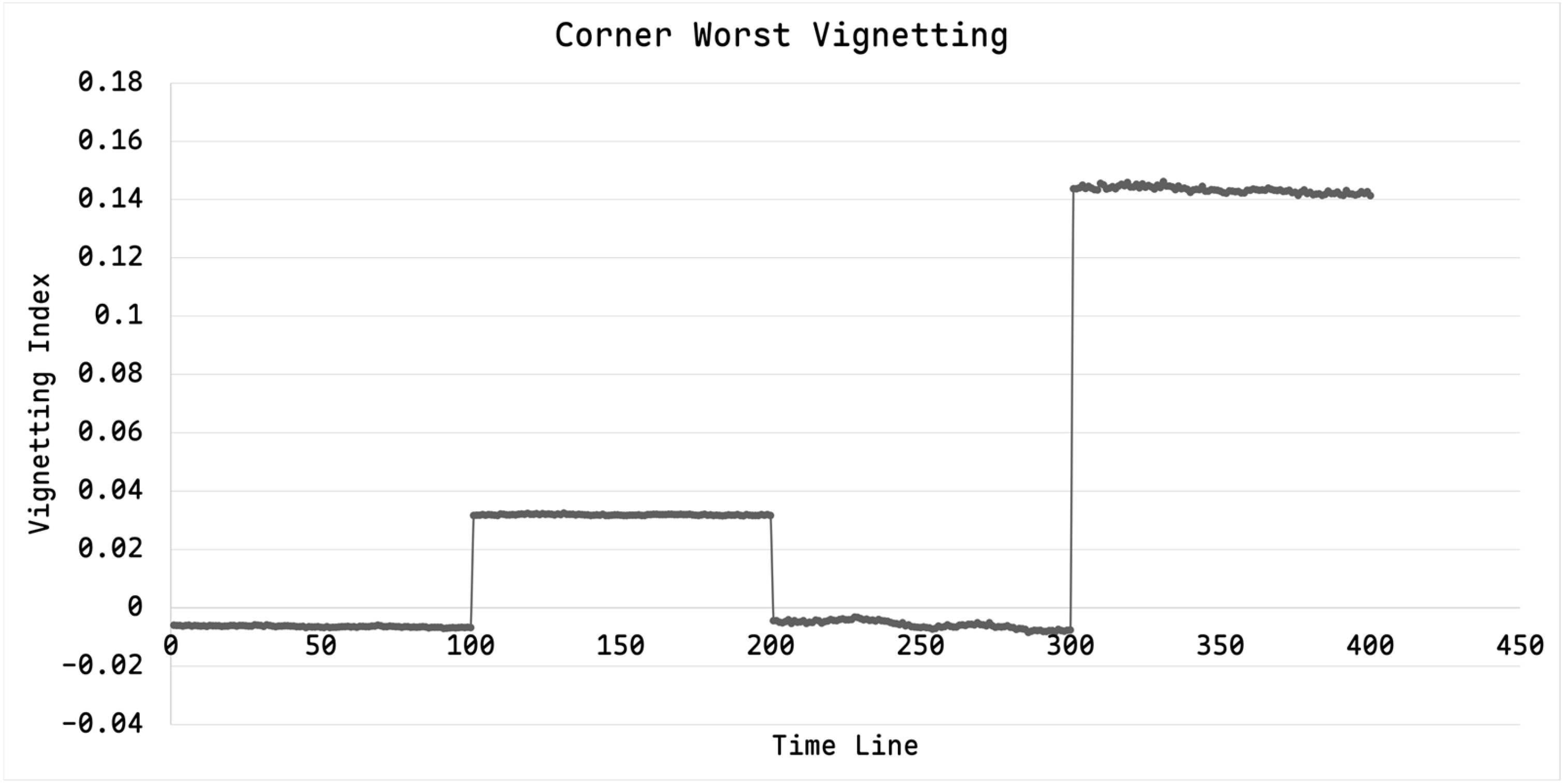
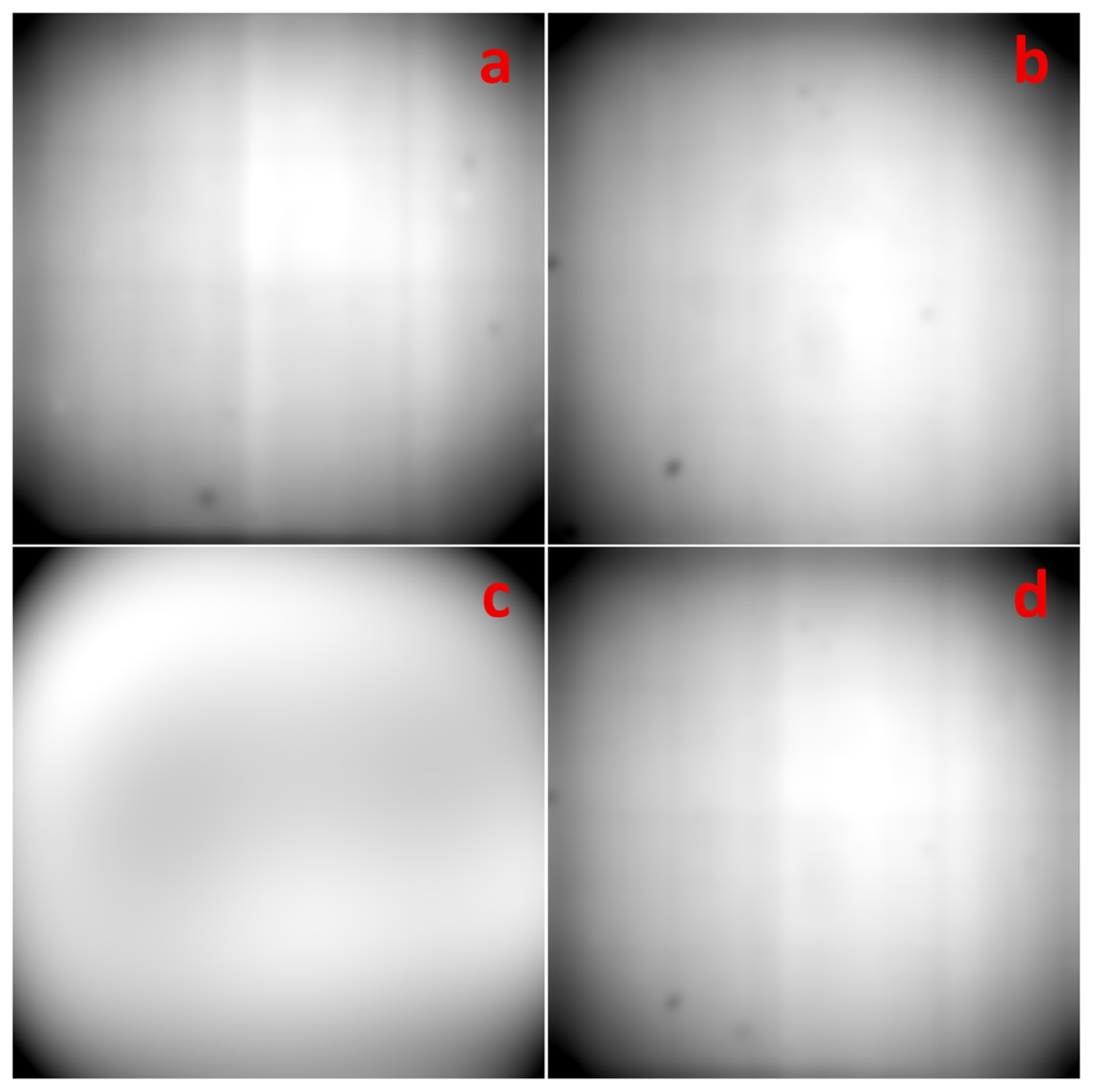
The theoretical field
represents the idealized compromise solution of a single rank-1 shared model. It is not the theoretical output of standard RPCA, which permits multiple low-rank variation modes, as shown in
Figure 8.
As shown in
Table 13, applying a single jointly estimated rank-1 vignette field to the mixed sequence results in MAE values of 0.68% and 0.40% for Data A and Data B, respectively. This asymmetric residual error indicates that the jointly estimated field cannot accurately represent both vignette patterns and instead behaves as a compromise between them. After dividing the sequence into two stable windows and independently estimating the vignette field for each group, the MAE values decrease to 0.32% and 0.22%, corresponding to reductions of 52.9% and 45.0%, respectively. These results confirm that violation of the shared-field assumption leads to appreciable residual correction errors, whereas separate-window estimation effectively restores the validity of the rank-1 model and substantially improves correction accuracy.
Standard RPCA was additionally examined as a general low-rank reference. Because it does not enforce , it can preserve multiple low-rank variation modes when the sequence contains different vignette fields. However, standard RPCA does not automatically provide one vignette field for each temporal segment. If its low-rank columns are aggregated into a single field, the resulting estimate still cannot accurately represent both and . Temporal windowing or clustering of the low-rank columns is therefore still required.
In practical applications, the vignetting index introduced above can provide a measurable basis for detecting changes in the vignette field. For a sequential image stack, the index can be calculated for each frame or short sliding window and smoothed to suppress random fluctuations. A candidate transition can then be detected by comparing the median vignetting indices of two adjacent windows. Specifically, a change point is declared when their difference exceeds a threshold determined from the index fluctuations observed under stable imaging conditions and persists for several consecutive frames. A minimum segment length can also be imposed to avoid excessive segmentation. After detection, the sequence is divided into separate stability windows, and the proposed rank-1 estimation is performed independently within each window. Nevertheless, automatic threshold selection may still be affected by scene-content changes and measurement noise. Therefore, developing and validating an adaptive change-point detector based on the vignetting index will be considered in future work.