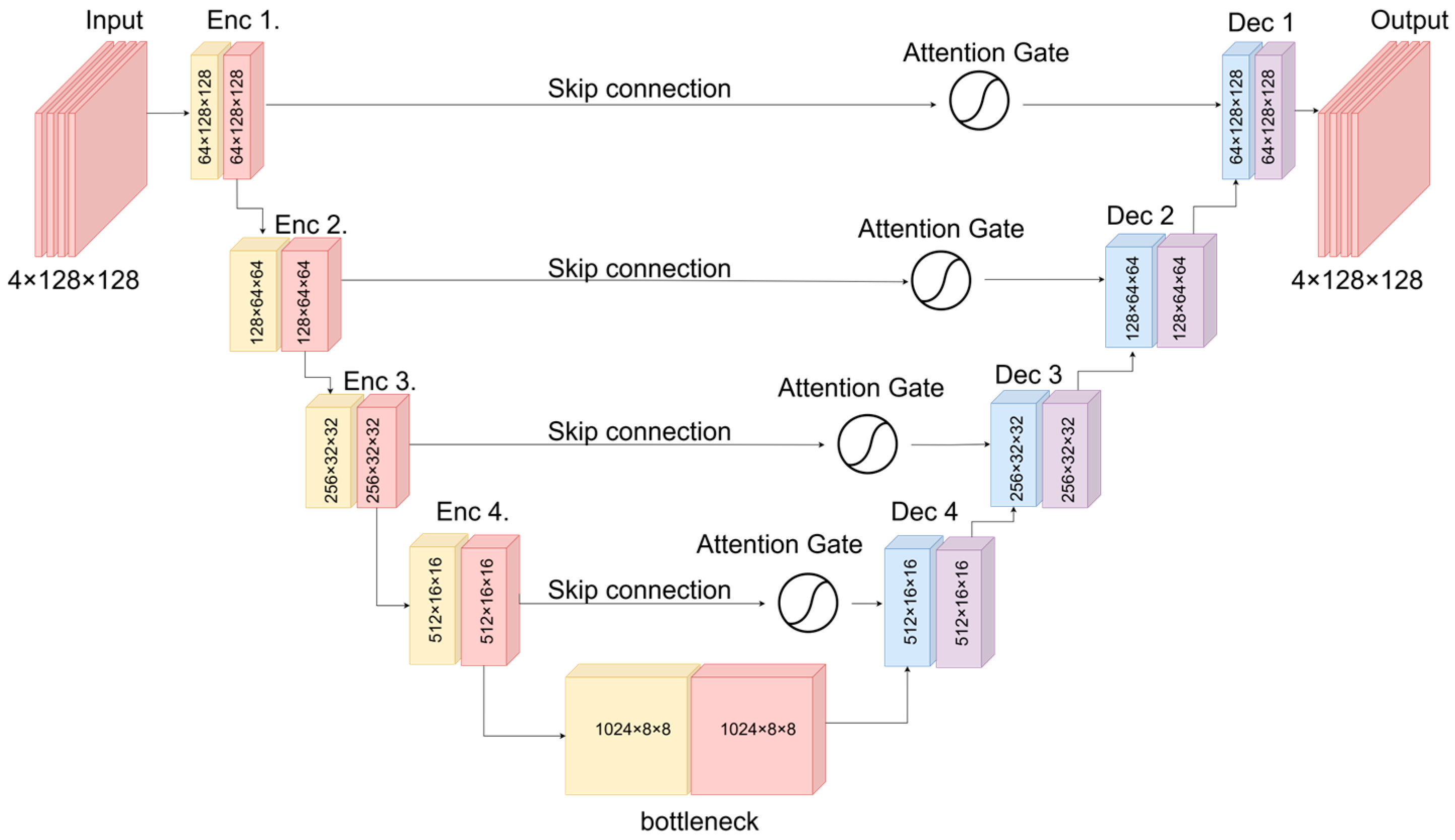
Figure 1.
WaveletBasedAttention-Net architecture (DWT→4-band U-Net→IDWT) with hop connections and 1024 filter bottleneck.
Figure 1.
WaveletBasedAttention-Net architecture (DWT→4-band U-Net→IDWT) with hop connections and 1024 filter bottleneck.
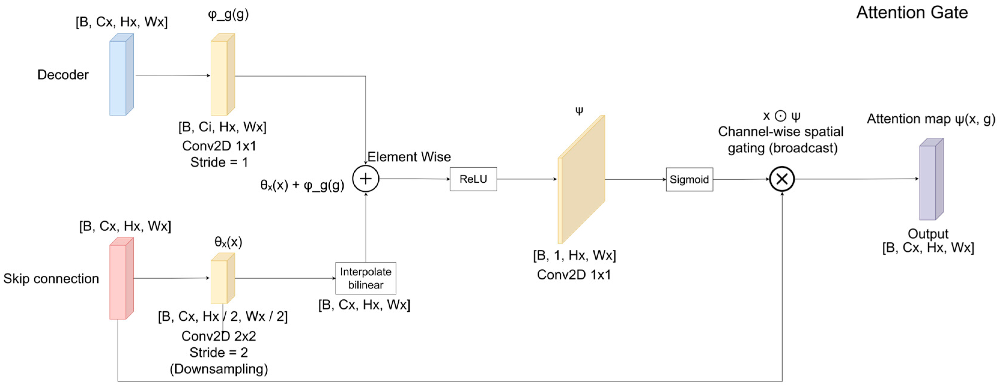
Figure 2.
Attention gate (AG) mechanism integrated into the skip connections of the proposed Attention U-Net architecture.
Figure 2.
Attention gate (AG) mechanism integrated into the skip connections of the proposed Attention U-Net architecture.
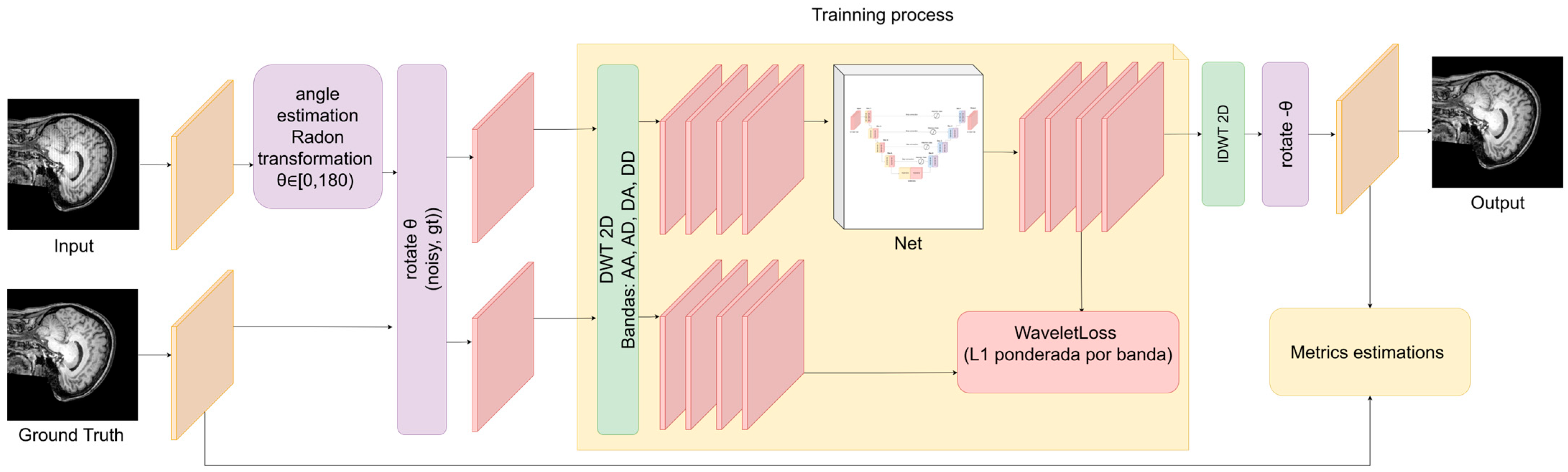
Figure 3.
Training and evaluation pipeline: Radon-guided rotation, DWT decomposition, wavelet-based network processing, IDWT reconstruction, and inverse rotation. Loss is computed per band, and metrics are evaluated on the reconstructed image.
Figure 3.
Training and evaluation pipeline: Radon-guided rotation, DWT decomposition, wavelet-based network processing, IDWT reconstruction, and inverse rotation. Loss is computed per band, and metrics are evaluated on the reconstructed image.
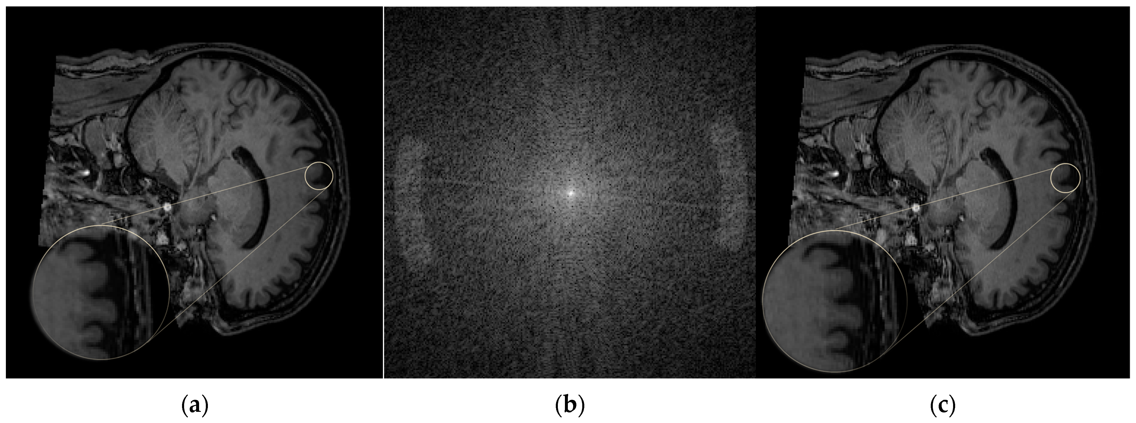
Figure 4.
Ringing artifact: image appearance and k-space signature. (a) Artifact-free brain MRI. (b) k-space signature showing the magnitude spectrum of the artifact component, computed as log (1 + . (c) Image with the ringing artifact; ellipses show edge-aligned oscillations adjacent to a high-contrast boundary.
Figure 4.
Ringing artifact: image appearance and k-space signature. (a) Artifact-free brain MRI. (b) k-space signature showing the magnitude spectrum of the artifact component, computed as log (1 + . (c) Image with the ringing artifact; ellipses show edge-aligned oscillations adjacent to a high-contrast boundary.
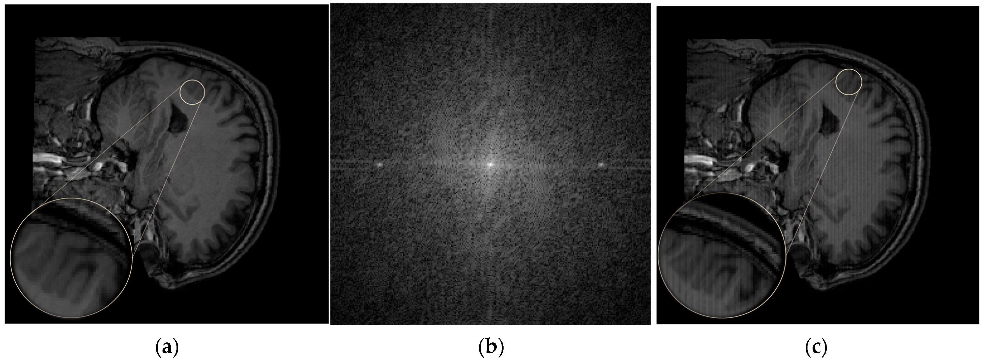
Figure 5.
Herringbone artifact: image appearance and k-space signature. (a) Artifact-free brain MRI. (b) k-space signature showing the log-magnitude spectrum of the artifact component computed as log (1 + (c) Image with herringbone artifact; the ellipse shows the banding pattern in gray matter.
Figure 5.
Herringbone artifact: image appearance and k-space signature. (a) Artifact-free brain MRI. (b) k-space signature showing the log-magnitude spectrum of the artifact component computed as log (1 + (c) Image with herringbone artifact; the ellipse shows the banding pattern in gray matter.
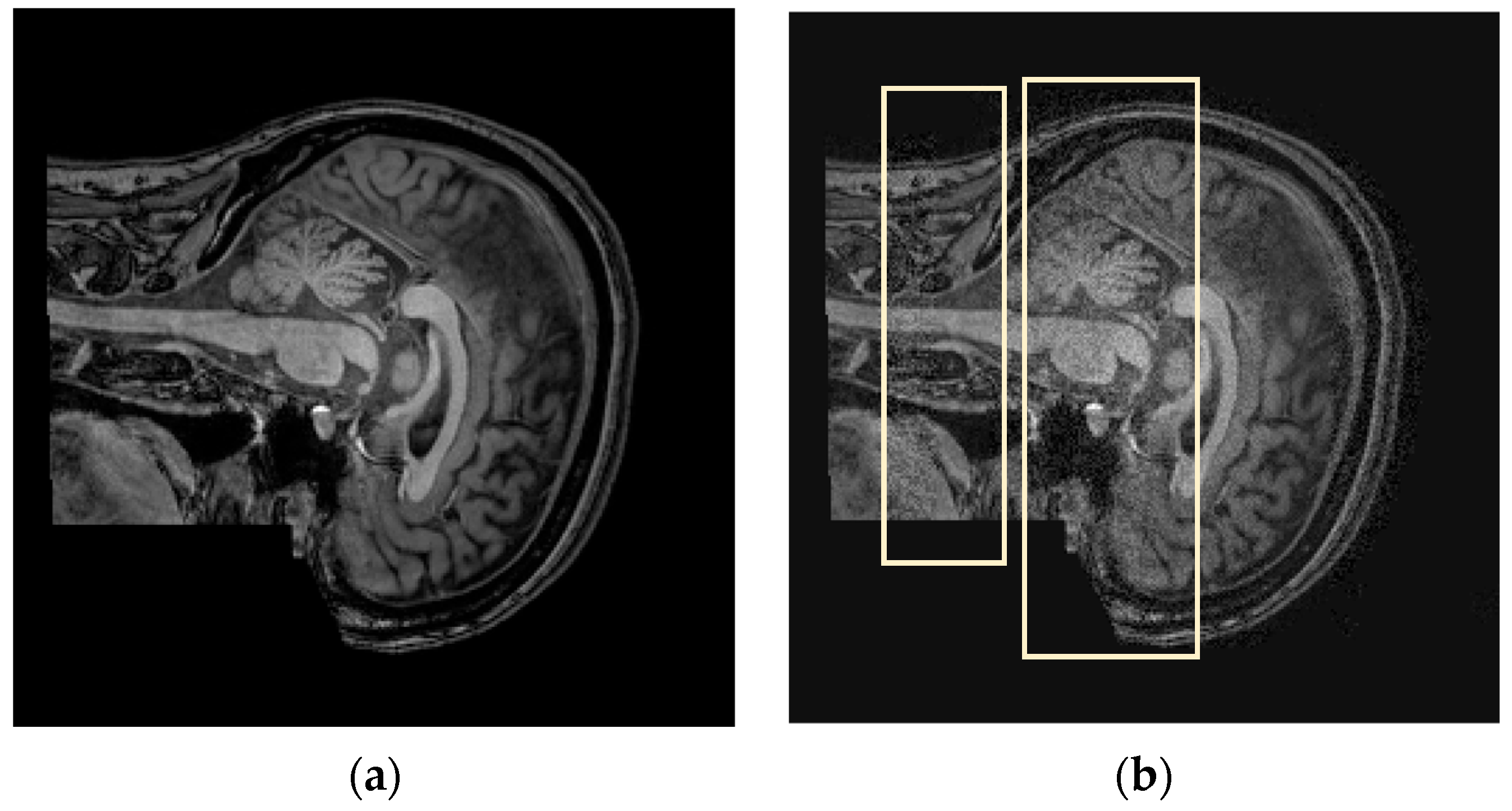
Figure 6.
Zipper artifact: image appearance. (a) Artifact-free brain MRI. (b) Image with the zipper artifact; rectangles show the vertical noise patterns.
Figure 6.
Zipper artifact: image appearance. (a) Artifact-free brain MRI. (b) Image with the zipper artifact; rectangles show the vertical noise patterns.
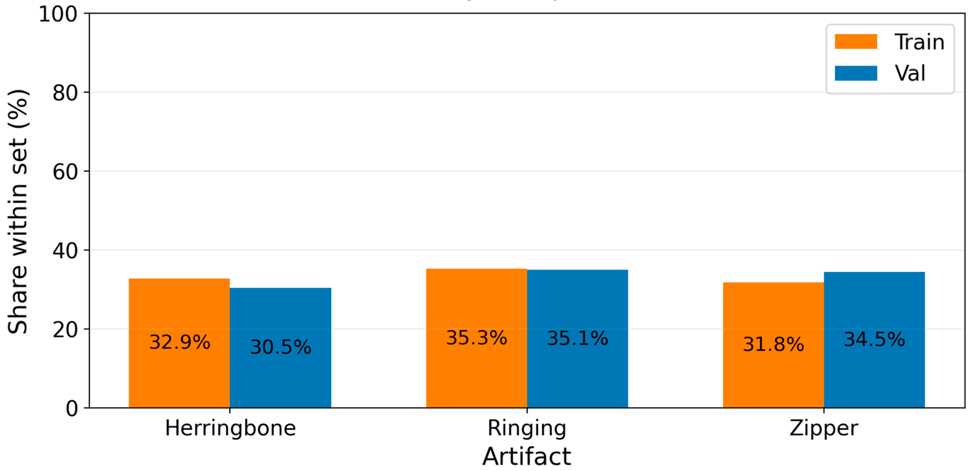
Figure 7.
Percentage distribution of artifact types (ringing, herringbone, and zipper) across the training and validation partitions.
Figure 7.
Percentage distribution of artifact types (ringing, herringbone, and zipper) across the training and validation partitions.
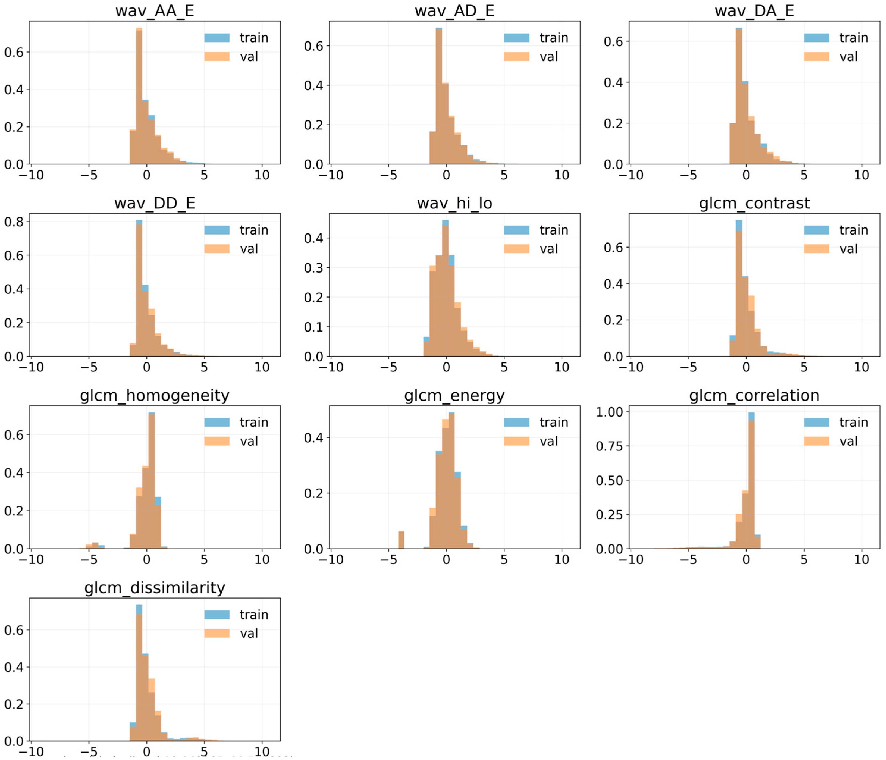
Figure 8.
Distribution of wavelet and GLCM descriptors in the training and validation partitions.
Figure 8.
Distribution of wavelet and GLCM descriptors in the training and validation partitions.
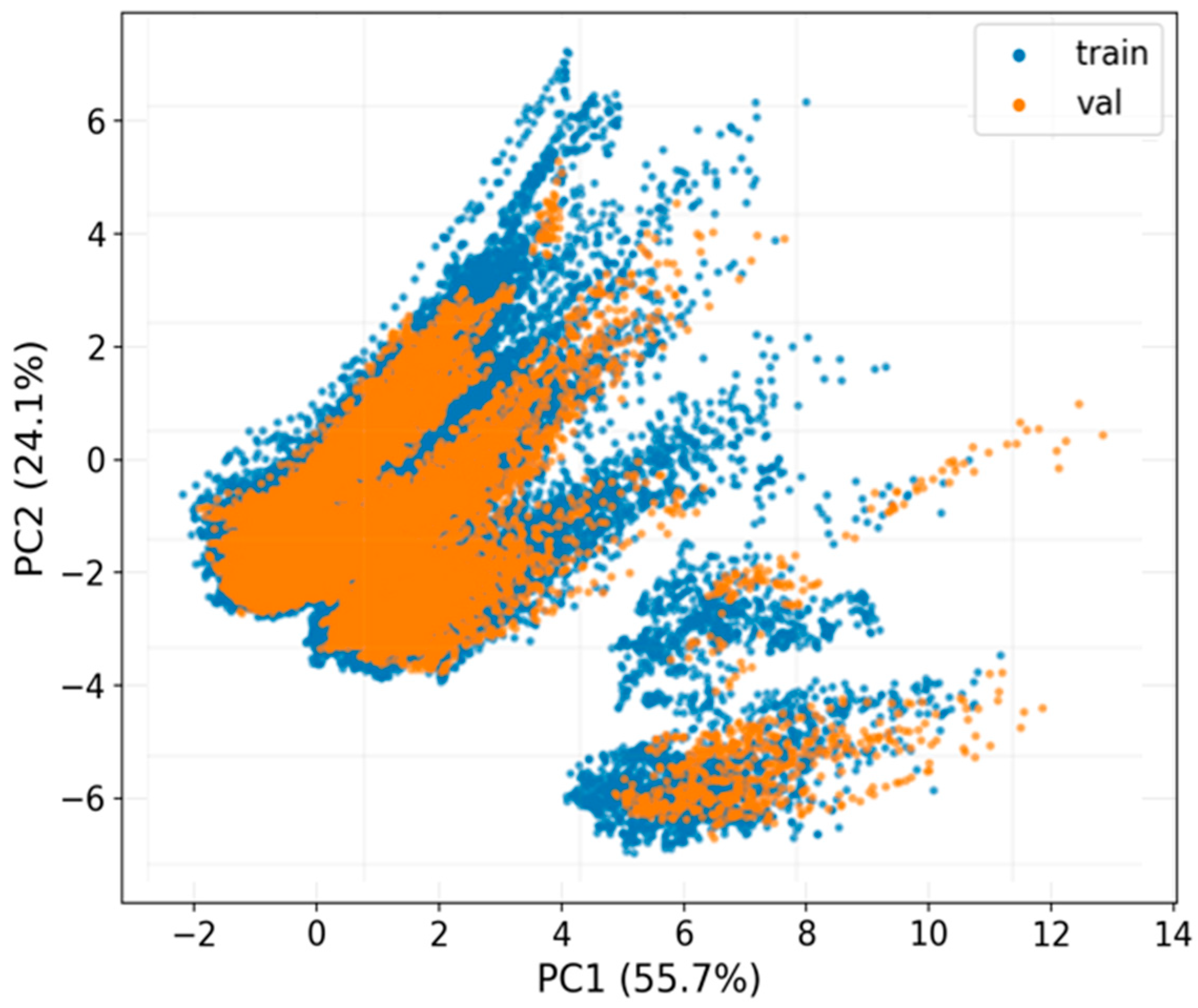
Figure 9.
PCA projection of wavelet + GLCM features: training vs. validation distribution comparison.
Figure 9.
PCA projection of wavelet + GLCM features: training vs. validation distribution comparison.
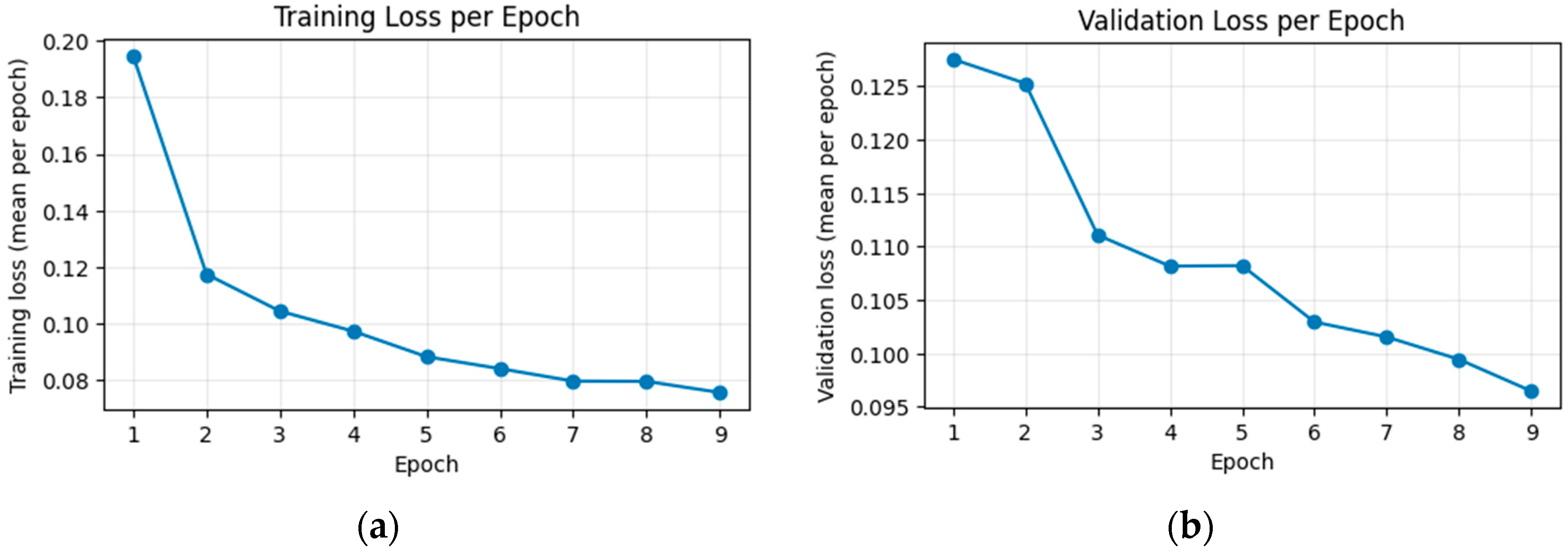
Figure 10.
Evolution of the compound loss across epochs for the training and validation partitions. (a) Training loss; (b) validation loss.
Figure 10.
Evolution of the compound loss across epochs for the training and validation partitions. (a) Training loss; (b) validation loss.
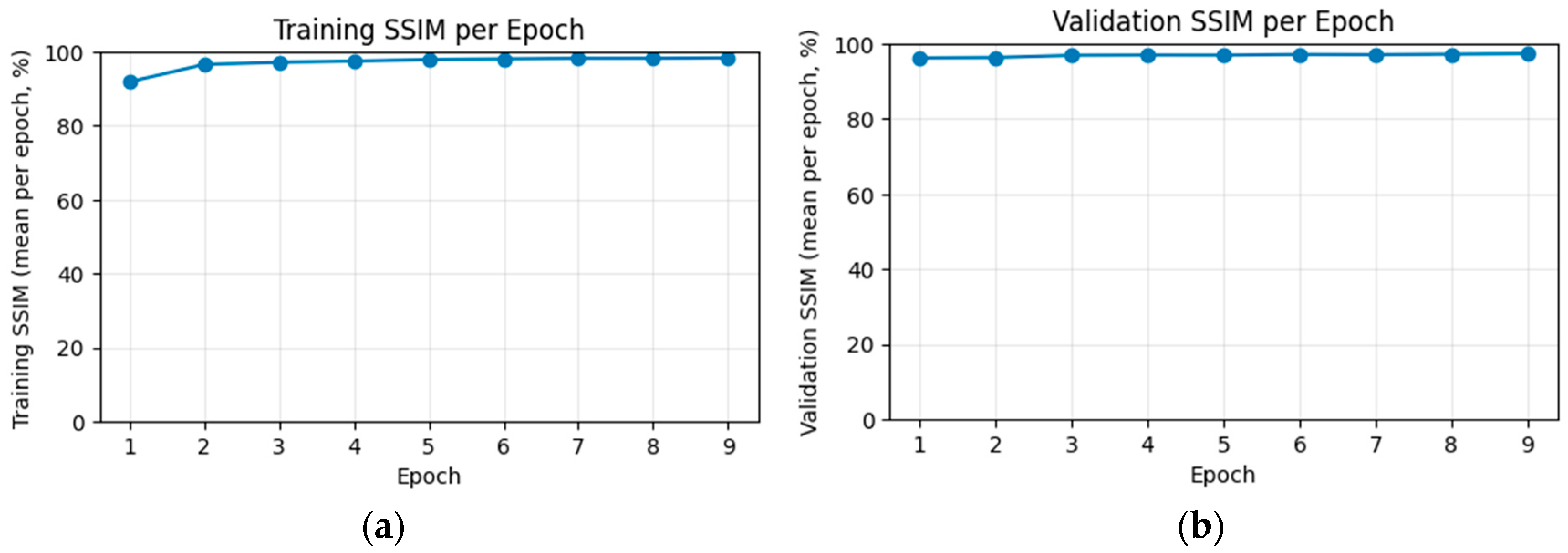
Figure 11.
Evolution of the SSIM metric across epochs for the training and validation partitions. (a) Training SSIM; (b) validation SSIM.
Figure 11.
Evolution of the SSIM metric across epochs for the training and validation partitions. (a) Training SSIM; (b) validation SSIM.
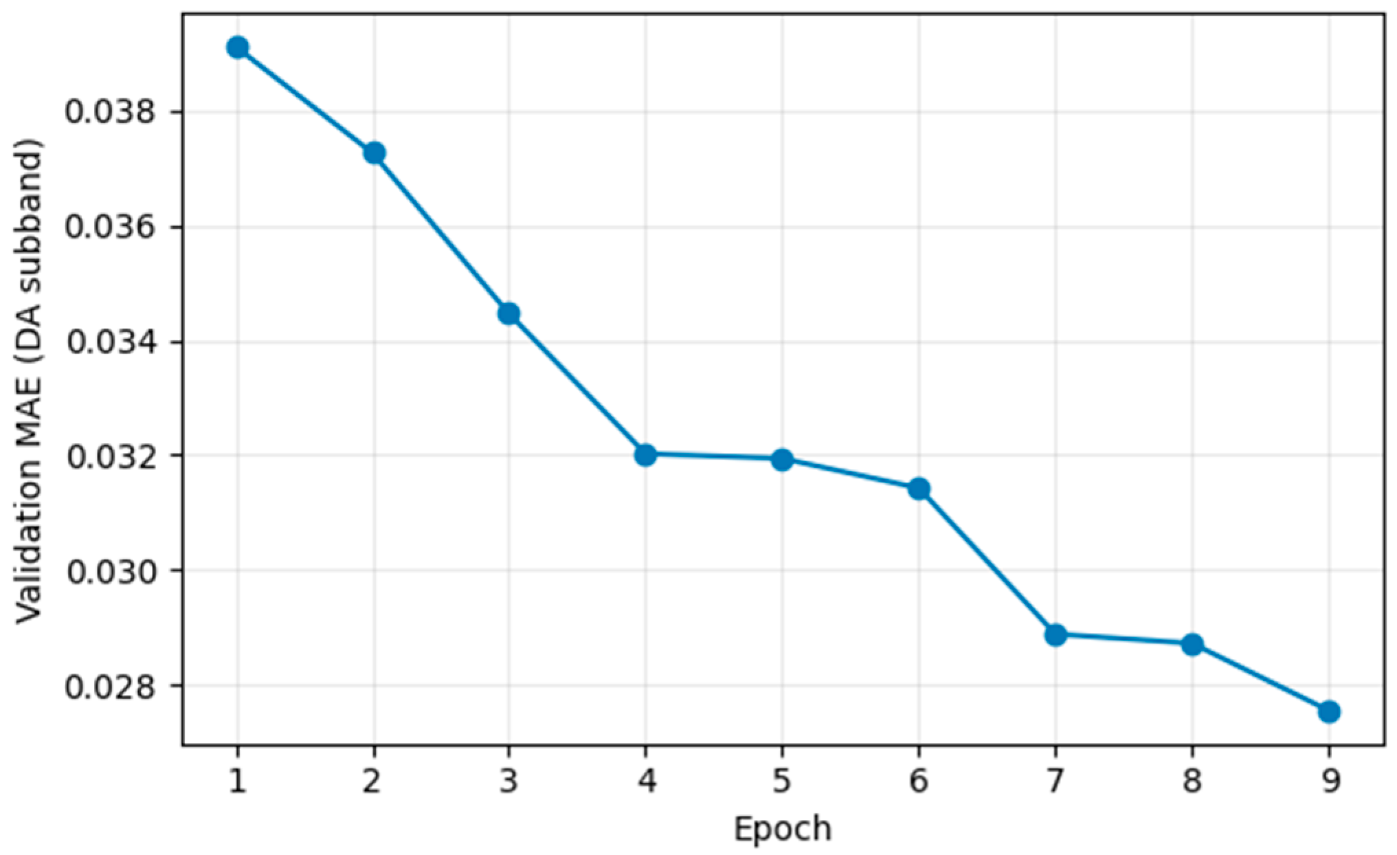
Figure 12.
Evolution of the validation MAE across epochs, computed on the high-frequency DA wavelet sub-band.
Figure 12.
Evolution of the validation MAE across epochs, computed on the high-frequency DA wavelet sub-band.
Figure 13.
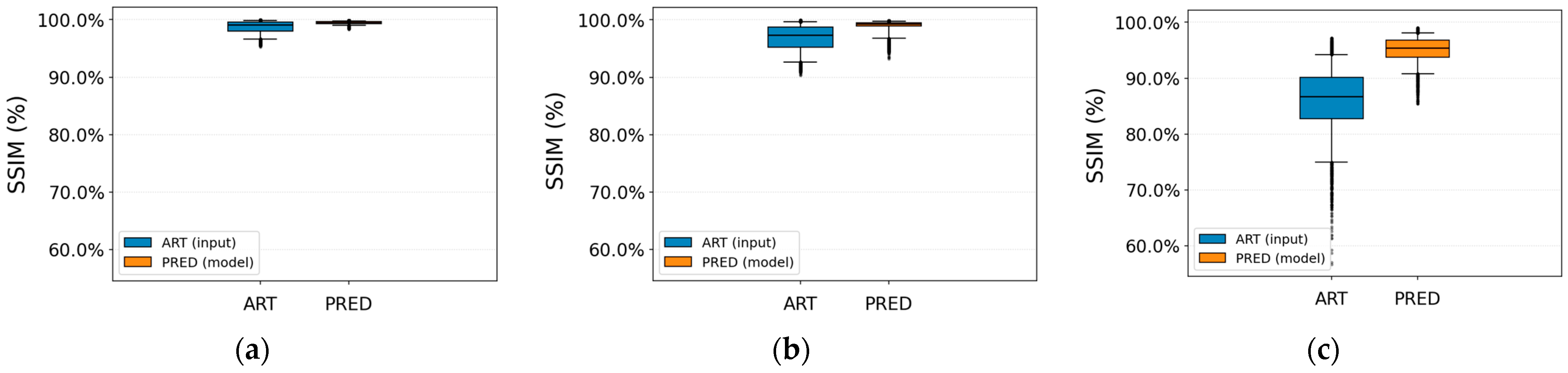
SSIM results by artifact type before and after correction. (a) Ringing artifact; (b) herringbone artifact; (c) zipper artifact.
Figure 13.
SSIM results by artifact type before and after correction. (a) Ringing artifact; (b) herringbone artifact; (c) zipper artifact.
Figure 14.
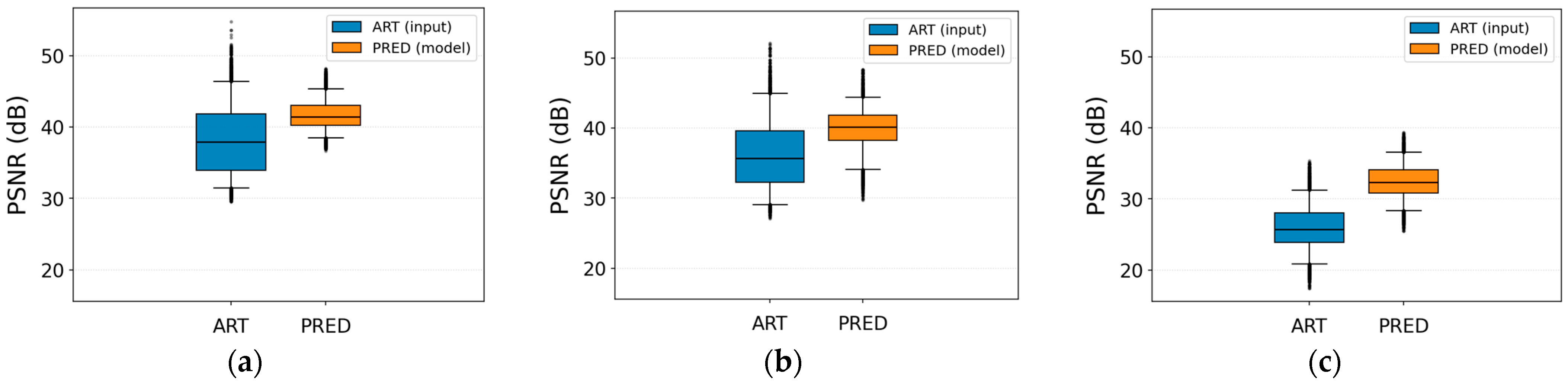
PSNR before and after correction for each artifact type. (a) Ringing artifact; (b) herringbone artifact; (c) zipper artifact.
Figure 14.
PSNR before and after correction for each artifact type. (a) Ringing artifact; (b) herringbone artifact; (c) zipper artifact.
Figure 15.
MSE by wavelet band before and after correction for each artifact type. (a) Ringing artifact; (b) herringbone artifact; (c) zipper artifact.
Figure 15.
MSE by wavelet band before and after correction for each artifact type. (a) Ringing artifact; (b) herringbone artifact; (c) zipper artifact.
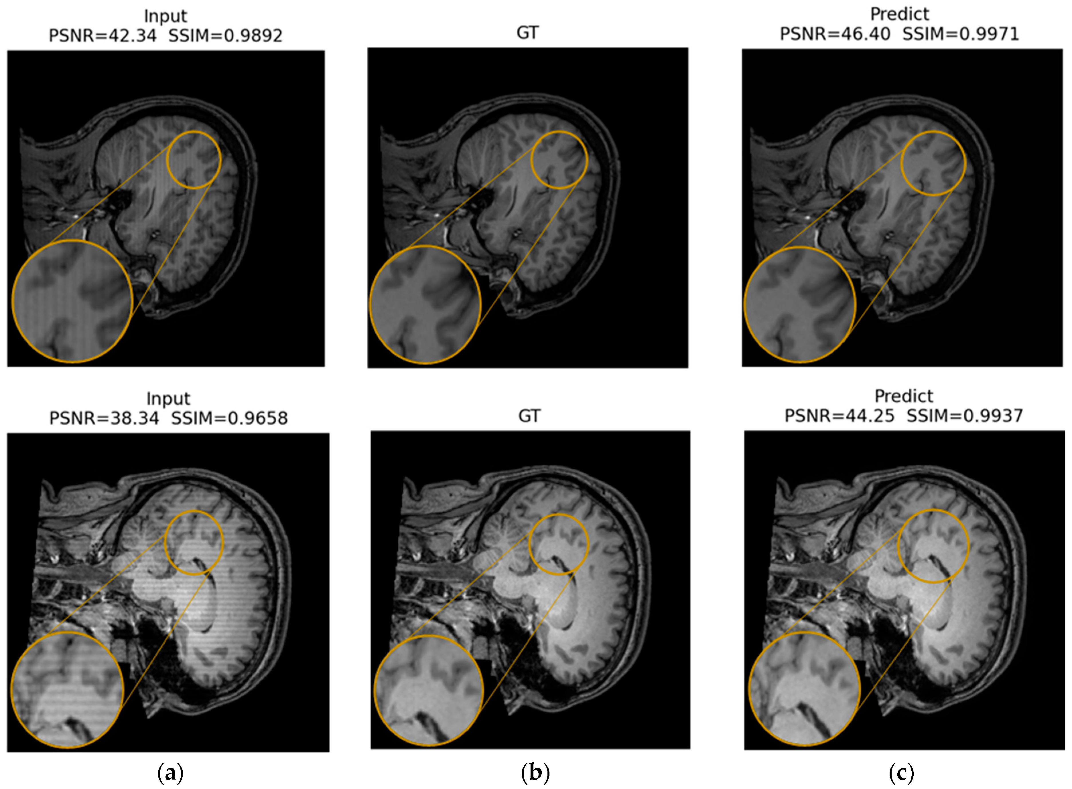
Figure 16.
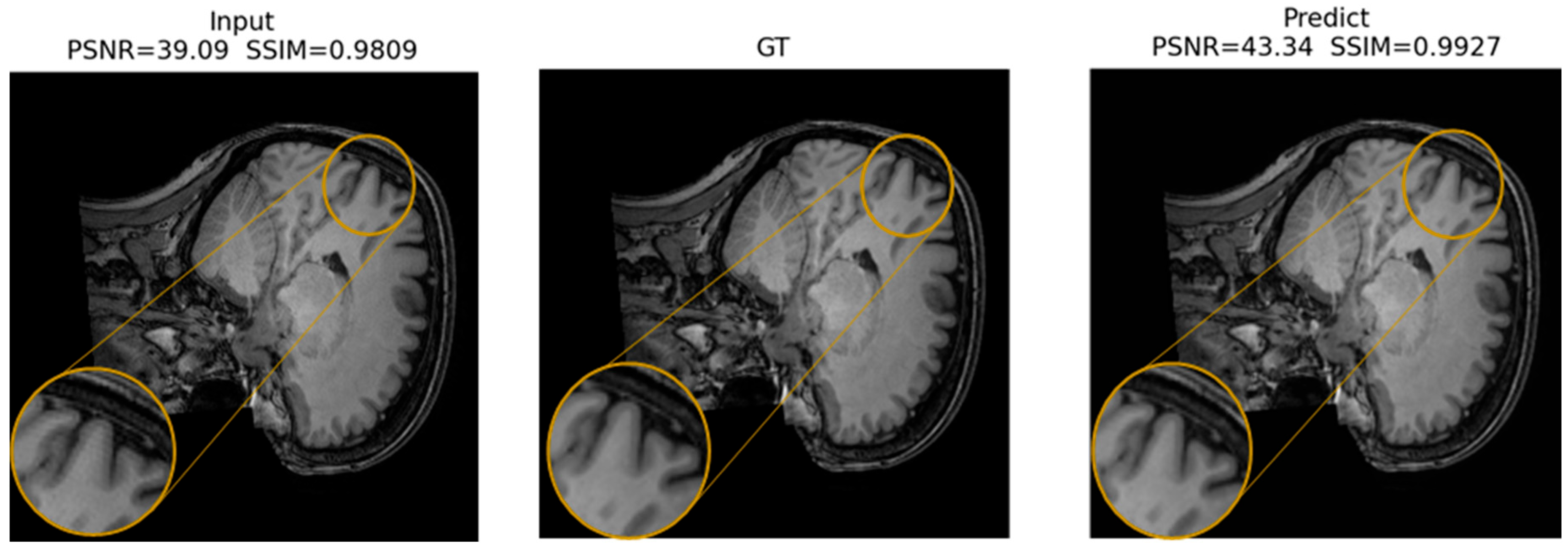
Visual comparison of ringing artifact correction. (a) Artifacted input image (b), ground truth (GT), and (c) model prediction. Highlighted regions show areas affected by the ringing artifact, where the proposed model achieves improved restoration quality, reflected in higher PSNR and SSIM values.
Figure 16.
Visual comparison of ringing artifact correction. (a) Artifacted input image (b), ground truth (GT), and (c) model prediction. Highlighted regions show areas affected by the ringing artifact, where the proposed model achieves improved restoration quality, reflected in higher PSNR and SSIM values.
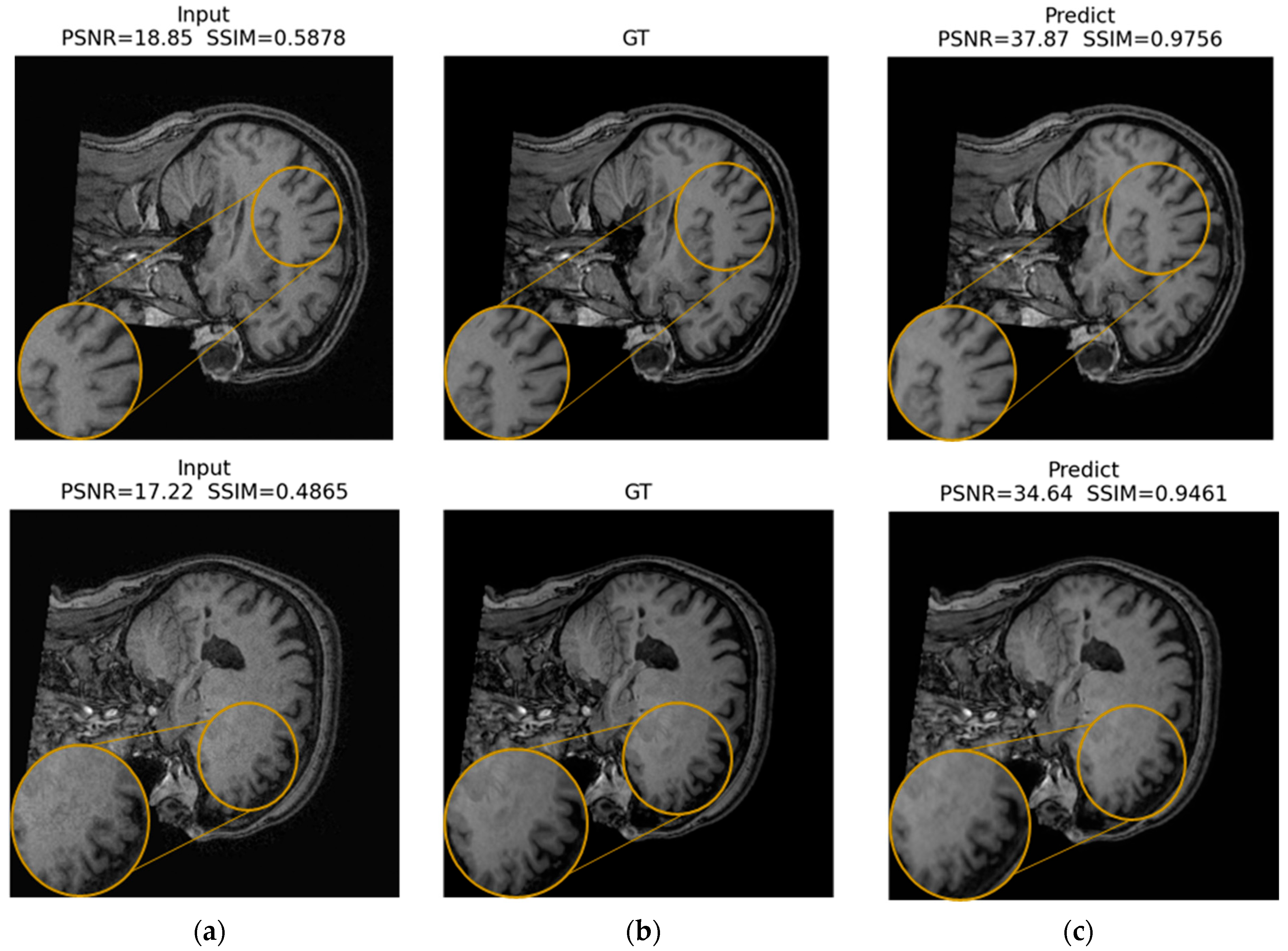
Figure 17.
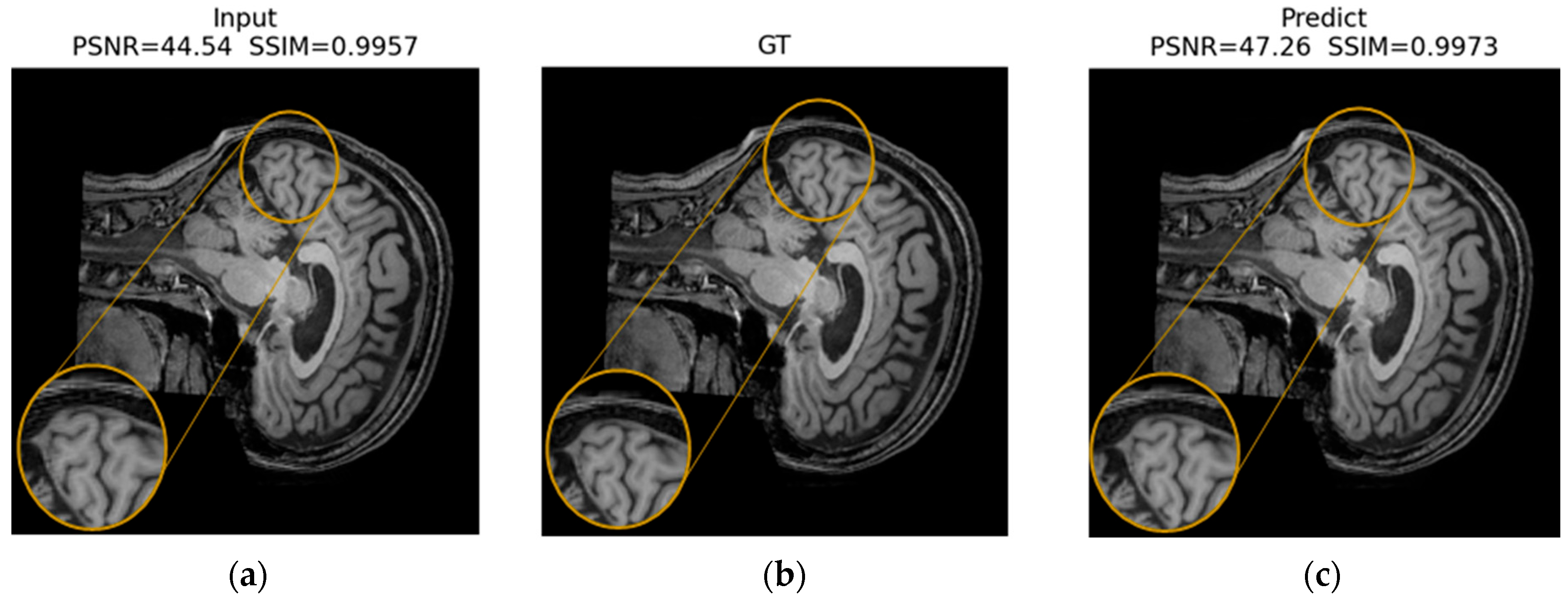
Visual comparison of herringbone artifact correction. (a) Artifacted input image; (b) ground truth (GT); and (c) model prediction. Highlighted regions indicate areas affected by the herringbone artifact, where the proposed model achieves noticeable improvements in image quality, reflected in higher PSNR and SSIM values.
Figure 17.
Visual comparison of herringbone artifact correction. (a) Artifacted input image; (b) ground truth (GT); and (c) model prediction. Highlighted regions indicate areas affected by the herringbone artifact, where the proposed model achieves noticeable improvements in image quality, reflected in higher PSNR and SSIM values.
Figure 18.
Visual comparison of zipper artifact correction. (a) Artifacted input image; (b) ground truth (GT); and (c) model prediction. Highlighted regions indicate areas affected by the zipper artifact, where the proposed model achieves noticeable improvements in image quality, reflected in higher PSNR and SSIM values.
Figure 18.
Visual comparison of zipper artifact correction. (a) Artifacted input image; (b) ground truth (GT); and (c) model prediction. Highlighted regions indicate areas affected by the zipper artifact, where the proposed model achieves noticeable improvements in image quality, reflected in higher PSNR and SSIM values.
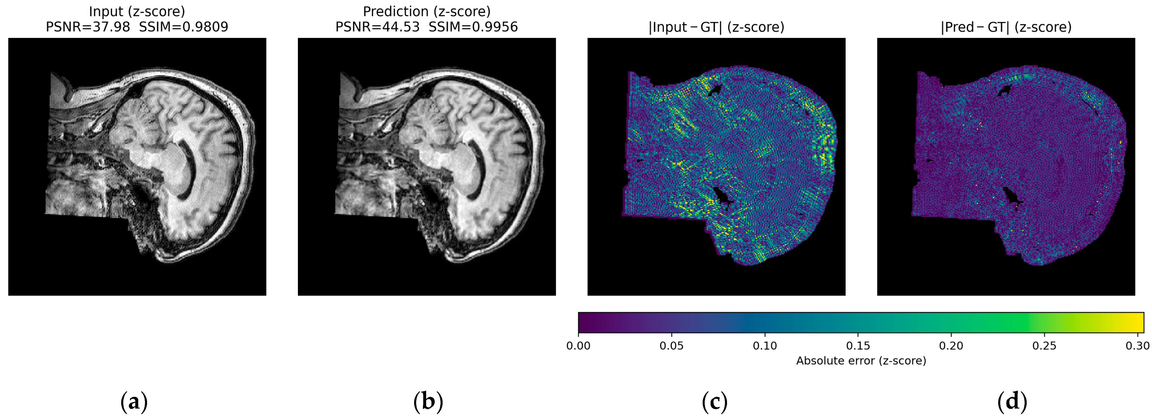
Figure 19.
Ringing artifact suppression (z-score domain). (a) Input image with PSNR/SSIM, (b) model prediction, (c) absolute error map ∣Input—GT∣, and (d) absolute error map ∣Pred—GT∣. The prediction reduces edge-related ringing residuals (PSNR 37.98 → 44.53 dB, SSIM 0.9809 → 0.9956).
Figure 19.
Ringing artifact suppression (z-score domain). (a) Input image with PSNR/SSIM, (b) model prediction, (c) absolute error map ∣Input—GT∣, and (d) absolute error map ∣Pred—GT∣. The prediction reduces edge-related ringing residuals (PSNR 37.98 → 44.53 dB, SSIM 0.9809 → 0.9956).
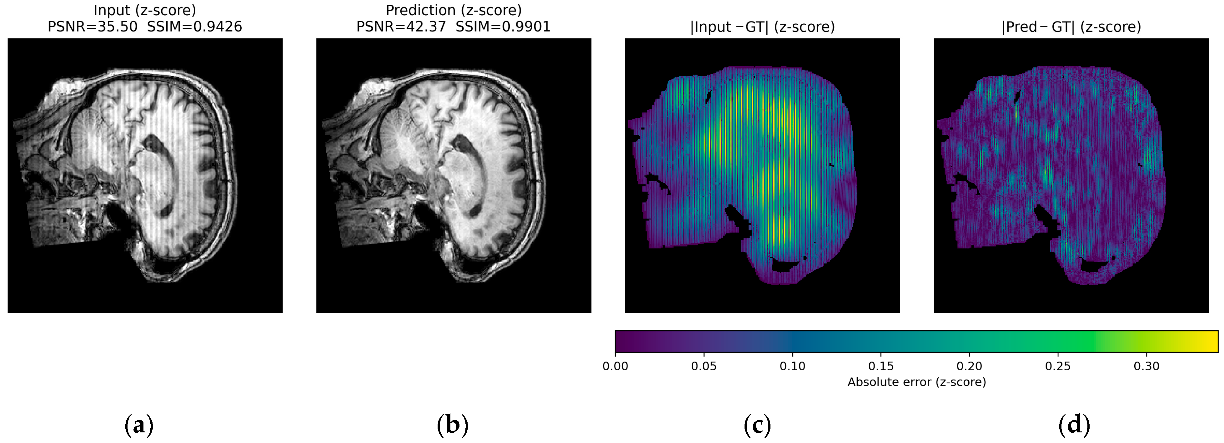
Figure 20.
Herringbone artifact suppression (z-score domain). (a) Input image with PSNR/SSIM, (b) model prediction, (c) ∣Input—GT∣, and (d) ∣Pred—GT∣. The stripe-like residual pattern is markedly attenuated after correction (PSNR 35.50 → 42.37 dB, SSIM 0.9426 → 0.9901).
Figure 20.
Herringbone artifact suppression (z-score domain). (a) Input image with PSNR/SSIM, (b) model prediction, (c) ∣Input—GT∣, and (d) ∣Pred—GT∣. The stripe-like residual pattern is markedly attenuated after correction (PSNR 35.50 → 42.37 dB, SSIM 0.9426 → 0.9901).
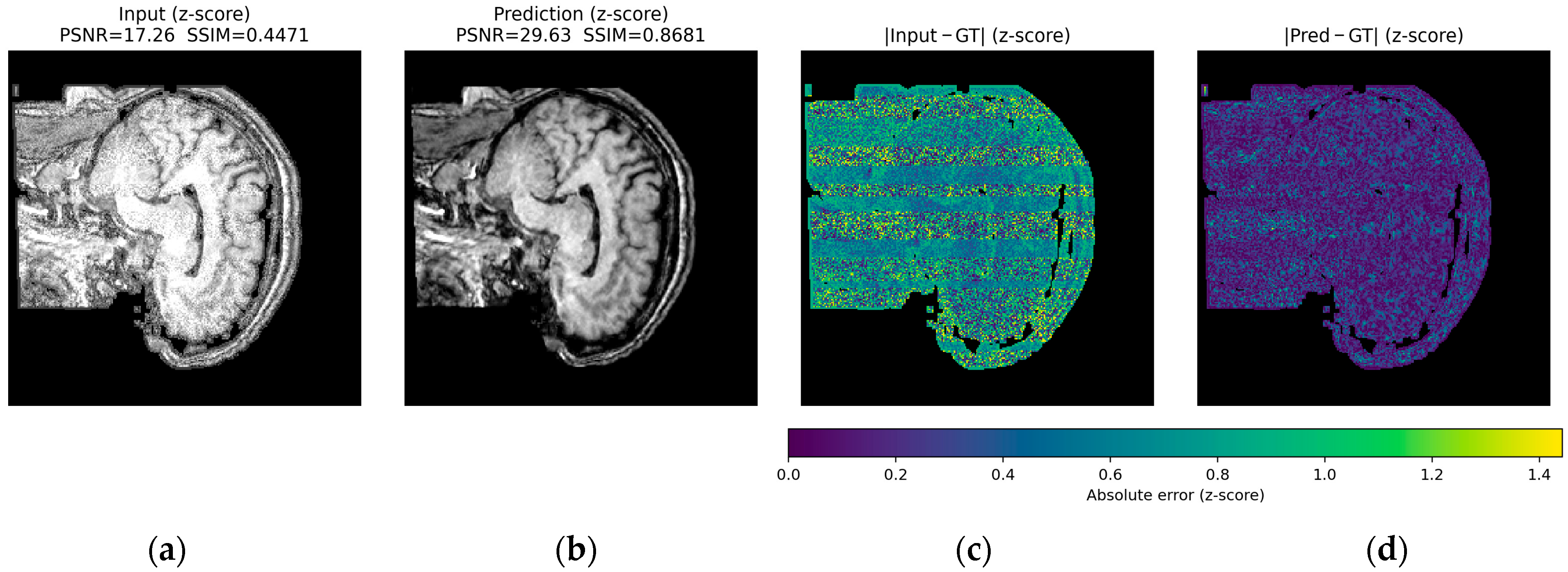
Figure 21.
Zipper artifact suppression (z-score domain). (a) Input image with PSNR/SSIM, (b) model prediction, (c) ∣Input—GT∣, and (d) ∣Pred—GT∣. Strong banding artifacts and large residuals in the input are substantially reduced (PSNR 17.26 → 29.63 dB, SSIM 0.4471 → 0.8681).
Figure 21.
Zipper artifact suppression (z-score domain). (a) Input image with PSNR/SSIM, (b) model prediction, (c) ∣Input—GT∣, and (d) ∣Pred—GT∣. Strong banding artifacts and large residuals in the input are substantially reduced (PSNR 17.26 → 29.63 dB, SSIM 0.4471 → 0.8681).
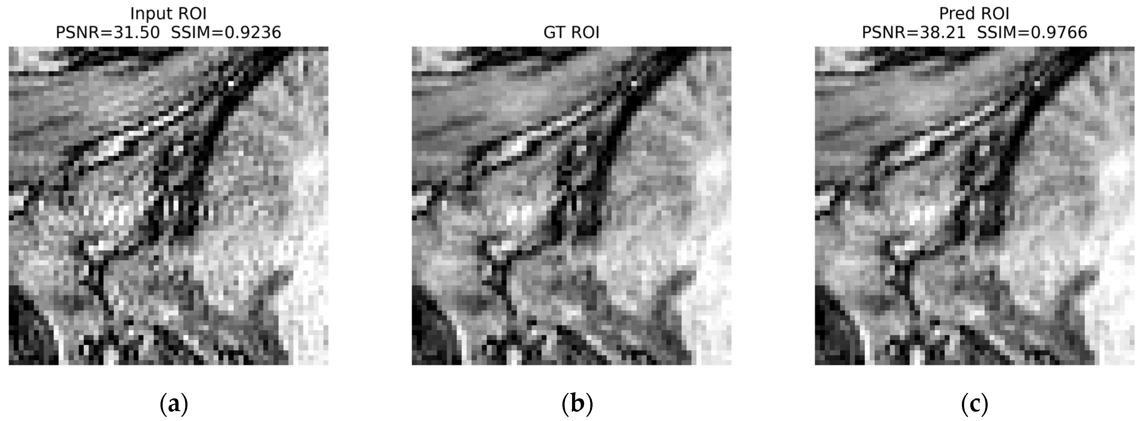
Figure 22.
(a) Input ROI; (b) Ground truth (GT) ROI; (c) Predicted ROI. In the selected ROI, the prediction is closer to the ground truth and reduces ringing-related distortions. Quantitatively, PSNR increases from 31.50 dB to 38.21 dB (+6.71 dB), and SSIM increases from 0.9236 to 0.9766 (+0.0530).
Figure 22.
(a) Input ROI; (b) Ground truth (GT) ROI; (c) Predicted ROI. In the selected ROI, the prediction is closer to the ground truth and reduces ringing-related distortions. Quantitatively, PSNR increases from 31.50 dB to 38.21 dB (+6.71 dB), and SSIM increases from 0.9236 to 0.9766 (+0.0530).
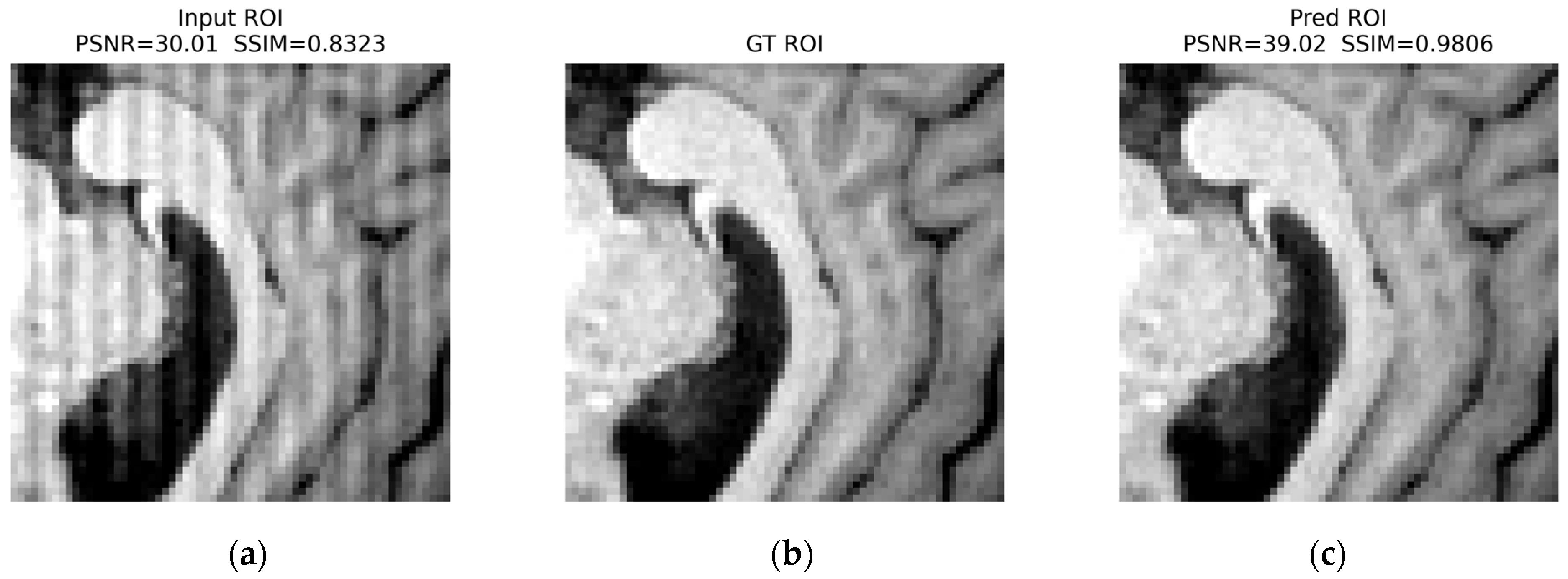
Figure 23.
(a) Input ROI; (b) Ground truth (GT) ROI; (c) Predicted ROI. The ROI shows strong suppression of the stripe-like (herringbone) pattern in the prediction relative to the input, with improved similarity to the GT ROI. PSNR increases from 30.01 dB to 39.02 dB (+9.01 dB), and SSIM increases from 0.8323 to 0.9806 (+0.1483).
Figure 23.
(a) Input ROI; (b) Ground truth (GT) ROI; (c) Predicted ROI. The ROI shows strong suppression of the stripe-like (herringbone) pattern in the prediction relative to the input, with improved similarity to the GT ROI. PSNR increases from 30.01 dB to 39.02 dB (+9.01 dB), and SSIM increases from 0.8323 to 0.9806 (+0.1483).
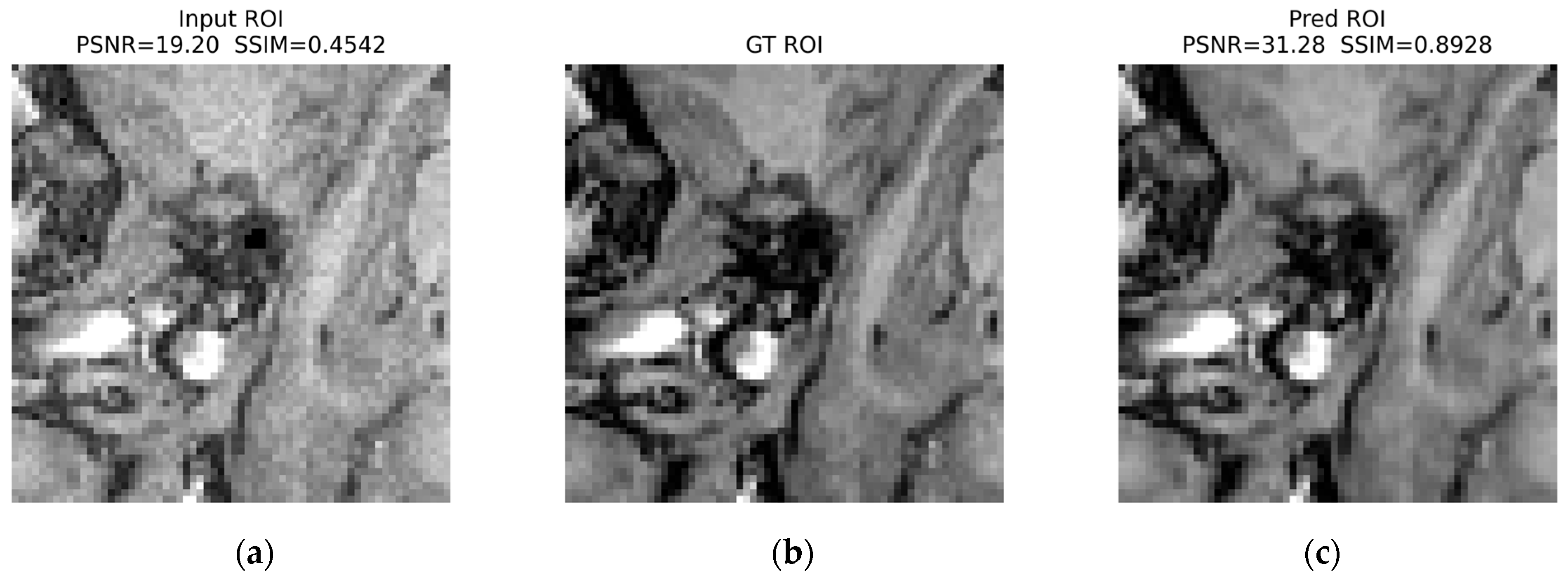
Figure 24.
(a) Input ROI; (b) Ground truth (GT) ROI; (c) Predicted ROI. The prediction substantially reduces pronounced banding within the ROI and restores local contrast toward the GT ROI. PSNR increases from 19.20 dB to 31.28 dB (+12.08 dB), and SSIM increases from 0.4542 to 0.8928 (+0.4386).
Figure 24.
(a) Input ROI; (b) Ground truth (GT) ROI; (c) Predicted ROI. The prediction substantially reduces pronounced banding within the ROI and restores local contrast toward the GT ROI. PSNR increases from 19.20 dB to 31.28 dB (+12.08 dB), and SSIM increases from 0.4542 to 0.8928 (+0.4386).
Table 1.
Summary of deep learning-based approaches for artifact correction in medical imaging, including artifact category, type, principal causes, solution approaches, and key limitations.
Table 1.
Summary of deep learning-based approaches for artifact correction in medical imaging, including artifact category, type, principal causes, solution approaches, and key limitations.
| Category | Field | Content |
|---|
| Sampling, aliasing and truncation | Artifacts | Aliasing, Gibbs, ringing, Wrap-around, reduced spatial resolution |
| Main causes | Signal discretization in space and frequency, Undersampling, k-space truncation, Signal outside the field of view |
| Deep learning solution approaches | CNN/ResNet/autoencoder reconstruction [1,2,3,4,5,9,10,11,12,13,14,15]; zero-shot and in situ adaptation [6,7]; adversarial and dual-domain learning [8]; structured k-space correction [16,17]; model-based unrolling [22,23,24]; transformer reconstruction [31,32,33,34,35]; hybrid pipelines [8,22,23,24,31,32,33,34,35] |
| Identified limitations | Architectural complexity in dual-domain models [8]; limited 3D and low-SNR validation [6,7]; high computational cost [10]; possible suppression of subtle findings [11]; limited pathological validation [12,13,14]; metric shifts under threshold-based evaluation [15]; dependence on training data [16]; latency in iterative methods [36,37,38,39] |
| Motion artifacts | Artifacts | Blurring, ghosting, phase stiffness, respiratory artifacts, motion shifts in DWI |
| Main causes | Voluntary and involuntary patient motion, breathing, fetal motion, cardiac motion |
| Deep learning solution approaches | CNN/U-Net restoration [41,42,43,44,51,52]; GAN-based approaches [45,48,55]; diffusion and score-based models [46,47,54]; unpaired and autoencoder pipelines [50,56]; hybrid motion estimation + restoration [41,42,43,44,45,46,47,50,51,52,53,54,55,56] |
| Identified limitations | GAN instability and possible anatomical artifacts [45]; high computational cost in diffusion models [46,47]; limited multicenter and real-time 3D/4D validation [53]; sensitivity to hyperparameters and limited pathological evaluation [55,56] |
| Off resonance and susceptibility B0 | Artifacts | Geometric distortions, signal voids from metals, signal mismatches, frequency shifts |
| Main causes | B0 field inhomogeneity, susceptibility differences between tissues, metallic implants, and incomplete shimming |
| Deep learning solution approaches | ΔB0-based geometric correction [63,64,65]; CNN/U-Net restoration [3,58,61,62]; unsupervised and multimodal approaches (dual polarity, CT–MRI transfer, GANs) [57,60,62]; hybrid field-map + restoration pipelines [57,58,59,60,61,62,63,64,65] |
| Identified limitations | Additional acquisitions may increase scan time [57]; dependence on reversed polarity data [63]; possible alteration of derived metrics (e.g., FA in TBSS) [62]; training sensitivity to hyperparameters [65]; robustness to motion and protocol variability remains limited [63] |
| Ghosting phase, errors and system effects | Artifacts | Herringbone spike and corduroy patterns, zipper artifacts, ghosting from flow and pulsatility, gradient nonlinearities, eddy currents |
| Main causes | Phase errors, RF interference and unintended RF emissions, system nonlinearities and gradient faults, eddy currents, flow, and pulsatility |
| Deep learning solution approaches | CNN/U-Net restoration [66,68]; coil-combination and subspace methods [63,67]; generative and hybrid approaches for metal/flow artifacts [61,69]; physics-informed pipelines with CNN post-processing [63,66,67,68,69] |
| Identified limitations | Dependence on physical model assumptions [66]; computational cost at high resolution [66]; limited generalization with task-specific annotations [61]; robustness across scanners and protocols still under evaluation [67] |
Table 2.
Parameters for controlling the severity of the ringing artifact.
Table 2.
Parameters for controlling the severity of the ringing artifact.
| Parameter | Lower Limit Value | Higher Limit Value | Type |
|---|
| Scalar intensity ( | 0 | 1 | Decimal |
| Propagation axis | 0 | 2 | Integer |
| End angle () | 0 | 360 | Integer |
| Initial angle () | | | Integer |
| Outer radius () | 118 | 123 | Integer |
| Inner radius () | | | Integer |
Table 3.
Parameters controlling the severity of the herringbone artifact.
Table 3.
Parameters controlling the severity of the herringbone artifact.
| Parameter | Lower Limit Value | Higher Limit Value | Type |
|---|
| Smoothing | 3 | 20 | Integer |
| Propagation axis | 0 | 2 | Integer |
| Selection point | 0 | 3 | Integer |
| Kernel size () | 3 | 13 | Integer |
| Distance | −30 | 30 | Integer |
Table 4.
Parameters for controlling the severity of zipper artifacts.
Table 4.
Parameters for controlling the severity of zipper artifacts.
| Parameter | Lower Limit Value | Higher Limit Value | Type |
|---|
| Intensity | 15 | 50 | Integer |
| Propagation axis | 0 | 2 | Integer |
| Number of artifacts | 1 | 16 | Integer |
| Variability | 20 | 40 | Integer |
| Amplitude | 10 | 50 | Integer |
Table 5.
Hyperparameter values.
Table 5.
Hyperparameter values.
| Parameter | Value |
|---|
| Input/Output Bands | 4 (AA, AD, DA, DD) |
| Encoder/Decoder Levels | 4/4 |
| Loss | WaveletLoss (band-weighted L1) |
| Metrics | SSIM and PSNR (image), MAE per band |
| Optimizer | Adam |
| Batch Size/Epochs | 8/50 |
| Dataloader Workers | 4 |
| Wavelet | db2 |
| Minimum Tile Size | ≥32 × 32 |
Table 6.
Results of multivariate analysis on wavelet + GLCM characteristics in training and validation.
Table 6.
Results of multivariate analysis on wavelet + GLCM characteristics in training and validation.
| Test | Stat | p-Value |
|---|
| Energy Distance | 0.010375 | <0.005 |
| MMD-RBF | 0.000320 | <0.005 |
| Sliced-Wasserstein | 0.073419 | <0.005 |
Table 7.
Results of the wavelet family selection experiment (db1–db6) for brain MRI artifact correction using a U-Net architecture.
Table 7.
Results of the wavelet family selection experiment (db1–db6) for brain MRI artifact correction using a U-Net architecture.
| Wavelet Family | SSIM | MAE |
|---|
| db2 | 0.97322 ± 0.00217 | 0.03570 ± 0.00051 |
| db4 | 0.97306 ± 0.00203 | 0.03535 ± 0.00046 |
| db3 | 0.97180 ± 0.00139 | 0.03552 ± 0.00085 |
| db1 | 0.97149 ± 0.00252 | 0.03721 ± 0.00119 |
| db6 | 0.97068 ± 0.00219 | 0.03541 ± 0.00101 |
| db5 | 0.97049 ± 0.00244 | 0.03641 ± 0.00134 |
Table 8.
Average MSE per wavelet component and overall SSIM and PSNR across the entire image.
Table 8.
Average MSE per wavelet component and overall SSIM and PSNR across the entire image.
| Metric | Art Value | Correction Value |
|---|
| MSE_ | 0.048 ± 0.869 | 0.007 ± 0.009 |
| MSE_ | 0.008 ± 0.011 | 0.003 ± 0.004 |
| MSE_ | 0.009 ± 0.011 | 0.004 ± 0.004 |
| MSE_ | 0.007 ± 0.010 | 0.002 ± 0.003 |
| MSE_ | 0.018 ± 0.029 | 0.004 ± 0.005 |
| PSNR [dB] | 33.42 ± 6.939 | 43.337 ± 5.364 |
| SSIM | 0.938 ± 0.067 | 0.985 ± 0.022 |
Table 9.
Quantitative evaluation of artifact correction and edge preservation (input vs. output).
Table 9.
Quantitative evaluation of artifact correction and edge preservation (input vs. output).
| Metric | | |
|---|
| Edge-PSNR | 38.41 ± 12.39 | 41.04 ± 8.54 |
| Edge-SSIM | 0.952 ± 0.121 | 0.980 ± 0.060 |
| Grad-L1 | 0.0744 ± 0.0530 | 0.0540 ± 0.0392 |
| Grad-L2 | 0.0622 ± 0.0466 | 0.0436 ± 0.0342 |
| Edge Dice/F1 | 0.920 ± 0.0500 | 0.938 ± 0.0416 |
| Radon peak ratio | 6.72 ± 10.33 | 2.89 ± 3.46 |
Table 10.
Stress test on mixed periodic artifacts.
Table 10.
Stress test on mixed periodic artifacts.
| Mixture Artifact | n | PSNR in | PSNR out | SSIM in | SSIM out | ΔPSNR | ΔSSIM |
|---|
| Ringing + zipper | 150 | 17.83 ± 3.00 | 30.61 ± 3.39 | 0.4621 ± 0.1336 | 0.8911 ± 0.0767 | +12.78 | +0.4290 |
| Herringbone + ringing | 150 | 35.13 ± 2.86 | 38.54 ± 2.84 | 0.9600 ± 0.0208 | 0.9793 ± 0.0144 | +3.41 | +0.0192 |
| Zipper + herringbone | 150 | 17.64 ± 3.21 | 29.07 ± 2.88 | 0.3902 ± 0.1557 | 0.8579 ± 0.0668 | +11.43 | +0.4678 |
| Ringing + zipper + herringbone | 150 | 17.58 ± 3.35 | 28.95 ± 2.87 | 0.3950 ± 0.1582 | 0.8570 ± 0.0701 | +11.37 | +0.4620 |
Table 11.
PSNR and SSIM results stratified by artifact severity (input vs. output) by artifact type.
Table 11.
PSNR and SSIM results stratified by artifact severity (input vs. output) by artifact type.
| Artifact | Severity | Severity Interval | n | PSNR in | PSNR out | SSIM in | SSIM out |
|---|
| herringbone | mild | smooth ≤ 6 | 573 | 47.13 ± 2.88 | 47.34 ± 1.65 | 0.9948 ± 0.0031 | 0.9966 ± 0.0017 |
| herringbone | moderate | 6 < smooth < 16 | 2414 | 40.88 ± 3.60 | 44.35 ± 2.68 | 0.9790 ± 0.0132 | 0.9930 ± 0.0069 |
| herringbone | severe | smooth ≥ 16 | 903 | 37.41 ± 3.44 | 42.63 ± 2.60 | 0.9618 ± 0.0176 | 0.9899 ± 0.0096 |
| ringing | mild | intensity ≤ 0.27195 | 1386 | 42.57 ± 5.59 | 45.50 ± 3.91 | 0.9886 ± 0.0121 | 0.9950 ± 0.0048 |
| ringing | moderate | 0.27195 < intensity < 0.76809 | 2038 | 42.39 ± 5.11 | 44.93 ± 3.58 | 0.9896 ± 0.0093 | 0.9950 ± 0.0037 |
| ringing | severe | intensity ≥ 0.76809 | 982 | 40.17 ± 4.56 | 44.24 ± 3.53 | 0.9854 ± 0.0104 | 0.9945 ± 0.0040 |
| zipper | mild | intensity ≤ 22 | 658 | 20.90 ± 1.37 | 35.77 ± 3.59 | 0.6531 ± 0.0468 | 0.9537 ± 0.0321 |
| zipper | moderate | 22 < intensity < 41 | 2579 | 18.49 ± 1.83 | 34.08 ± 3.02 | 0.5267 ± 0.0855 | 0.9384 ± 0.0410 |
| zipper | severe | intensity ≥ 41 | 996 | 17.41 ± 2.03 | 32.04 ± 3.72 | 0.4848 ± 0.0858 | 0.9142 ± 0.0757 |
Table 12.
Quantitative ablation study of the main architecture components.
Table 12.
Quantitative ablation study of the main architecture components.
| Model | SSIM | PSNR |
|---|
| Our model | 0.98528 ± 0.02218 | 43.33710 ± 5.36451 |
| without Radon | 0.98242 ± 0.02441 | 42.65113 ± 5.73252 |
| without Attention | 0.97295 ± 0.04182 | 41.13236 ± 6.58765 |
| without AA component | 0.84215 ± 0.08133 | 34.87268 ± 7.15305 |
| without AD component | 0.95828 ± 0.04865 | 37.92928 ± 5.17067 |
| without DA component | 0.96147 ± 0.04702 | 38.48882 ± 5.56199 |
| without DD component | 0.95989 ± 0.05004 | 38.30767 ± 5.53929 |
| without AA loss | 0.96311 ± 0.04702 | 38.36318 ± 5.26245 |
| without AD loss | 0.96266 ± 0.04576 | 38.05932 ± 4.99527 |
| without DA loss | 0.96354 ± 0.04467 | 38.21393 ± 5.06365 |
| without DD loss | 0.96377 ± 0.04325 | 38.17828 ± 4.85161 |
Table 13.
Average SSIM and PSNR results for each trained model compared with the proposed approach.
Table 13.
Average SSIM and PSNR results for each trained model compared with the proposed approach.
| Model | SSIM | PSNR |
|---|
| Our model | 0.98528 ± 0.02218 | 43.33710 ± 5.36451 |
| U-Net | 0.97295 ± 0.04182 | 41.13236 ± 6.58765 |
| GAN | 0.97390 ± 0.03990 | 41.08036 ± 6.32473 |
| Spatial + channel attention | 0.97353 ± 0.03422 | 41.41551 ± 6.70846 |
| Attention–attention | 0.93782 ± 0.04089 | 32.84799 ± 3.70444 |
| Vision transformer | 0.97322 ± 0.04279 | 40.77219 ± 6.18026 |
Table 14.
Computational cost comparison across the different approaches.
Table 14.
Computational cost comparison across the different approaches.
| Model | Params (M) | FLOPs/
MACs (G) | Peak GPU Mem (GB) | Train Time
/Epoch (s) | Total Train Time (min, 100 ep) | Inference
Latency/Slice (ms) |
|---|
| Our model | 33.482 | 14.337 | 1.433 ± 0.03 | 359.83 ± 10.79 | 599.72 ±17.99 | 5.461 ± 0.27 |
| U-Net | 31.391 | 13.933 | 1.582 ± 0.03 | 335.07 ± 10.05 | 558.45 ± 16.75 | 4.399 ± 0.22 |
| GAN | 34.155 | 13.933 | 1.583 ± 0.04 | 671.05 ± 26.84 | 1118.42 ± 44.74 | 4.389 ± 0.22 |
| Spatial + channel attention | 32.177 | 14.451 | 4.554 ± 0.09 | 601.78 ± 24.07 | 1002.97 ± 40.12 | 6.202 ± 0.37 |
| Attention–attention | 3.599 | 9.881 | 4.528 ± 0.09 | 4324.75 ± 216.24 | 7207.92 ± 360.4 | 23.526 ± 1.41 |
| Vision transformer | 43.508 | 14.442 | 1.968 ± 0.04 | 529.47 ± 21.18 | 882.44 ± 35.30 | 12.327 ± 0.74 |




 ,
,