The Role of Radiomic Analysis and Different Machine Learning Models in Prostate Cancer Diagnosis

Abstract

Prostate cancer (PCa) is the most common malignancy in men. Precise grading is crucial for the effective treatment approaches of PCa. Machine learning (ML) applied to biparametric Magnetic Resonance Imaging (bpMRI) radiomics holds promise for improving PCa diagnosis and prognosis. This study investigated the efficiency of seven ML models to diagnose the different PCa grades, changing the input variables. Our studied sample comprised 214 men who underwent bpMRI in different imaging centers. Seven ML algorithms were compared using radiomic features extracted from T2-weighted (T2W) and diffusion-weighted (DWI) MRI, with and without the inclusion of Prostate-Specific Antigen (PSA) values. The performance of the models was evaluated using the receiver operating characteristic curve analysis. The models’ performance was strongly dependent on the input parameters. Radiomic features derived from T2WI and DWI, whether used independently or in combination, demonstrated limited clinical utility, with AUC values ranging from 0.703 to 0.807. However, incorporating the PSA index significantly improved the models’ efficiency, regardless of lesion location or degree of malignancy, resulting in AUC values ranging from 0.784 to 1.00. There is evidence that ML methods, in combination with radiomic analysis, can contribute to solving differential diagnostic problems of prostate cancers. Also, optimization of the analysis method is critical, according to the results of our study.

1. Introduction

Prostate cancer (PCa) is the second-most common cancer in men worldwide and the fifth leading cause of cancer-related deaths among men [1]. The early detection and grading of PCa play a crucial role in patient management, therapy planning, and long-term survival evaluation. Serum Prostate-Specific Antigen (PSA) and Digital Rectal Examination (DRE) are the most widely used PCa screenings in clinical practice, following the European Association of Urology (EAU)—European Society for Radiotherapy and Oncology (ESTRO)—International Society of Geriatric Oncology (SIOG) Guidelines [2]. The traditional PSA cutoff of 4 ng/mL imposes histopathological verification through biopsy [3,4]. However, the study by Marriel et al. indicates that PSA has a low specificity of 20%, disputing the usefulness of PSA in the accurate diagnosis of clinically significant prostate cancer (cs-PCa), since they recorded many cases with low PSA value and cs-PCa and, contrarily, high PSA value in benign pathologies like prostate hypertrophy [5].

In the studies of Gershmann et al., only approximately 18% of men with elevated PSA were diagnosed with cancer. The remaining 82% of men underwent biopsies without actually having prostate cancer and were exposed to potential complications such as bleeding, infection, and urinary retention [6]. Thus, there is a need to develop an algorithm that, by taking clinical, demographic, and imaging information, will more accurately define the cases that truly need a biopsy [7].

Multiparametric Magnetic Resonance Imaging (mpMRI) can be considered a sophisticated diagnostic approach for the detection, differentiation, and risk classification of PCa since it provides imaging biomarkers from conventional and advanced imaging techniques, such as high-resolution T2-weighted (T2W), diffusion-weighted (DWI) and dynamic contrast-enhanced sequences (DCE) [8,9]. Mp-MRI diagnostic accuracy in PCa further increased the area under the receiver operating characteristic curve (AUC = 0.893) value when expert radiologists followed the Prostate Imaging Reporting and the Data System Version 2 (PI-RADS v2), which is considered the most promising approach for PCa screening with high diagnostic accuracy AUC = 0.893 to PCa differentiation [10].

The lack of expert prostate imaging radiologists and the interobserver variability in the interpretation of mp-MRI, the large spectrum of acquisition parameters, and the heterogeneity of PCa tumors are factors that significantly reduce the sensitivity and specificity of the imaging method [11,12,13].

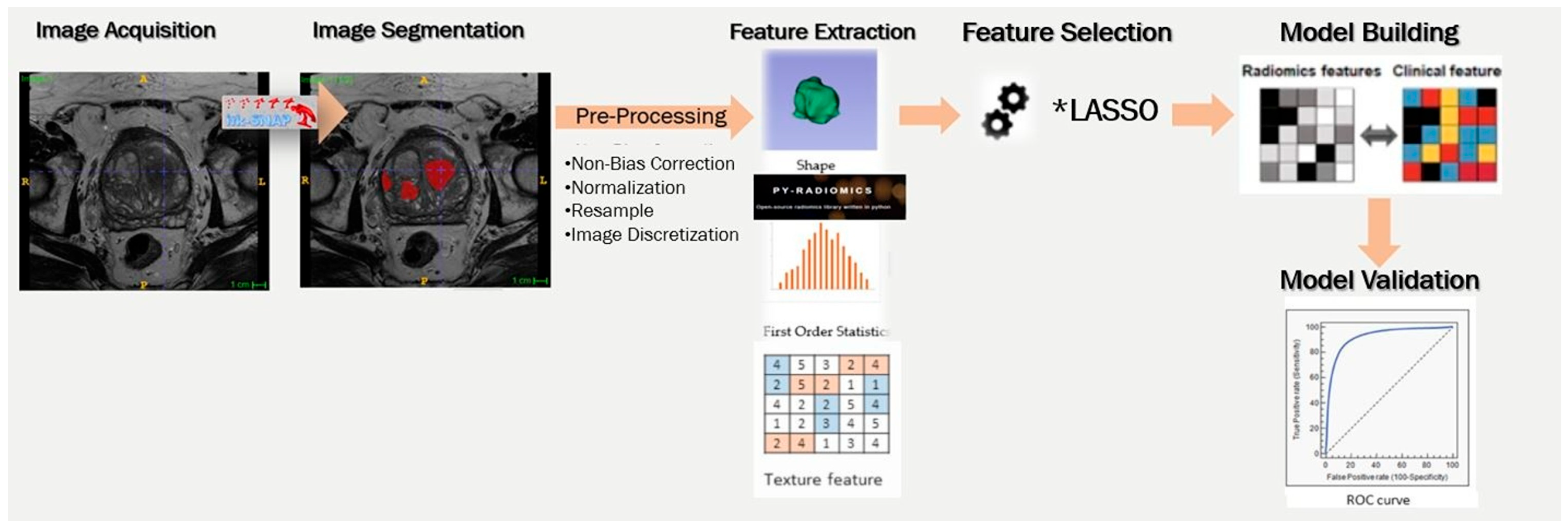
Consequently, there is a need for objective indices to mitigate radiologists’ faults. Radiomic analysis and machine learning (ML) methods offer an objective approach for evaluating MRI data by extracting imaging features usually not easily detectable by the radiologist’s eye [14,15]. Radiomic analysis allows the mining of quantitative characteristics like texture, size, and shape from clinical images, like MRI, useful to diagnose and differentiate PCa [14]. ML is adept at analyzing vast, complex datasets without prior biomedical hypotheses, uncovering insights that may be clinically relevant. As a result, ML, particularly in the area of classification, is being integrated into radiomic research to refine prostate cancer evaluations and reduce subjectivity [16]. Although ML and radiomics combined are promising diagnosis tools in prostate cancer, they face limitations related to the high susceptibility to variations in acquisition parameters, the sample size, the statistical methodological approach, and the heterogeneous datasets mixing peripheral zone (PZ) with transition zone (TZ) tumors [17].

The main purpose of this study was to evaluate the diagnostic performance of different ML approaches to detect and assess PCa aggressiveness using standardized MRI protocol across many centers. In particular, we investigated the diagnostic performance of ML to differentiate the different PCa grades by (a) applying seven ML models and (b) changing the input variables.

2. Materials and Methods

2.1. Patient Population

Our sample size consisted of 214 participants with increased PSA or clinical symptoms related to prostate dysfunction who underwent MRI examination in three different imaging centers equipped with four different MRI systems. The data comprised four datasets: dataset 1 (86 exams on a 3T MRI), dataset 2 (21 exams on a 1.5 T MRI), dataset 3 (88 exams on a 3 T MRI), and dataset 4 (19 exams on a 1.5T MRI). All participants were given Τransrectal Ultrasound Guided (TRUS) biopsy in order to validate the lesion type.

Exclusion criteria were (1) prior therapy history for PCa patients, including antihormonal therapy, radiation, cryotherapy, or prostatectomy, (2) incomplete information or (3) severe imaging artifacts of the MRI images, and (4) lack of serum PSA level.

2.2. MRI Acquisitions

The image acquisition protocol was harmonized across all centers since the core scientific group had set minimum requirements, such as high-resolution T2W images of at least 3.0 mm gapless slice distance in the axial plane and DWI images with the same slice distance, 2 b values with the high b value at least 1000 s/mm².

2.3. MRI Lesion Segmentation

All individual lesions were manually delineated on T2W based on PI-RADSv2.1 reports by an expert radiologist with ten years of experience in examining PCa lesions using ITK-SNAP [18].

2.4. Image Pre-Processing

Firstly, we applied Bias correction on T2W and DWI images to compensate for intensity non-uniformities using N4 Bias Correction on SimpleITK Python 2.1.1.2 library [19]. Then, we performed basic normalization by scaling and shifting the values of the whole image to a mean signal value of 300 and a standard deviation of 100 [12]. Finally, a resampling pixel sampling 1 × 1 × 1 mm³ with sitkBSpline interpolator and fixed bin-width (FBW) discretization equal to 10 for T2W images and 5 for DWI images were performed to handle differences in image resolution [20,21]. All the pre-processing steps were applied using the open-source software Pyradiomics v1.3.0 [22].

2.5. Feature Extraction

Radiomic features were extracted from the pre-processed T2W and DWI images using the Pyradiomics v1.3.0, following the Imaging Biomarkers Standardization Initiative (IBSI) processing protocol [22,23]. In particular, in the extracted texture features were included (i) shape-based features (n = 14), (ii) first-order features (n = 18), (iii) gray-level co-occurrence matrix (GLCM) (n = 22) features, (iv) gray-level size zone matrix (GLSZM) features (n = 19), (v) gray-level run length matrix (GLRLM) features (n = 14), and (vi) gray-level dependence matrix (GLDM) features (n = 14). These features are enabled in the Pyradiomics code by default. Appendix A includes more details about extracted features. Before proceeding to the next steps, the Radiomics Quality Score (RQS) checklist was applied to ensure the methodological quality of the radiomics study and to enhance the generalizability of our model, achieving a score of 70%. (25/36 of total score) [20,24,25].

2.6. Feature Selection and Dimension Reduction

All radiomics features were normalized before feature selection, with Z scores standardized to eliminate features’ distortions in the range of values [26]. Radiomic approaches generate many features, leading to a high-dimensional dataset. The high dimensionality diminishes the classifier’s performance. In this study, the Gini index algorithm-based feature is selected [27]. The feature selection and dimension reduction were applied by the Orange Data Mining tool (v.3.36.1) [28].

2.7. Model Development

Seven algorithms, K-Nearest Neighbors (k-NN), Naive Bayes (NB), logistic regression (LR), Support Vector Machine (SVM), Decision Tree (DT), Random Forest (RF) and Neural Network (NN), were chosen as classifiers in the classification model analysis of this study. The Orange Data Mining tool (v.3.36.1) was employed in the development of the above machine learning models [28]. The best-performing parameters of classifiers are generally selected for our model development.

The k-NN was set to 6 neighbors per datapoint, Euclidean distance metric with uniform weight distribution [29]. Appendix B justifies the set of k = 6. The NB algorithm was used without any parametric changes. The regularization for LR was set to Least Absolute Shrinkage and Selection Operator (LASSO)-L1 regularization [30]. The SVM type was applied with Cost (C) = 1 and Regression Loss Epsilon (ε) = 0,10, Polynomial Kernel and iteration limit was set to 100, and numerical tolerance to 0.0010. The DT was binary induced with a minimum of 3 instances in leaves, minimum splitting of subsets up to 2 with a maximum tree depth of 200 [31]. The RF had 10 trees with a minimum split of subsets up to 5 [31]. NN contained 3 hidden layers with 100 neurons per hidden layer, 100 maximum number of iterations, and a Rectified Linear Unit (ReLU) activation function [32].

2.8. Performance Evaluation

The performance of ML classifiers was evaluated using the AUC on 10 cross-validation. The validation performance of the algorithms was compared by receiver operating characteristic (ROC) curve analysis. These attributes were computed by default in the Orange Data Mining tool (v.3.36.1) for classification models [28].

Additionally, a held-out test set validation was conducted by using datasets 1, 2, and 3 for training, while dataset 4 was reserved as a test set, allowing for a more thorough evaluation of the models’ generalization performance. This was only applied to the model that differentiated benign from malignant prostate lesions regardless of their location, since dataset 2 and 4, which could be used for a test set, included a limited number of cases with a lesion in the PZ.

The DeLong test was applied to compare the performance of classifiers by testing whether the difference between their area under the curve (AUC) values is statistically significant, using Python 3.9 Software [33].

A schematic representation of the pipeline process followed in this study is illustrated in Figure 1.

3. Results

3.1. Clinical Characteristics

One hundred thirteen participant patients (53%) were diagnosed with benign lesions, and the remaining 101 (47%) with malignant lesions. In particular, biopsy showed a Gleason score (GS) ≤ 6 in 113 patients (53%) and a GS > 6 in 101 patients (47%). The international Society of Urological Pathology (ISUP) group was distributed in the low-risk group (ISUP = 1) in 113 (52.80%) patients, in the intermediate-risk group (ISUP = 2 and ISUP = 3) in 83 (38.79%) patients, and in the high-risk group (ISUP > 3) in 18 (8.41%) patients. The most lesions were detected in PZ in 158 (74%) patients, and the other 56 (26%) lesions were located in οther prostate zones. Further details on patient clinical characteristics can be found in

Table 1. Clinical and epidemiological characteristics of patient cohort.

Variable
No. of patients	214
Benign	113
Malignant	101
Median age (y) (mean ± std)	66.00 ± 7.77
Median PSA level (ng/mL) (mean ± std)	8.06 ± 7.03
Median prostate volume (mm3) (mean ± std)	61.17 ± 40.28
Histopathologically confirmed lesions	214
Gleason score (GS)
GS < 6	62
GS = 6	51
GS = 7 (3 + 4)	46
GS = 7 (4 + 3)	37
GS > 7	18
International Society of Urological Pathology (ISUP) group
ISUP = 1	113
SUP = 2	46
ISUP = 3	37
ISUP = 4	11
ISUP = 5	7
Lesion location
Peripheral zone	158
Other zones	56

.

3.2. Predictive Ability of Differentiation of Benign and Malignant Prostate Lesions

Firstly, the dataset was grouped based on GS of lesion, independent of lesion location. Class A included benign prostate lesions (GS $\le$ 6), and Class B malignant prostate lesions (GS > 6). The different AUC results of all the models used for T2W dataset, DWI dataset, and their combination are presented in

Table 2. Area under curve (AUC) results across different datasets and algorithms, evaluated under various discrimination criteria, for both the entire prostate gland and the peripheral zone.

		Entire Prostate	Peripheral Zone
	Discriminate Criterion	$\mathbf{GS}* \le$ 6 vs. GS > 6	ISUP* 2 vs. ISUP 3	ISUP* 1 vs. ISUP 2&3
Algorithm Models	Features	AUC	AUC	AUC
Random Forest	T2W*	0.747	0.670	0.739
	DWI*	0.711	0.762	0.670
	T2W + DWI	0.735	0.709	0.603
	T2W + DWI + PSA*	0.946	0.995	0.995
kNN	T2W	0.738	0.545	0.756
	DWI	0.721	0.713	0.606
	T2W + DWI	0.726	0.632	0.599
	T2W + DWI + PSA	0.868	0.784	0.898
Naive Bayes	T2W	0.763	0.726	0.746
	DWI	0.728	0.686	0.688
	T2W + DWI	0.786	0.725	0.675
	T2W + DWI + PSA	0.830	0.921	0.975
Logistic Regression	T2W	0.755	0.736	0.746
	DWI	0.719	0.710	0.622
	T2W + DWI	0.807	0.738	0.616
	T2W + DWI + PSA	0.884	0.972	1.000
SVM	T2W	0.717	0.369	0.750
	DWI	0.703	0.845	0.545
	T2W + DWI	0.736	0.715	0.647
	T2W + DWI + PSA	0.957	1.000	1.000
Decision Tree	T2W	0.721	0.582	0.747
	DWI	0.630	0.634	0.553
	T2W + DWI	0.678	0.609	0.678
	T2W + DWI + PSA	0.953	0.962	1.000
Neural Network	T2W	0.753	0.597	0.760
	DWI	0.703	0.824	0.569
	T2W + DWI	0.726	0.769	0.651
	T2W + DWI + PSA	0.992	0.989	0.989

*- GS*, Gleason score; ISUP*, International Society of Urological Pathology; T2W*, T2-weighted; DWI*, diffusion-weighted; PSA*, Prostate-Specific Antigen.

.

Table 3. p-values from Pairwise DeLong test, which assesses whether the differences in (area under curve) AUC between pairs of models are statistically significant for different classification tasks.

Delong t-Test, p-Values (GS* ≤ 6 vs. GS* > 6)
Model 1/Model 2	NB*	kNN*	LR*	SVM*	DT*	RF*	NN*
NB*	-	0.6231	0.0144	0.0000	0.0188	0.0003	0.0005
kNN	0.0623	-	0.0392	0.0000	0.0311	0.0003	0.0005
LR*	0.0014	0.0392	-	0.0005	0.7591	0.1472	0.0018
SVM*	0.0000	0.0000	0.0005	-	0.0023	0.0332	0.0005
DT*	0.0019	0.0311	0.7591	0.0023	-	0.3381	0.0321
RF*	0.0000	0.0003	0.1472	0.0332	0.3381	-	0.0045
NN*	0.0005	0.0018	0.0005	0.0005	0.0321	0.0045	-
Delong t-test, p-values (ISUP* 2 vs. ISUP* 3)
Model 1/Model 2	NB*	kNN	LR*	SVM*	DT*	RF*	NN*
NB*	-	0.0219	0.0501	0.0194	0.0426	0.0082	0.0445
kNN	0.0219	-	0.1028	0.0021	0.1221	0.0155	0.4658
LR*	0.0501	0.1028	-	0.0652	0.9284	0.5712	0.0489
SVM*	0.0194	0.0021	0.0652	-	0.0781	0.1449	0.0187
DT*	0.0426	0.1221	0.9284	0.0781	-	0.6358	0.0018
RF*	0.0082	0.0155	0.5712	0.1449	0.6358	-	0.0189
NN*	0.0445	0.4658	0.0489	0.0187	0.0018	0.0189	-
Delong t- tets, p-values (ISUP* 1 vs. ISUP* 2,3)
Model 1/Model 2	NB*	kNN*	LR*	SVM*	DT*	RF*	NN*
NB*	-	0.5420	0.0368	0.0012	0.0031	0.0058	0.0248
kNN	0.5420	-	0.0793	0.0007	0.0020	0.0045	0.0048
LR*	0.0368	0.0793	-	0.0180	0.0736	0.1199	0.0112
SVM*	0.0012	0.0007	0.0180	-	0.0643	0.1161	0.0187
DT*	0.0031	0.0020	0.0736	0.0643	-	0.8378	0.0287
RF*	0.0058	0.0045	0.1199	0.1161	0.8378	-	0.0385
NN*	0.0248	0.0048	0.0112	0.0187	0.0287	0.0385	-

*.NB*, Naïve Bayes; kNN*, k-Neural Network; LR*, logistic regression; SVM*, Support Vector Machine; *DT, Decision Tree; RF*, Random Forest, *NN: Neural Network; GS*, Gleason score; ISUP*, International Society of Urological Pathology.

presents the statistical comparison of AUCs between models using the DeLong test to assess the significance of performance differences.

Model performance based on held-out cross-validation is presented in

Table 4. Results of held-out cross validation by using datasets 1, 2, and 3 for training and dataset 4 as the test set, incorporating T2W, DWI, and PSA as input features. The classification task was based on a Gleason score discrimination cut-off of 6, distinguishing benign (GS ≤ 6) from malignant (GS ≥ 7) prostate lesions.

Algorithm	Random Forest	kNN	Naïve Baiyes	Logistic Regression	SVM	Decision Tree	Neural Network
Evaluation method	Area under curves (AUC) values
Cross-validation	0.946	0.868	0.830	0.884	0.957	0.953	0.992
Held-out set	0.814	0.764	0.700	0.764	1.000	0.929	0.936

.

3.3. Predictive Ability of Differentiation of Low-Risk Lesions from Intermediate-Risk Lesions on the Peripheral Zone

The dataset was divided based on the ISUP score of lesions that were located in the PZ of the prostate gland. Class A included low-risk lesions with ISUP = 1 (GS = 6), and Class B intermediate-risk lesions with ISUP = 2 (GS = 3 + 4) and ISUP = 3 (GS = 4 + 3). AUC values of various ML models across different datasets are presented in Table 2.

3.4. Predictive Ability of Differentiation of ISUP = 2 and ISUP = 3 on the Peripheral Zone

The dataset was divided into classes based on the ISUP score of lesions located in the peripheral zone (PZ) of the prostate gland. Class A included lesions with ISUP = 2, and Class B lesions with ISUP = 3. AUC results across different datasets and all the models are presented in Table 2, and the corresponding ROC curve is illustrated in Figure 2.

4. Discussion

The past decade, the research community has stratified post-processing methods such as radiomic analysis combined with ML models to diagnose clinically significant prostate cancer. In this study, we validated the noteworthy contribution of radiomics, trying to reveal the impact of different methodological approaches in the final model’s efficiency. Specifically, we investigated the effect of the different inputs in ML models and the effect of the applied ML methods in different clinical queries.

Our results have shown that the models’ efficiency is highly dependent on the input variables, as expected. In most of the examined scenarios, the T2W and DWI-weighted-derived radiomics either as independent or combined inputs shown limited clinical usability. The models’ efficiency was significantly improved by introducing PSA clinical index independently of lesion location or the degree of malignancy.

The positive effect of introducing a clinical variable on the model performance is in line with the existing literature. Marvaso et al. created four different models. Model 1, including only clinical variables (PSA, pre-operative GS, ISUP, Tumor Nodule Metastasis (TNM) stage and age), achieved AUC = 0.68. Model 2 combined the aforementioned clinical and radiological features (ADC, PI-RADS, lesion volume) and showed a significant improvement, with an AUC of 0.79. Model 3, which integrated prior clinical data with radiomic features, achieved an AUC of 0.71. Finally, Model 4, which combined all features, achieved the highest AUC of 0.81, indicating that the most accurate predictions of PCa pathology were obtained when all variables were incorporated [34].

Similar results were observed in the study by Dominguez et al., where an LR classifier was used to distinguish clinical insignificant (ciPCa) and csPCa, and its performance was improved notably with the inclusion of both radiological (T2W- and Apparent Diffusion Coefficient (ADC)-derived radiomics, prostate volume) and PSA clinical feature (CL) [35]. Specifically, the individual variables, CL, T2W, ADC showed AUC 0.76, 0.85, and 0.81, respectively, and their combination 0.91 [35].

Controversially, there are studies in which the integration of PSA with radiologically derived quantitative metrics did not contribute to further increasing and in some cases decreasing the model’s rendering. In the study conducted by Gong et al., the addition of PSA to the T2W-DWI yielded restricted improvement in model performance. Specifically, the clinical model achieved AUCs of 0.723, while the T2W-DWI model reached 0.788, and the combined T2W-DWI-clinical model slightly improved to 0.780 [36].

However, Lu et al. compared multiple models for PCa prediction in a validation cohort, where the TZ-PSA density model yielded a relatively low AUC of 0.592. In contrast, radiomic models with the ADC-based radscore reaching 0.779, the T2W-based radscore 0.808, the fusion radscore 0.844, and the radiomic nomogram incorporating TZ volume achieving the highest AUC of 0.872. This discrepancy may be attributed to differences in dataset composition (57.4% of their cases located in ΤΖ) [37].

Moreover, there are numerous studies including only radiological metrics in their models and achieving palatable efficiency. A recent review of Antonil et al. presented 14 studies that introduced only radiological features in computational models to discriminate cs-PCa and ciPCa. In line with our results, efficiency was improved when they were introduced to more than one source of feature (in most cases T2w and DWI). AUC ranged from 0.68 to 0.81 when DWI or T2w imaging data were introduced as individual inputs, while their combination achieved AUC 0.73 to 0.98 [38].

Our AUC values were observed to be lower than those reported by some studies in the literature. We assume that this is because most studies used data from a single MR system and applied higher, more sensitive to lesion detection b-values than ours. For example, Jin et al. used b = 2000 s/mm², Jing et al. b = 1500 s/mm², and Hamm et al. b = 1400 s/mm²—all acquired on 3T scanners. A notable exception is Castillo et al., who used data from both 1.5T and 3T systems with b-values ranging from 600 to 1000, reporting an AUC of 0.72, similar to our results [39,40,41,42].

The selection of ML algorithm in PCa classification depends on data characteristics like data dimensionality, feature correlations, and computational resources. Performance evaluation through cross-validation and performance metrics is crucial to determine the most suitable algorithm [43]. The comparison of seven ML algorithms in this survey provides greater reliability for our model.

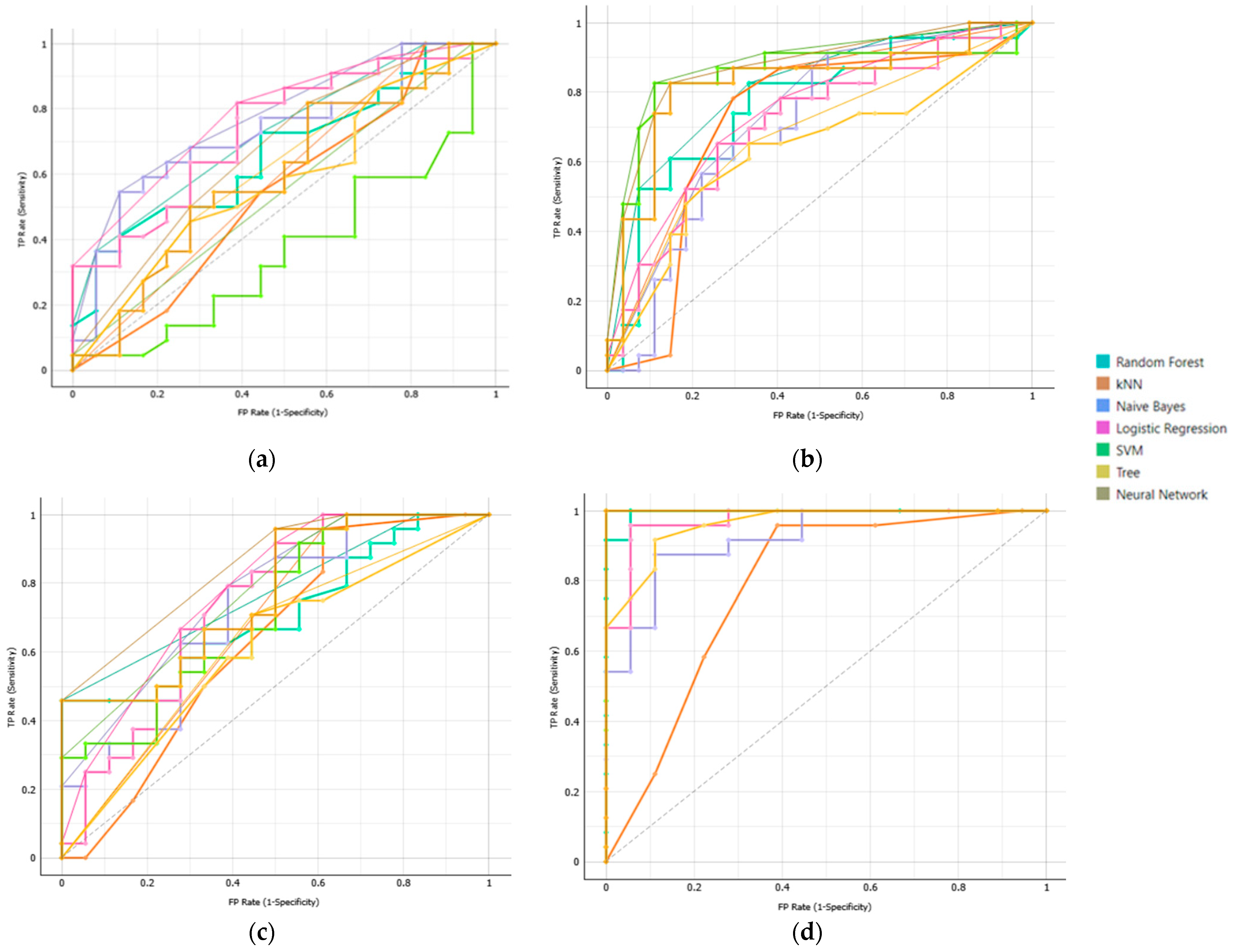
Classification performance of our ML models in the prediction of csPCa was shown to be improved, incorporating T2W, DWI and PSA. Among models, NN achieved the highest performance (AUC = 0.992), followed by SVM (AUC = 0.957), DT (AUC = 0.953), and RF (AUC = 0.946). The efficiency of these models was consistent across different clinical questions posed, highlighting their robustness and generalizability compared to the traditional ML models LR, kNN, and NB, whose performance varied across different tasks. Specifically, LR and kNN showed moderate performance AUC = 0.884 and 0.868, respectively, whereas NB had the lowest performance (AUC = 0.830).

The models’ generalization performance approved relatively consistently across the various evaluation strategies employed, including cross-validation and a held-out validation set. NN exhibited the highest performance during model development, achieving an AUC of 0.992 in cross-validation. Its performance on the held-out set remained robust (AUC = 0.936), indicating strong generalization during initial validation. Similarly, SVM presented a perfect AUC of 1.000 on the held-out set and high performance of AUC = 0.957 in cross-validation. RF and DT delivered strong results during cross-validation (AUCs of 0.946 and 0.953, respectively). While their performance saw a drop on the held-out set (AUCs of 0.814 and 0.929), they still exhibited solid generalization. In contrast, LR, kNN, and NB presented moderate performance during model development (AUC_cross_validation, kNN:0.868; NB: 0.830 and LR: 0.884). However, they maintained consistent performance across datasets (AUC_held_out, kNN: 0.764; NB: 0.700; LR: 0.764) These findings indicate the high predictive abilities of deep learning models compared with traditional ML models, which have less capture ability to detect complex feature interactions.

According to Nematollahi et al. and other related studies, the performance of various supervised ML models using mpMRI or bpMRI data for prostate cancer (PCa) diagnosis varies considerably [31]. Across the published studies different methodological approaches were observed, as regards to the input variables, data sample, and pre- and post-processing analysis steps. Therefore, logistic regression (LR) consistently demonstrates strong performance, with reported AUCs ranging from 0.82 to 0.97 [31]. SVM also perform well, with AUCs between 0.727 and 0.89 for mpMRI and up to 0.85 for bpMRI [38,44,45]. kNN achieves AUCs of 0.82–0.88 (mpMRI) and up to 0.84 (bpMRI), while RF shows AUCs ranging from 0.76 to 0.94 [38,46,47,48]. NB, although still effective, presents the lowest AUCs overall (0.80–0.83 in mpMRI and 0.695–0.80 in bpMRI) [37,48,49]. NN, DT, and LR models using bpMRI yield AUCs ranging from 0.71 to 0.936, depending on the study and configuration [38,43,48,50,51,52,53,54]. The literature review and the results of our study indicate the need to optimize the analysis process, regarding input variables and model choice and the need to standardize the pre-processing analysis steps.

Differentiating ciPCa from csPCa represents an initial critical step in PCa management. However, within the csPCa spectrum, accurate grading—especially the distinction between ISUP grades 1, 2, and ≥3—is essential because it significantly influences treatment strategies. [55] ISUP grade 1 (GS 6, 3 + 3) is often suitable for active surveillance, while ISUP grade 2 (GS 7, 3 + 4) may necessitate treatment for its limited aggressiveness, and ISUP grade ≥ 3 denotes more aggressive disease that warrants immediate intervention [56]. Accurate risk stratification is therefore essential to prevent both overtreatment of low-risk cases and under-management of potentially aggressive disease [57].

A significant disparity exists in PCa research concerned more with detection methods than with the grading and management of low-grade tumors. Twilt et al. observed that only a minority of studies employ ML for ISUP grade prediction using radiomic features. Algorithms’ efficiency to detect high-grade lesions ISUP ≥ 4 is usually high, while that to distinguish intermediate from low-grade lesions is not consistent across studies [58]. Indicatively, Abraham et al., applying a Convolution Neural Network (CNN) to T2W-, DWI-, and ADC-derived metrics, reported low AUC values, especially in low-grade lesions [AUC: 0.626 (GS 6~ISUP = 1), 0.535 (GS 3 + 4~ISUP = 2), 0.379 (GS 4 + 3~ISUP = 3), 0.761 (GS 8~ISUP = 4), and 0.847 (GS ≥ 9~ISUP = 5)] [59]. Low efficiencies were also reported by McGarry et al., who combined four MRI contrasts (T2W, ADC 0–1000, ADC 50–2000, and DCE) to generate Gleason probability maps, achieving low AUC (0.56) for distinguishing GS 4–5 from GS 3, but higher performance (AUC = 0.79) for benign vs. malignant classification [60]. Improved performance was reported by Chaddad et al. in two different studies, where they used two different methodological approaches to lesion grading. At first, they used Joint Intensity Matrix and Gray-Level Co-Occurrence Matrix features from The Cancer Imaging Archive (TCIA) dataset and reported lower than their expectation AUC values of 78.4% (GS ≤ 6), 82.35% (GS 3 + 4), and 64.76% (GS ≥ 4 + 3), which they attribute to omission of key clinical and morphological features [61]. Later, they applied an RF classifier with zone-based features achieving better AUC value in low-grade lesions and high-grade lesions (GS 6 AUC = 0.83 and GS ≥ 4 + 3 AUC = 0.77, respectively), while AUC was importantly decreased in intermediate lesions of GS 3 + 4 (AUC = 0.73). Similar performance was reported by Nketiah et al., who used logistic regression on texture features from T2W, ADC, and DCE, [AUCs of 0.83 Angular Second Moment (ASM) for GS 3 + 4 vs. 4 + 3] [62]. Higher AUC values were achieved by Jensen et al., who used a kNN model in which they were introduced T2WI- and DWI-derived features, highlighting the effect of lesion location, since AUC values were 0.96 in PZ and 0.83 in TZ to identify ISUP 1 or 2, 0.98 in PZ and 0.94 in TZ for ISUP 3, and 0.91 in PZ and 0.87 in TZ for ISUP ≥ 4 [63]. Also, high performance was published by Fehr et al., who employed a Recursive Feature Selection–Support Vector Machine (RFS-SVM) with Synthetic Minority Oversampling Technique (SMOTE), achieving AUCs of 0.93 (GS 6 vs. ≥7) and 0.92 (GS 3 + 4 vs. 4 + 3), including both TZ and PZ lesions [64].

Our results are comparable to those reported in the literature when only radiology-derived features are used, but significantly higher when PSA values are included. Therefore, all these findings highlight considerable variability in ML-based ISUP grading. Standardized radiomic workflows, larger multicenter datasets, and prospective validation are critical to improving model reliability and clinical integration.

This study has several strengths, which mainly concern the methodology used. We tried to deploy a high-performance model, including the optimal combination of input parameters and discovering the most effective algorithm. Also, models’ generality was improved, including imaging data from four different MRI systems, of which acquisition protocols were not standardized and tested, applying both cross-validation and held-out tests. However, our study has several limitations. First, the held-out test was only performed in the model that differentiated benign from malignant prostate lesions regardless of their location. Second, the relatively small sample size may affect the robustness of our findings. Third, the study lacks an assessment of the impact of conventional radiological parameters such as prostate volume and does not incorporate other clinical variables or patient history data. Finally, features related to lesion perfusion were not extracted, as the imaging protocol did not include DCE sequences.

5. Conclusions

There is evidence that ML methods and radiomic analyses provide an objective evaluation of bpMRI data, contributing to PCa diagnosis and prognosis and avoiding invasive methods. Also, optimizing the methodology concerning the input variables and the used algorithm contributes to increasing the models’ performance. Therefore, there is need of multicenter studies including larger datasets to validate their efficiency in grading the lesions.

References

1. Cancer Today. Available online: https://gco.iarc.who.int/today/ (accessed on 10 April 2024).
2. Mottet, N.; Bellmunt, J.; Bolla, M.; Briers, E.; Cumberbatch, M.G.; De Santis, M.; Fossati, N.; Gross, T.; Henry, A.M.; Joniau, S.; et al. EAU-ESTRO-SIOG Guidelines on Prostate Cancer. Part 1: Screening, Diagnosis, and Local Treatment with Curative Intent. Eur. Urol. 2017, 71, 618–629. [Google Scholar] [CrossRef] [PubMed]
3. Cornford, P.; van den Bergh, R.C.N.; Briers, E.; Van den Broeck, T.; Cumberbatch, M.G.; De Santis, M.; Fanti, S.; Fossati, N.; Gandaglia, G.; Gillessen, S.; et al. EAU-EANM-ESTRO-ESUR-SIOG Guidelines on Prostate Cancer. Part II-2020 Update: Treatment of Relapsing and Metastatic Prostate Cancer. Eur. Urol. 2021, 79, 263–282. [Google Scholar] [CrossRef] [PubMed]
4. Aminsharifi, A.; Howard, L.; Wu, Y.; De Hoedt, A.; Bailey, C.; Freedland, S.J.; Polascik, T.J. Prostate Specific Antigen Density as a Predictor of Clinically Significant Prostate Cancer When the Prostate Specific Antigen is in the Diagnostic Gray Zone: Defining the Optimum Cutoff Point Stratified by Race and Body Mass Index. J. Urol. 2018, 200, 758–766. [Google Scholar] [CrossRef] [PubMed]
5. Merriel, S.W.D.; Pocock, L.; Gilbert, E.; Creavin, S.; Walter, F.M.; Spencer, A.; Hamilton, W. Systematic review and meta-analysis of the diagnostic accuracy of prostate-specific antigen (PSA) for the detection of prostate cancer in symptomatic patients. BMC Med. 2022, 20, 54. [Google Scholar] [CrossRef] [PubMed]
6. Gershman, B.; Van Houten, H.K.; Herrin, J.; Moreira, D.M.; Kim, S.P.; Shah, N.D.; Karnes, R.J. Impact of Prostate-specific Antigen (PSA) Screening Trials and Revised PSA Screening Guidelines on Rates of Prostate Biopsy and Postbiopsy Complications. Eur. Urol. 2017, 71, 55–65. [Google Scholar] [CrossRef] [PubMed]
7. Qi, Y.; Zhang, S.; Wei, J.; Zhang, G.; Lei, J.; Yan, W.; Xiao, Y.; Yan, S.; Xue, H.; Feng, F.; et al. Multiparametric MRI-Based Radiomics for Prostate Cancer Screening With PSA in 4-10 ng/mL to Reduce Unnecessary Biopsies. J. Magn. Reson. Imaging 2020, 51, 1890–1899. [Google Scholar] [CrossRef] [PubMed]
8. Chen, T.; Li, M.; Gu, Y.; Zhang, Y.; Yang, S.; Wei, C.; Wu, J.; Li, X.; Zhao, W.; Shen, J. Prostate Cancer Differentiation and Aggressiveness: Assessment With a Radiomic-Based Model vs. PI-RADS v2. J. Magn. Reson. Imaging 2019, 49, 875–884. [Google Scholar] [CrossRef] [PubMed]
9. Yakar, D.; Debats, O.A.; Bomers, J.G.R.; Schouten, M.G.; Vos, P.C.; van Lin, E.; Fütterer, J.J.; Barentsz, J.O. Predictive value of MRI in the localization, staging, volume estimation, assessment of aggressiveness, and guidance of radiotherapy and biopsies in prostate cancer. J. Magn. Reson. Imaging 2012, 35, 20–31. [Google Scholar] [CrossRef] [PubMed]
10. PI-RADS | American College of Radiology. Available online: https://www.acr.org/Clinical-Resources/Clinical-Tools-and-Reference/Reporting-and-Data-Systems/PI-RADS (accessed on 28 March 2024).
11. Bhayana, R.; O’Shea, A.; Anderson, M.A.; Bradley, W.R.; Gottumukkala, R.V.; Mojtahed, A.; Pierce, T.T.; Harisinghani, M. PI-RADS Versions 2 and 2.1: Interobserver Agreement and Diagnostic Performance in Peripheral and Transition Zone Lesions Among Six Radiologists. AJR Am. J. Roentgenol. 2021, 217, 141–151. [Google Scholar] [CrossRef] [PubMed]
12. Scalco, E.; Belfatto, A.; Mastropietro, A.; Rancati, T.; Avuzzi, B.; Messina, A.; Valdagni, R.; Rizzo, G. T2w-MRI signal normalization affects radiomics features reproducibility. Med. Phys. 2020, 47, 1680–1691. [Google Scholar] [CrossRef] [PubMed]
13. Ferro, M.; de Cobelli, O.; Musi, G.; del Giudice, F.; Carrieri, G.; Busetto, G.M.; Falagario, U.G.; Sciarra, A.; Maggi, M.; Crocetto, F.; et al. Radiomics in prostate cancer: An up-to-date review. Ther. Adv. Urol. 2022, 14, 17562872221109020. [Google Scholar] [CrossRef] [PubMed]
14. Gillies, R.J.; Kinahan, P.E.; Hricak, H. Radiomics: Images Are More than Pictures, They Are Data. Radiology 2016, 278, 563–577. [Google Scholar] [CrossRef] [PubMed]
15. Mulita, F.; Apostoloumi, C.; Mulita, A.; Verras, G.; Pitiakoudis, M.; Kotis, K.; Anagnostopoulos, C.-N. The use of artificial intelligence in surgical oncology simulation. Eur. J. Surg. Oncol. 2024, 50, 109438. [Google Scholar] [CrossRef]
16. Varghese, B.; Chen, F.; Hwang, D.; Palmer, S.L.; De Castro Abreu, A.L.; Ukimura, O.; Aron, M.; Aron, M.; Gill, I.; Duddalwar, V.; et al. Objective risk stratification of prostate cancer using machine learning and radiomics applied to multiparametric magnetic resonance images. Sci. Rep. 2019, 9, 1570. [Google Scholar] [CrossRef] [PubMed]
17. Bleker, J.; Kwee, T.C.; Dierckx, R.A.J.O.; de Jong, I.J.; Huisman, H.; Yakar, D. Multiparametric MRI and auto-fixed volume of interest-based radiomics signature for clinically significant peripheral zone prostate cancer. Eur. Radiol. 2020, 30, 1313–1324. [Google Scholar] [CrossRef] [PubMed]
18. ITK-SNAP Home. Available online: http://www.itksnap.org/pmwiki/pmwiki.php (accessed on 31 December 2023).
19. SimpleITK—Home. Available online: https://simpleitk.org/ (accessed on 18 April 2024).
20. Santinha, J.; Pinto dos Santos, D.; Laqua, F.; Visser, J.J.; Groot Lipman, K.B.W.; Dietzel, M.; Klontzas, M.E.; Cuocolo, R.; Gitto, S.; Akinci D’Antonoli, T. ESR Essentials: Radiomics—Practice recommendations by the European Society of Medical Imaging Informatics. Eur. Radiol. 2025, 35, 1122–1132. [Google Scholar] [CrossRef] [PubMed]
21. Bleker, J.; Roest, C.; Yakar, D.; Huisman, H.; Kwee, T.C. The Effect of Image Resampling on the Performance of Radiomics-Based Artificial Intelligence in Multicenter Prostate MRI. J. Magn. Reson. Imaging 2024, 59, 1800–1806. [Google Scholar] [CrossRef] [PubMed]
22. Pyradiomics v3.1.0. 2023. Available online: https://github.com/AIM-Harvard/pyradiomics (accessed on 17 October 2023).
23. IBSI. IBSI—Image Biomarker Standardisation Initiative. Available online: https://theibsi.github.io/ (accessed on 17 October 2023).
24. Lambin, P.; Leijenaar, R.T.H.; Deist, T.M.; Peerlings, J.; De Jong, E.E.C.; Van Timmeren, J.; Sanduleanu, S.; Larue, R.T.H.M.; Even, A.J.G.; Jochems, A.; et al. Radiomics: The bridge between medical imaging and personalized medicine. Nat. Rev. Clin. Oncol. 2017, 14, 749–762. [Google Scholar] [CrossRef] [PubMed]
25. van Timmeren, J.E.; Cester, D.; Tanadini-Lang, S.; Alkadhi, H.; Baessler, B. Radiomics in medical imaging—“how-to” guide and critical reflection. Insights Imaging 2020, 11, 91. [Google Scholar] [CrossRef] [PubMed]
26. Haga, A.; Takahashi, W.; Aoki, S.; Nawa, K.; Yamashita, H.; Abe, O.; Nakagawa, K. Standardization of imaging features for radiomics analysis. J. Med. Investig. 2019, 66, 35–37. [Google Scholar] [CrossRef] [PubMed]
27. Papanikolaou, N.; Matos, C.; Koh, D.M. How to develop a meaningful radiomic signature for clinical use in oncologic patients. Cancer Imaging 2020, 20, 33. [Google Scholar] [CrossRef] [PubMed]
28. Ljubljana, B.L. University of Orange Data Mining. Available online: https://orangedatamining.com (accessed on 6 June 2024).
29. Ayyad, S.M.; Saleh, A.I.; Labib, L.M. Gene expression cancer classification using modified K-Nearest Neighbors technique. Biosystems 2019, 176, 41–51. [Google Scholar] [CrossRef] [PubMed]
30. Muthukrishnan, R.; Rohini, R. LASSO: A feature selection technique in predictive modeling for machine learning. In Proceedings of the 2016 IEEE International Conference on Advances in Computer Applications (ICACA), Coimbatore, India, 24 October 2016; IEEE: Piscataway, NJ, USA, 2016; pp. 18–20. [Google Scholar]
31. Nematollahi, H.; Moslehi, M.; Aminolroayaei, F.; Maleki, M.; Shahbazi-Gahrouei, D. Diagnostic Performance Evaluation of Multiparametric Magnetic Resonance Imaging in the Detection of Prostate Cancer with Supervised Machine Learning Methods. Diagnostics 2023, 13, 806. [Google Scholar] [CrossRef] [PubMed]
32. Ide, H.; Kurita, T. Improvement of learning for CNN with ReLU activation by sparse regularization. In Proceedings of the 2017 International Joint Conference on Neural Networks (IJCNN), Anchorage, AK, USA, 14–19 May 2017; IEEE: Piscataway, NJ, USA, 2017; pp. 2684–2691. [Google Scholar]
33. Python Release Python 3.9.0. Available online: https://www.python.org/downloads/release/python-390/ (accessed on 4 July 2025).
34. Marvaso, G.; Isaksson, L.J.; Zaffaroni, M.; Vincini, M.G.; Summers, P.E.; Pepa, M.; Corrao, G.; Mazzola, G.C.; Rotondi, M.; Mastroleo, F.; et al. Can we predict pathology without surgery? Weighing the added value of multiparametric MRI and whole prostate radiomics in integrative machine learning models. Eur. Radiol. 2024, 34, 6241–6253. [Google Scholar] [CrossRef] [PubMed]
35. Dominguez, I.; Rios-Ibacache, O.; Caprile, P.; Gonzalez, J.; San Francisco, I.F.; Besa, C. MRI-Based Surrogate Imaging Markers of Aggressiveness in Prostate Cancer: Development of a Machine Learning Model Based on Radiomic Features. Diagnostics 2023, 13, 2779. [Google Scholar] [CrossRef] [PubMed]
36. Gong, L.; Xu, M.; Fang, M.; He, B.; Li, H.; Fang, X.; Dong, D.; Tian, J. The potential of prostate gland radiomic features in identifying the Gleason score. Comput. Biol. Med. 2022, 144, 105318. [Google Scholar] [CrossRef] [PubMed]
37. Lu, Y.; Li, B.; Huang, H.; Leng, Q.; Wang, Q.; Zhong, R.; Huang, Y.; Li, C.; Yuan, R.; Zhang, Y. Biparametric MRI-based radiomics classifiers for the detection of prostate cancer in patients with PSA serum levels of 4∼10 ng/mL. Front. Oncol. 2022, 12, 1020317. [Google Scholar] [CrossRef] [PubMed]
38. Antolin, A.; Roson, N.; Mast, R.; Arce, J.; Almodovar, R.; Cortada, R.; Maceda, A.; Escobar, M.; Trilla, E.; Morote, J. The Role of Radiomics in the Prediction of Clinically Significant Prostate Cancer in the PI-RADS v2 and v2.1 Era: A Systematic Review. Cancers 2024, 16, 2951. [Google Scholar] [CrossRef] [PubMed]
39. Jin, P.; Shen, J.; Yang, L.; Zhang, J.; Shen, A.; Bao, J.; Wang, X. Machine learning-based radiomics model to predict benign and malignant PI-RADS v2.1 category 3 lesions: A retrospective multi-center study. BMC Medical Imaging 2023, 23, 47. [Google Scholar] [CrossRef] [PubMed]
40. Jing, G.; Xing, P.; Li, Z.; Ma, X.; Lu, H.; Shao, C.; Lu, Y.; Lu, J.; Shen, F. Prediction of clinically significant prostate cancer with a multimodal MRI-based radiomics nomogram. Front. Oncol. 2022, 12, 918830. [Google Scholar] [CrossRef] [PubMed]
41. Hamm, C.A.; Baumgärtner, G.L.; Biessmann, F.; Beetz, N.L.; Hartenstein, A.; Savic, L.J.; Froböse, K.; Dräger, F.; Schallenberg, S.; Rudolph, M.; et al. Interactive Explainable Deep Learning Model Informs Prostate Cancer Diagnosis at MRI. Radiology 2023, 307, e222276. [Google Scholar] [CrossRef] [PubMed]
42. Castillo, T.J.M.; Starmans, M.P.A.; Arif, M.; Niessen, W.J.; Klein, S.; Bangma, C.H.; Schoots, I.G.; Veenland, J.F. A Multi-Center, Multi-Vendor Study to Evaluate the Generalizability of a Radiomics Model for Classifying Prostate cancer: High Grade vs. Low Grade. Diagnostics 2021, 11, 369. [Google Scholar] [CrossRef] [PubMed]
43. Raschka, S. Model Evaluation, Model Selection, and Algorithm Selection in Machine Learning. arXiv 2020. [Google Scholar] [CrossRef]
44. Li, J.; Weng, Z.; Xu, H.; Zhang, Z.; Miao, H.; Chen, W.; Liu, Z.; Zhang, X.; Wang, M.; Xu, X.; et al. Support Vector Machines (SVM) classification of prostate cancer Gleason score in central gland using multiparametric magnetic resonance images: A cross-validated study. Eur. J. Radiol. 2018, 98, 61–67. [Google Scholar] [CrossRef] [PubMed]
45. Cuocolo, R.; Cipullo, M.; Stanzione, A.; Romeo, V.; Green, R.; Cantoni, V.; Ponsiglione, A.; Ugga, L.; Imbriaco, M. Machine learning for the identification of clinically significant prostate cancer on MRI: A meta-analysis. Eur. Radiol. 2020, 30, 6877–6887. [Google Scholar] [CrossRef] [PubMed]
46. Hooshmand, A. Accurate diagnosis of prostate cancer using logistic regression. Open Med. 2021, 16, 459–463. [Google Scholar] [CrossRef] [PubMed]
47. Ge, P.; Gao, F.; Chen, G. Predictive models for prostate cancer based on logistic regression and artificial neural network. In Proceedings of the 2015 IEEE International Conference on Mechatronics and Automation (ICMA), Beijing, China, 2–5 August 2015; pp. 1472–1477. [Google Scholar]
48. Namdar, K.; Gujrathi, I.; Haider, M.A.; Khalvati, F. Evolution-based Fine-tuning of CNNs for Prostate Cancer Detection 2019. arxiv 2019. [Google Scholar] [CrossRef]
49. Cuocolo, R.; Stanzione, A.; Faletti, R.; Gatti, M.; Calleris, G.; Fornari, A.; Gentile, F.; Motta, A.; Dell’Aversana, S.; Creta, M.; et al. MRI index lesion radiomics and machine learning for detection of extraprostatic extension of disease: A multicenter study. Eur. Radiol. 2021, 31, 7575–7583. [Google Scholar] [CrossRef] [PubMed]
50. Yoo, S.; Gujrathi, I.; Haider, M.A.; Khalvati, F. Prostate Cancer Detection using Deep Convolutional Neural Networks. Sci. Rep. 2019, 9, 19518. [Google Scholar] [CrossRef] [PubMed]
51. Hashem, H.; Alsakar, Y.; Elgarayhi, A.; Elmogy, M.; Sallah, M. An Enhanced Deep Learning Technique for Prostate Cancer Identification Based on MRI Scans. arXiv 2022. [Google Scholar] [CrossRef]
52. Garzotto, M.; Beer, T.M.; Hudson, R.G.; Peters, L.; Hsieh, Y.-C.; Barrera, E.; Klein, T.; Mori, M. Improved detection of prostate cancer using classification and regression tree analysis. J. Clin. Oncol. 2005, 23, 4322–4329. [Google Scholar] [CrossRef] [PubMed]
53. Pantic, D.N.; Stojadinovic, M.M.; Stojadinovic, M.M. Decision Tree Analysis for Prostate Cancer Prediction in Patients with Serum PSA 10 ng/ml or Less. Exp. Appl. Biomed. Res. (EABR) 2020, 21, 43–50. [Google Scholar] [CrossRef]
54. Shu, X.; Liu, Y.; Qiao, X.; Ai, G.; Liu, L.; Liao, J.; Deng, Z.; He, X. Radiomic-based machine learning model for the accurate prediction of prostate cancer risk stratification. Br. J. Radiol. 2023, 96, 20220238. [Google Scholar] [CrossRef] [PubMed]
55. Patel, P.; Mathew, M.S.; Trilisky, I.; Oto, A. Multiparametric MR Imaging of the Prostate after Treatment of Prostate Cancer. RadioGraphics 2018, 38, 437–449. [Google Scholar] [CrossRef] [PubMed]
56. Komisarenko, M.; Martin, L.J.; Finelli, A. Active surveillance review: Contemporary selection criteria, follow-up, compliance and outcomes. Transl. Androl. Urol. 2018, 7, 24355. [Google Scholar] [CrossRef] [PubMed]
57. Hötker, A.M.; Mazaheri, Y.; Aras, Ö.; Zheng, J.; Moskowitz, C.S.; Gondo, T.; Matsumoto, K.; Hricak, H.; Akin, O. Assessment of Prostate Cancer Aggressiveness by Use of the Combination of Quantitative DWI and Dynamic Contrast-Enhanced MRI. Am. J. Roentgenol. 2016, 206, 756–763. [Google Scholar] [CrossRef] [PubMed]
58. Twilt, J.J.; van Leeuwen, K.G.; Huisman, H.J.; Fütterer, J.J.; de Rooij, M. Artificial Intelligence Based Algorithms for Prostate Cancer Classification and Detection on Magnetic Resonance Imaging: A Narrative Review. Diagnostics 2021, 11, 959. [Google Scholar] [CrossRef] [PubMed]
59. Abraham, B.; Nair, M.S. Automated grading of prostate cancer using convolutional neural network and ordinal class classifier. Inform. Med. Unlocked 2019, 17, 100256. [Google Scholar] [CrossRef]
60. McGarry, S.D.; Bukowy, J.D.; Iczkowski, K.A.; Unteriner, J.G.; Duvnjak, P.; Lowman, A.K.; Jacobsohn, K.; Hohenwalter, M.; Griffin, M.O.; Barrington, A.W.; et al. Gleason Probability Maps: A Radiomics Tool for Mapping Prostate Cancer Likelihood in MRI Space. Tomography 2019, 5, 127–134. [Google Scholar] [CrossRef] [PubMed]
61. Chaddad, A.; Kucharczyk, M.J.; Cheddad, A.; Clarke, S.E.; Hassan, L.; Ding, S.; Rathore, S.; Zhang, M.; Katib, Y.; Bahoric, B.; et al. Magnetic Resonance Imaging Based Radiomic Models of Prostate Cancer: A Narrative Review. Cancers 2021, 13, 552. [Google Scholar] [CrossRef] [PubMed]
62. Nketiah, G.A.; Elschot, M.; Scheenen, T.W.; Maas, M.C.; Bathen, T.F.; Selnæs, K.M. Utility of T2-weighted MRI texture analysis in assessment of peripheral zone prostate cancer aggressiveness: A single-arm, multicenter study. Sci. Rep. 2021, 11, 2085. [Google Scholar] [CrossRef] [PubMed]
63. Jensen, C.; Carl, J.; Boesen, L.; Langkilde, N.C.; Østergaard, L.R. Assessment of prostate cancer prognostic Gleason grade group using zonal-specific features extracted from biparametric MRI using a KNN classifier. J. Appl. Clin. Med. Phys. 2019, 20, 146–153. [Google Scholar] [CrossRef] [PubMed]
64. Fehr, D.; Veeraraghavan, H.; Wibmer, A.; Gondo, T.; Matsumoto, K.; Vargas, H.A.; Sala, E.; Hricak, H.; Deasy, J.O. Automatic classification of prostate cancer Gleason scores from multiparametric magnetic resonance images. Proc. Natl. Acad. Sci. USA 2015, 112, E6265–E6273. [Google Scholar] [CrossRef] [PubMed]
Figure 1. Schematic representation of the pipeline process followed in this study for different machine learning models in prostate cancer diagnosis. *LASSO: Least Absolute Shrinkage and Selection Operator.
Jimaging 11 00250 g001
Figure 2. Receiver operating characteristic (ROC) curve analysis to evaluate machine learning algorithms efficiency in classification intermediate-risk lesions with International Society Of Urological Pathology (ISUP) group 2 from ISUP group 3 using (a) T2-weighted (T2W) model, (b) diffusion-weighted imaging (DWI) model, (c) T2W and DWI model, and (d) T2WI, DWI, and (Prostate-Specific Antigen) PSA model, respectively. Light Blue Line: Random Forest Algorithm; Brown Line: kNN; Blue Line: Naïve Bayes; Magenta Line: logistic regression; Green Line: Support Vector Machine(SVM); Yellow: Decision Tree; Gray Line: Neural Network.
Jimaging 11 00250 g002