
MST-AI: Skin Color Estimation in Skin Cancer Datasets

 , ,
, ,  , , and
Abstract
1. Introduction
2. Materials and Methods
2.1. Dataset
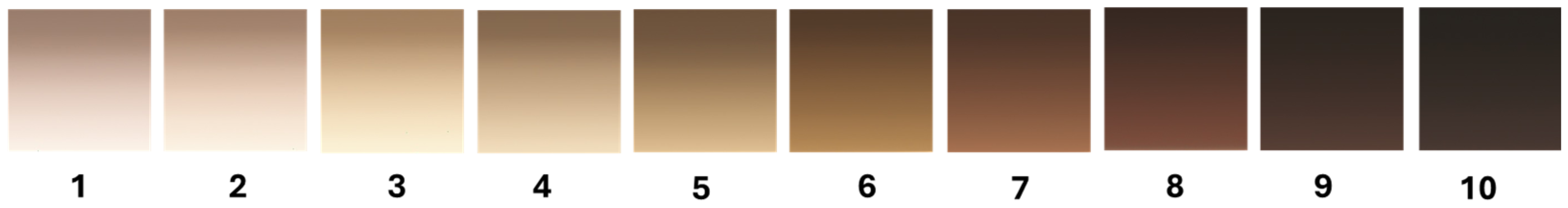
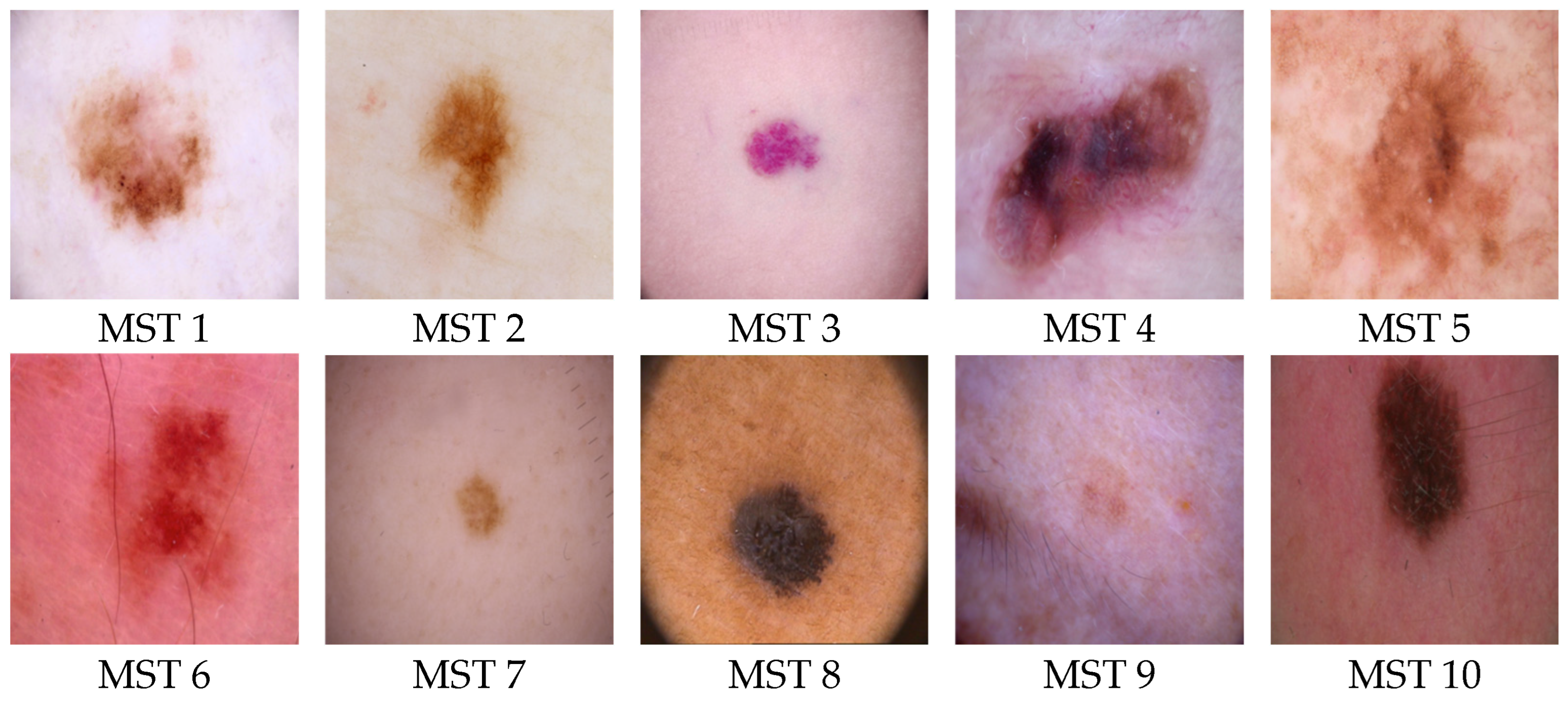
2.2. Skin Color Scales
2.3. Skin Color Estimator
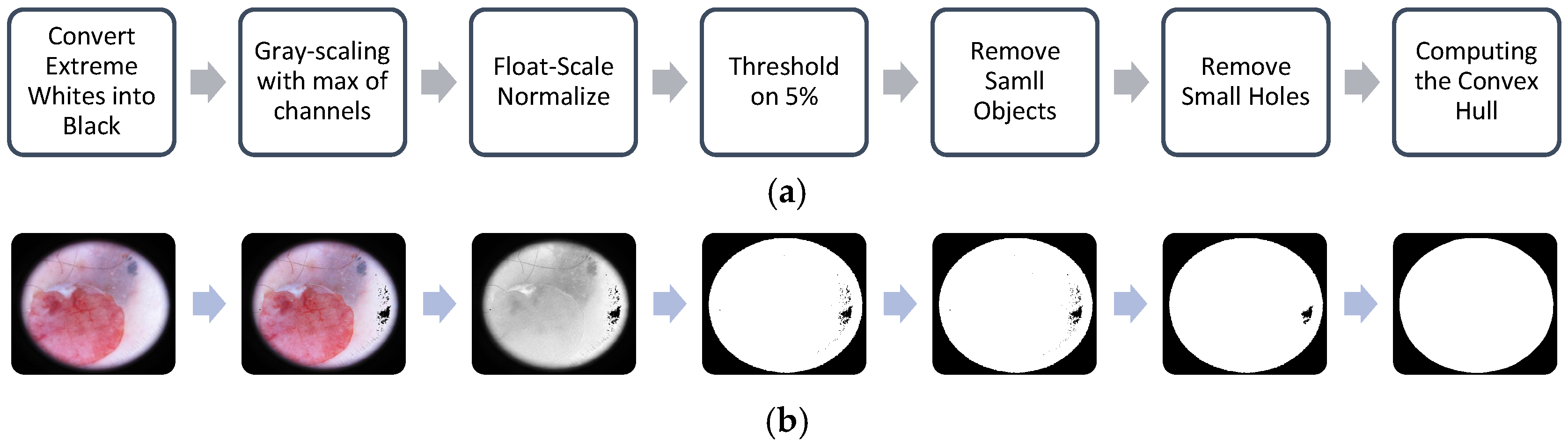
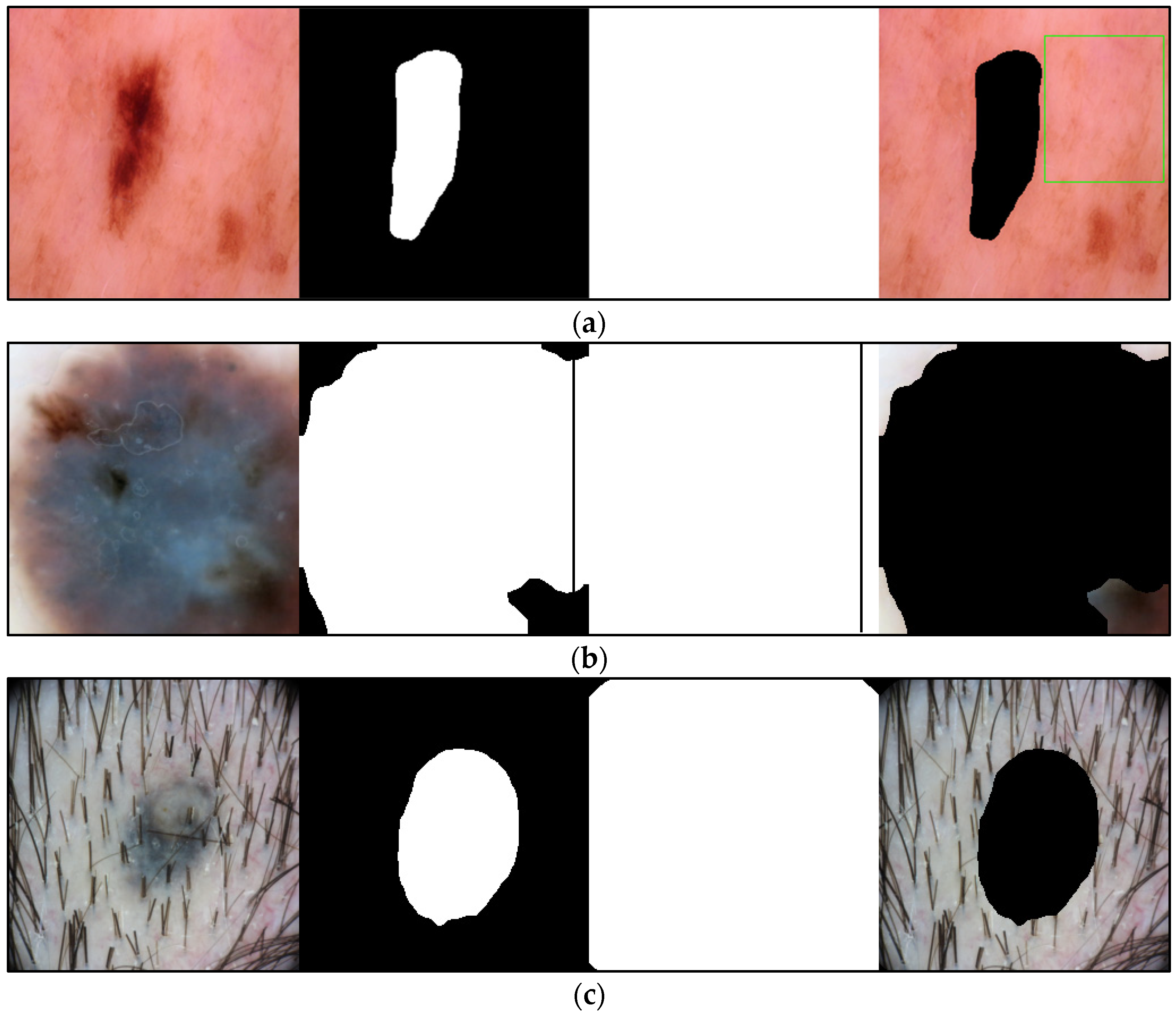
2.3.1. Frame Detection and Removal
| Algorithm 1: Frame segmentation and removal. |
Input
|
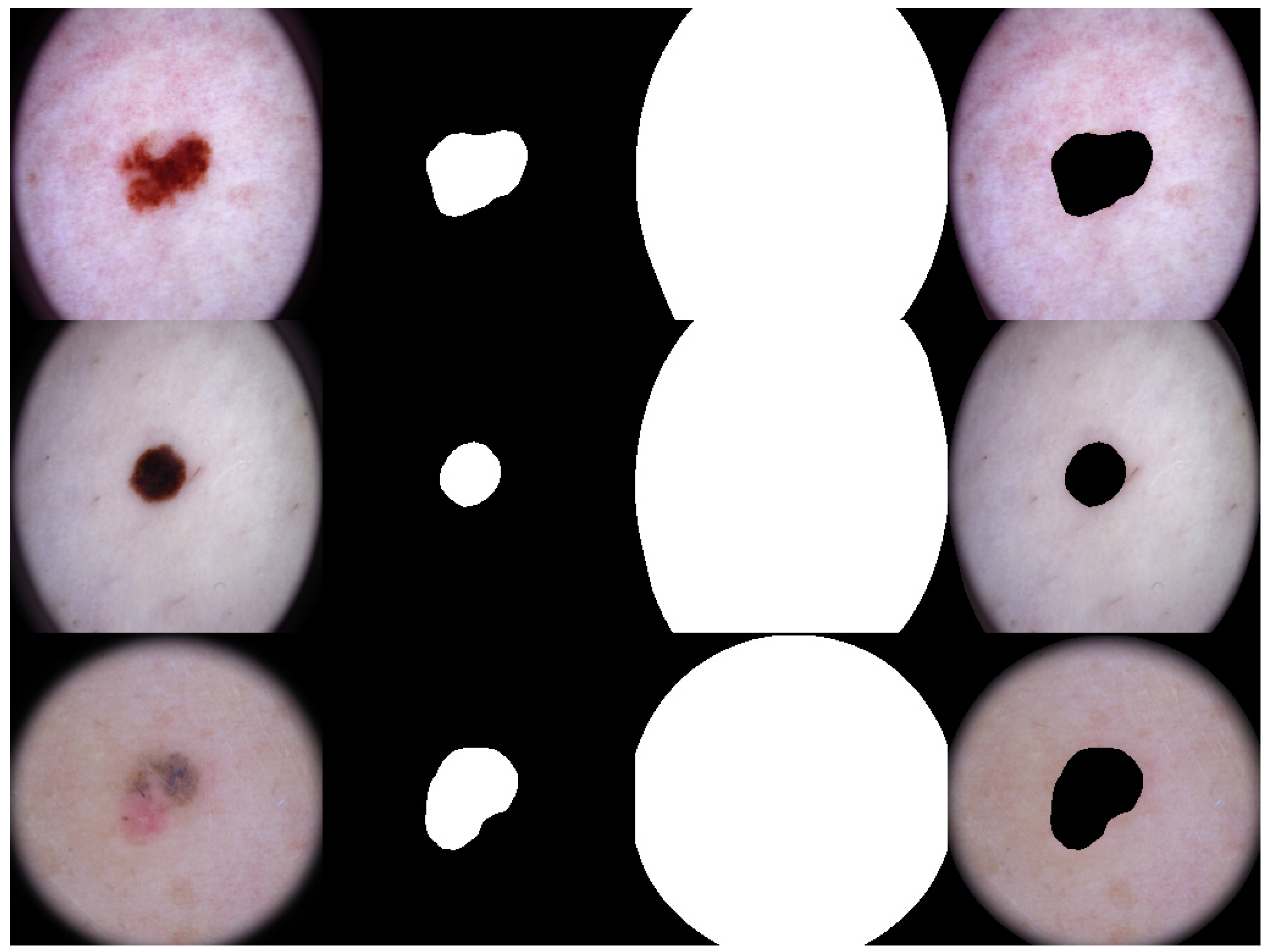
2.3.2. Lesion Segmentation
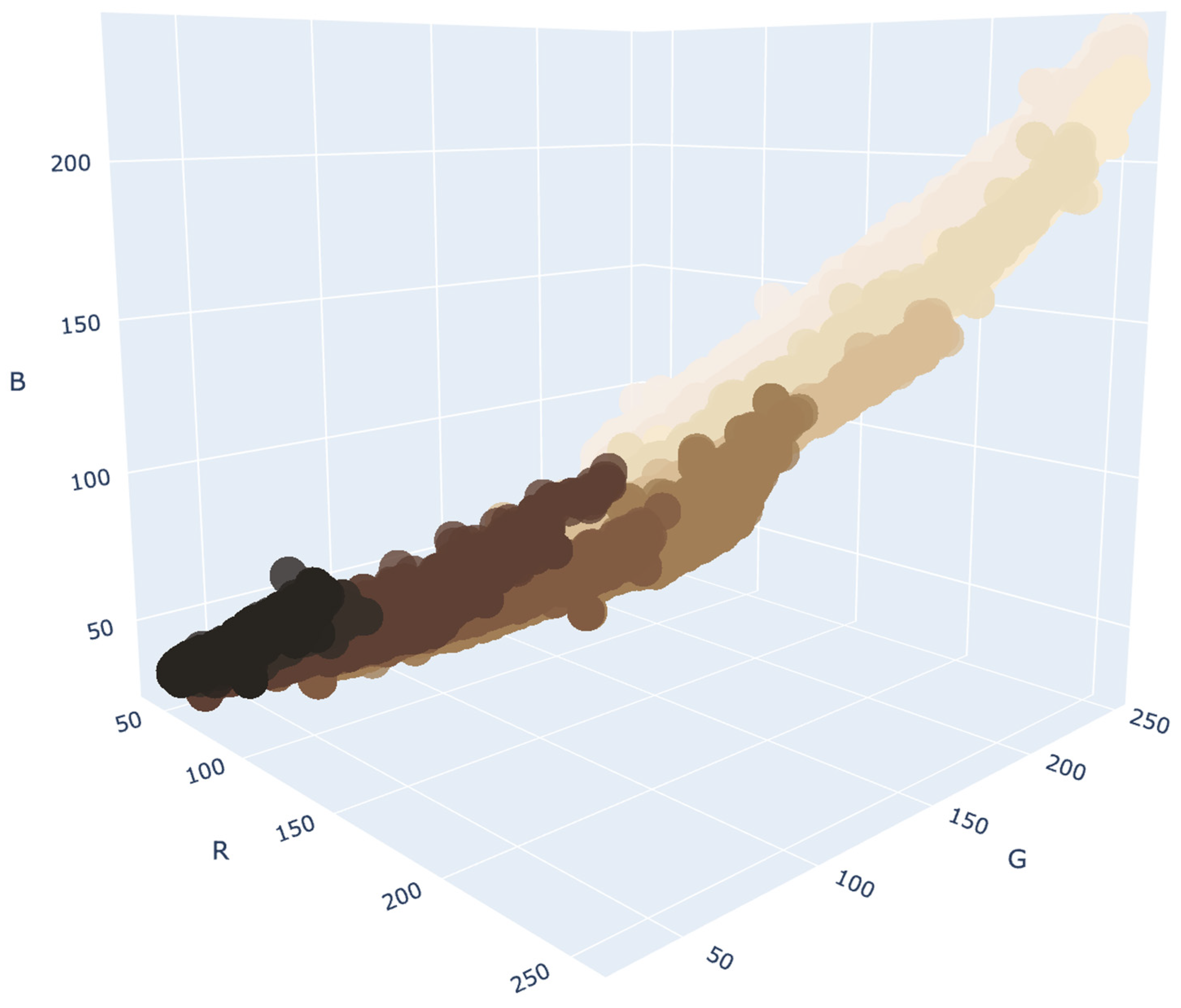
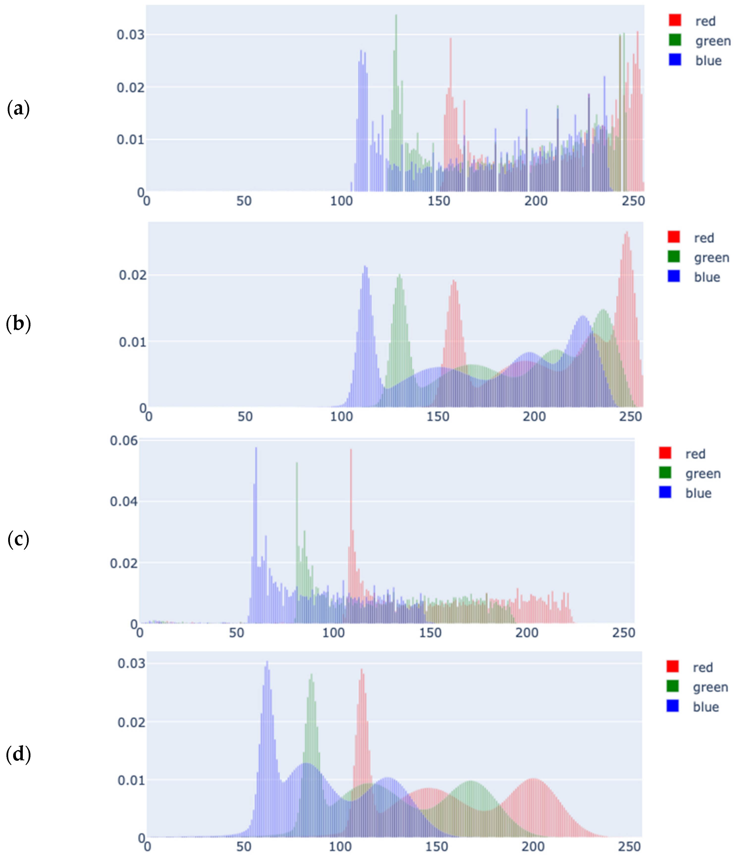
2.3.3. Color Density Estimation
2.3.4. Kullback-Leibler Divergence and Membership Scores
2.4. Test Cohort Annotation
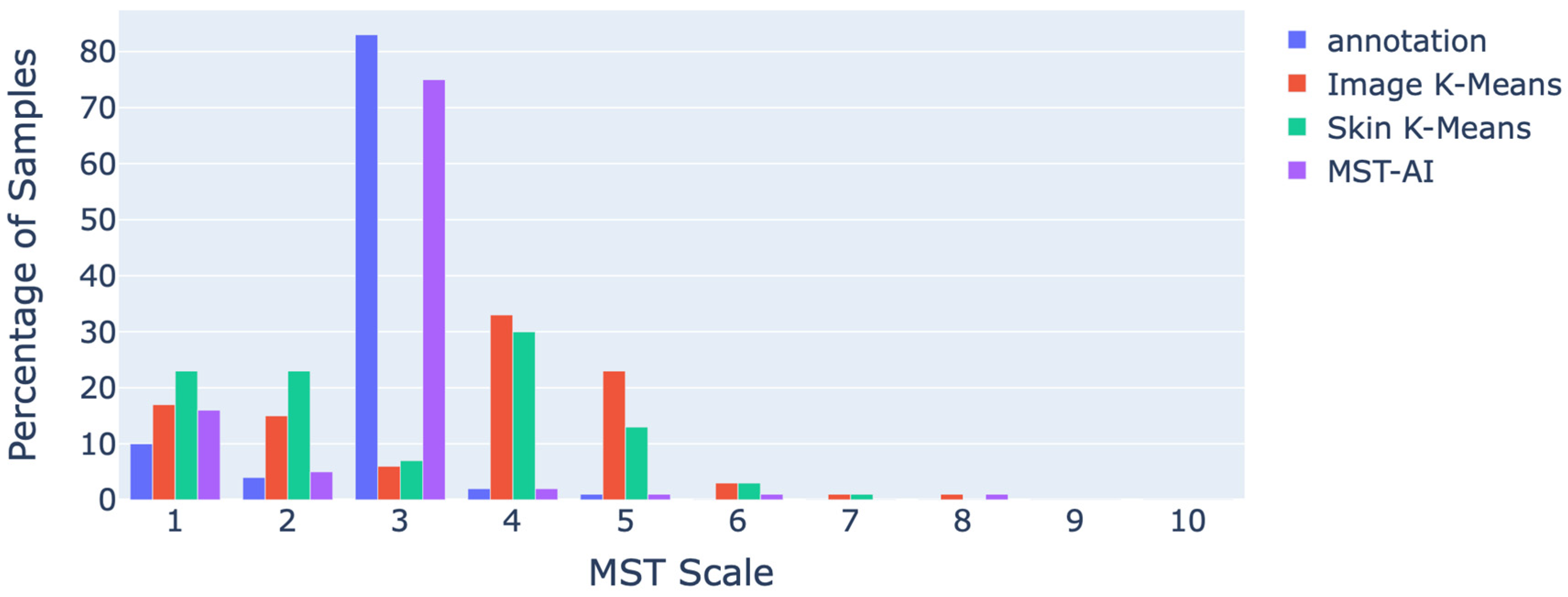
3. Results
4. Discussion
4.1. Statistical Analysis of the Results
4.2. Caveats and Limitations
5. Conclusions
Author Contributions
Funding
Institutional Review Board Statement
Informed Consent Statement
Data Availability Statement
Acknowledgments
Conflicts of Interest
Abbreviations
| AI | Artificial Intelligence |
| ISIC | International Skin Imaging Collaboration |
| MST | Monk Skin Tone |
| GMM | Gaussian Mixture Model |
| VB-GMM | Variational Bayesian Gaussian Mixture Model |
| KLD | Kullback-Leibler Divergence |
| DDI | Stanford Diverse Dermatology Images |
| FST | Fitzpatrick Skin Types |
| ROI | Region of Interest |
| Probability Distribution Function | |
| RGB | Red, Green, Blue |
| NDCG | Normalized Discounted Cumulative Gain |
Appendix A
References
- Guy, G.P.; Thomas, C.C.; Thompson, T.; Watson, M.; Massetti, G.M.; Richardson, L.C.; Centers for Disease Control and Prevention (CDC). Vital Signs: Melanoma Incidence and Mortality Trends and Projections—United States, 1982–2030. MMWR Morb Mortal Wkly. Rep. 2015, 64, 591–596. [Google Scholar] [PubMed]
- Guy, G.P.; Machlin, S.R.; Ekwueme, D.U.; Yabroff, K.R. Prevalence and Costs of Skin Cancer Treatment in the U.S., 2002−2006 and 2007−2011. Am. J. Prev. Med. 2015, 48, 183–187. [Google Scholar] [CrossRef] [PubMed]
- Stern, R.S. Prevalence of a History of Skin Cancer in 2007: Results of an Incidence-Based Model. Arch Dermatol 2010, 146, 279–282. [Google Scholar] [CrossRef]
- American Cancer Society. Cancer Facts & Figures 2025; American Cancer Society: Atlanta, GA, USA, 2025. [Google Scholar]
- Osman, A.; Nigro, A.R.; Brauer, S.F.; Borda, L.J.; Roberts, A.A. Epidemiology and Primary Location of Melanoma in Asian Patients: A Surveillance, Epidemiology, and End Result–Based Study. JAAD Int. 2024, 16, 77–78. [Google Scholar] [CrossRef]
- Townsend, J.S.; Melkonian, S.C.; Jim, M.A.; Holman, D.M.; Buffalo, M.; Julian, A.K. Melanoma Incidence Rates Among Non-Hispanic American Indian/Alaska Native Individuals, 1999–2019. JAMA Dermatol. 2024, 160, 148. [Google Scholar] [CrossRef]
- Mahendraraj, K.; Sidhu, K.; Lau, C.S.M.; McRoy, G.J.; Chamberlain, R.S.; Smith, F.O. Malignant Melanoma in African–Americans: A Population-Based Clinical Outcomes Study Involving 1106 African–American Patients from the Surveillance, Epidemiology, and End Result (SEER) Database (1988–2011). Medicine 2017, 96, e6258. [Google Scholar] [CrossRef]
- Hu, S.; Soza-Vento, R.M.; Parker, D.F.; Kirsner, R.S. Comparison of Stage at Diagnosis of Melanoma Among Hispanic, Black, and White Patients in Miami-Dade County, Florida. Arch. Dermatol. 2006, 142, 704–708. [Google Scholar] [CrossRef]
- Qian, Y.; Johannet, P.; Sawyers, A.; Yu, J.; Osman, I.; Zhong, J. The Ongoing Racial Disparities in Melanoma: An Analysis of the Surveillance, Epidemiology, and End Results Database (1975–2016). J. Am. Acad. Dermatol. 2021, 84, 1585–1593. [Google Scholar] [CrossRef]
- Gregory, C. Mitro Skin Cancer Does Not Discriminate by Skin Tone. 2025. Available online: https://treatcancer.com/blog/skin-cancer-by-skin-tone/ (accessed on 27 May 2025).
- Gupta, A.K.; Bharadwaj, M.; Mehrotra, R. Skin Cancer Concerns in People of Color: Risk Factors and Prevention. Asian Pac. J. Cancer Prev. 2016, 17, 5257. [Google Scholar]
- Zheng, Y.J.; Ho, C.; Lazar, A.; Ortiz-Urda, S. Poor Melanoma Outcomes and Survival in Asian American and Pacific Islander Patients. J. Am. Acad. Dermatol. 2021, 84, 1725–1727. [Google Scholar] [CrossRef]
- Dawes, S.M.; Tsai, S.; Gittleman, H.; Barnholtz-Sloan, J.S.; Bordeaux, J.S. Racial Disparities in Melanoma Survival. J. Am. Acad. Dermatol. 2016, 75, 983–991. [Google Scholar] [CrossRef] [PubMed]
- Gloster, H.M.; Neal, K. Skin Cancer in Skin of Color. J. Am. Acad. Dermatol. 2006, 55, 741–760. [Google Scholar] [CrossRef] [PubMed]
- Huang, H.-Y.; Hsiao, Y.-P.; Mukundan, A.; Tsao, Y.-M.; Chang, W.-Y.; Wang, H.-C. Classification of Skin Cancer Using Novel Hyperspectral Imaging Engineering via YOLOv5. JCM 2023, 12, 1134. [Google Scholar] [CrossRef] [PubMed]
- Redmon, J.; Divvala, S.; Girshick, R.; Farhadi, A. You Only Look Once: Unified, Real-Time Object Detection. In Proceedings of the 2016 IEEE Conference on Computer Vision and Pattern Recognition (CVPR), Las Vegas, NV, USA, 27–30 June 2016; pp. 779–788. [Google Scholar]
- Lin, T.-L.; Lu, C.-T.; Karmakar, R.; Nampalley, K.; Mukundan, A.; Hsiao, Y.-P.; Hsieh, S.-C.; Wang, H.-C. Assessing the Efficacy of the Spectrum-Aided Vision Enhancer (SAVE) to Detect Acral Lentiginous Melanoma, Melanoma In Situ, Nodular Melanoma, and Superficial Spreading Melanoma. Diagnostics 2024, 14, 1672. [Google Scholar] [CrossRef]
- Lin, T.-L.; Karmakar, R.; Mukundan, A.; Chaudhari, S.; Hsiao, Y.-P.; Hsieh, S.-C.; Wang, H.-C. Assessing the Efficacy of the Spectrum-Aided Vision Enhancer (SAVE) to Detect Acral Lentiginous Melanoma, Melanoma In Situ, Nodular Melanoma, and Superficial Spreading Melanoma: Part II. Diagnostics 2025, 15, 714. [Google Scholar] [CrossRef]
- Stephanie, W. Medical Student Melanoma Detection Rates in White and African American Skin Using Moulage and Standardized Patients. CRDOA 2015, 2, 1–4. [Google Scholar] [CrossRef]
- Daneshjou, R.; Smith, M.P.; Sun, M.D.; Rotemberg, V.; Zou, J. Lack of Transparency and Potential Bias in Artificial Intelligence Data Sets and Algorithms: A Scoping Review. JAMA Dermatol. 2021, 157, 1362. [Google Scholar] [CrossRef]
- Tschandl, P. Risk of Bias and Error From Data Sets Used for Dermatologic Artificial Intelligence. JAMA Dermatol. 2021, 157, 1271. [Google Scholar] [CrossRef]
- Daneshjou, R.; Vodrahalli, K.; Novoa, R.A.; Jenkins, M.; Liang, W.; Rotemberg, V.; Ko, J.; Swetter, S.M.; Bailey, E.E.; Gevaert, O.; et al. Disparities in Dermatology AI Performance on a Diverse, Curated Clinical Image Set. Sci. Adv. 2022, 8, eabq6147. [Google Scholar] [CrossRef]
- Fitzpatrick, T.B. The Validity and Practicality of Sun-Reactive Skin Types I Through VI. Arch. Dermatol. 1988, 124, 869. [Google Scholar] [CrossRef]
- Coleman, W.; Mariwalla, K.; Grimes, P. Updating the Fitzpatrick Classification: The Skin Color and Ethnicity Scale. Dermatol. Surg. 2023, 49, 725–731. [Google Scholar] [CrossRef]
- Hazirbas, C.; Bitton, J.; Dolhansky, B.; Pan, J.; Gordo, A.; Ferrer, C.C. Casual Conversations: A Dataset for Measuring Fairness in AI. In Proceedings of the 2021 IEEE/CVF Conference on Computer Vision and Pattern Recognition Workshops (CVPRW), Nashville, TN, USA, 19–25 June 2021; pp. 2289–2293. [Google Scholar]
- Howard, J.J.; Sirotin, Y.B.; Tipton, J.L.; Vemury, A.R. Reliability and Validity of Image-Based and Self-Reported Skin Phenotype Metrics. IEEE Trans. Biom. Behav. Identity Sci. 2021, 3, 550–560. [Google Scholar] [CrossRef]
- Heldreth, C.M.; Monk, E.P.; Clark, A.T.; Schumann, C.; Eyee, X.; Ricco, S. Which Skin Tone Measures Are the Most Inclusive? An Investigation of Skin Tone Measures for Artificial Intelligence. ACM J. Responsib. Comput. 2024, 1, 1–21. [Google Scholar] [CrossRef]
- Bevan, P.J.; Atapour-Abarghouei, A. Detecting Melanoma Fairly: Skin Tone Detection and Debiasing for Skin Lesion Classification. In MICCAI Workshop on Domain Adaptation and Representation Transfer; Springer Nature: Cham, Switzerland, 2022. [Google Scholar]
- Caffery, L.J.; Clunie, D.; Curiel-Lewandrowski, C.; Malvehy, J.; Soyer, H.P.; Halpern, A.C. Transforming Dermatologic Imaging for the Digital Era: Metadata and Standards. J. Digit. Imaging 2018, 31, 568–577. [Google Scholar] [CrossRef]
- Codella, N.; Rotemberg, V.; Tschandl, P.; Celebi, M.E.; Dusza, S.; Gutman, D.; Helba, B.; Kalloo, A.; Liopyris, K.; Marchetti, M.; et al. Skin Lesion Analysis Toward Melanoma Detection 2018: A Challenge Hosted by the International Skin Imaging Collaboration (ISIC). arXiv 2019, arXiv:1902.03368. [Google Scholar]
- Gutman, D.; Codella, N.C.F.; Celebi, E.; Helba, B.; Marchetti, M.; Mishra, N.; Halpern, A. Skin Lesion Analysis toward Melanoma Detection: A Challenge at the International Symposium on Biomedical Imaging (ISBI) 2016, Hosted by the International Skin Imaging Collaboration (ISIC). arXiv 2016, arXiv:1605.01397. [Google Scholar]
- Codella, N.C.F.; Gutman, D.; Celebi, M.E.; Helba, B.; Marchetti, M.A.; Dusza, S.W.; Kalloo, A.; Liopyris, K.; Mishra, N.; Kittler, H.; et al. Skin Lesion Analysis toward Melanoma Detection: A Challenge at the 2017 International Symposium on Biomedical Imaging (ISBI), Hosted by the International Skin Imaging Collaboration (ISIC). In Proceedings of the 2018 IEEE 15th International Symposium on Biomedical Imaging (ISBI 2018), Washington, DC, USA, 4–7 April 2018; pp. 168–172. [Google Scholar]
- Monk, E. The Monk Skin Tone Scale. SocArXiv 2023. [Google Scholar] [CrossRef]
- Monk, E. Monk Skin Tone Scale. 2025. Available online: https://skintone.google (accessed on 27 May 2025).
- Barber, C.B.; Dobkin, D.P.; Huhdanpaa, H. The Quickhull Algorithm for Convex Hulls. ACM Trans. Math. Softw. 1996, 22, 469–483. [Google Scholar] [CrossRef]
- Long, J.; Shelhamer, E.; Darrell, T. Fully Convolutional Networks for Semantic Segmentation. arXiv 2014, arXiv:1411.4038. [Google Scholar] [CrossRef]
- Paszke, A.; Gross, S.; Massa, F.; Lerer, A.; Bradbury, J.; Chanan, G.; Killeen, T.; Lin, Z.; Gimelshein, N.; Antiga, L.; et al. PyTorch: An Imperative Style, High-Performance Deep Learning Library. arXiv 2019, arXiv:1912.01703. [Google Scholar]
- Schölkopf, B.; Smola, A.J. Learning with Kernels: Support Vector Machines, Regularization, Optimization, and Beyond; Adaptive computation and machine learning series; Reprint; MIT Press: Cambridge, MA, USA, 2002; ISBN 978-0-262-53657-8. [Google Scholar]
- Kendall, M.G. A New Measure of Rank Correlation. Biometrika 1938, 30, 81. [Google Scholar] [CrossRef]
- Kendall, M.G. THE TREATMENT OF TIES IN RANKING PROBLEMS. Biometrika 1945, 33, 239–251. [Google Scholar] [CrossRef]
- Kokoska, S.; Zwillinger, D. CRC Standard Probability and Statistics Tables and Formulae, Student Edition; CRC Press: Boca Raton, FL, USA, 2000; ISBN 978-0-429-18146-7. [Google Scholar]


| Year | Train | Malignant% | Valid | Malignant% | Test | Malignant% | Total | Malignant% |
|---|---|---|---|---|---|---|---|---|
| 2016 | 900 | 19.22 | 0 | 0.00 | 379 | 19.79 | 1279 | 19.39 |
| 2017 | 2000 | 18.70 | 150 | 20.00 | 600 | 19.50 | 2750 | 18.95 |
| 2018 | 10,015 | 19.51 | 193 | 22.80 | 1512 | 20.30 | 11,720 | 19.67 |
| 2019 | 25,331 | 36.87 | 0 | 0.00 | N/A | N/A | 25,331 | 36.87 |
| 2020 | 33,126 | 1.76 | 0 | 0.00 | N/A | N/A | 33,126 | 1.76 |
| Year | Train | Valid | Test | Total |
|---|---|---|---|---|
| 2016 | 900/900 | 0 | 379/379 | 1279/1279 |
| 2017 | 2000/2000 | 150/150 | 600/600 | 2750/2750 |
| 2018 | 2594/10,015 | 100/193 | 1000/1512 | 3694/11,720 |
| 2019 | 0 | 0 | 0 | 0 |
| 2020 | 0 | 0 | 0 | 0 |
| Train | Validation | Test | |
|---|---|---|---|
| Jaccard Loss | 0.0046 | 0.0071 | 0.0075 |
| DICE | 94.07% | 89.50% | 89.39% |
| Original Image | 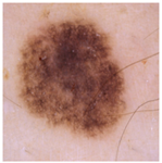 | 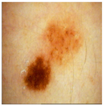 | 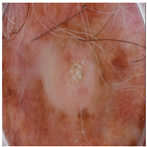 |
| Annotated Region | 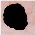 | 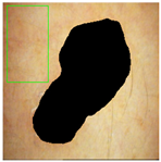 | 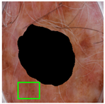 |
| Image K-Means MST scale Memberships |  5,4,6,7 0.151, 0.128, 0.113, 0.101 |  4,5,3,1 0.143, 0.137, 0.114, 0.108 |  6,7,5,8 0.152, 0.138, 0.128, 0.113 |
| Skin K-Means MST scale Memberships |  2,1,3,4 0.140, 0.138, 0.136, 0.120 |  3,2,1,4 0.140, 0.140, 0.136, 0.124 |  5,4,6,3 0.145, 0.128, 0.114, 0.102 |
| MST-AI MST scale Memberships |  1,2,3,4 0.133, 0.129, 0.118, 0.117 |  5,3,4,6 0.130, 0.127, 0.125, 0.121 |  8,1,2,7 0.149, 0.139, 0.120, 0.117 |
| Metric | Image K-Means | Skin K-Means | MST-AI | |||||||||
|---|---|---|---|---|---|---|---|---|---|---|---|---|
| @1 | @2 | @3 | @4 | @1 | @2 | @3 | @4 | @1 | @2 | @3 | @4 | |
| Kendall’s Tau | - | 0.12 | 0.12 | −0.02 | - | 0.12 | 0.17 | −0.05 | - | 0.78 | 0.73 | 0.74 |
| Spearman’s Correlation | - | 0.12 | 0.13 | −0.06 | - | 0.12 | 0.18 | −0.10 | - | 0.78 | 0.73 | 0.74 |
| NDCG | 0.89 | 0.90 | 0.91 | 0.92 | 0.91 | 0.93 | 0.94 | 0.94 | 0.99 | 0.99 | 0.99 | 1.00 |
| Top-k | Correlations | NDCG |
|---|---|---|
| top-1 | N/A |  |
| top-2 |  |  |
| top-3 |  |  |
| top-4 |  |  |
Disclaimer/Publisher’s Note: The statements, opinions and data contained in all publications are solely those of the individual author(s) and contributor(s) and not of MDPI and/or the editor(s). MDPI and/or the editor(s) disclaim responsibility for any injury to people or property resulting from any ideas, methods, instructions or products referred to in the content. |
© 2025 by the authors. Licensee MDPI, Basel, Switzerland. This article is an open access article distributed under the terms and conditions of the Creative Commons Attribution (CC BY) license (https://creativecommons.org/licenses/by/4.0/).
Share and Cite
Khalkhali, V.; Lee, H.; Nguyen, J.; Zamora-Erazo, S.; Ragin, C.; Aphale, A.; Bellacosa, A.; Monk, E.P.; Biswas, S.K. MST-AI: Skin Color Estimation in Skin Cancer Datasets. J. Imaging 2025, 11, 235. https://doi.org/10.3390/jimaging11070235
Khalkhali V, Lee H, Nguyen J, Zamora-Erazo S, Ragin C, Aphale A, Bellacosa A, Monk EP, Biswas SK. MST-AI: Skin Color Estimation in Skin Cancer Datasets. Journal of Imaging. 2025; 11(7):235. https://doi.org/10.3390/jimaging11070235
Chicago/Turabian StyleKhalkhali, Vahid, Hayan Lee, Joseph Nguyen, Sergio Zamora-Erazo, Camille Ragin, Abhishek Aphale, Alfonso Bellacosa, Ellis P. Monk, and Saroj K. Biswas. 2025. "MST-AI: Skin Color Estimation in Skin Cancer Datasets" Journal of Imaging 11, no. 7: 235. https://doi.org/10.3390/jimaging11070235
APA StyleKhalkhali, V., Lee, H., Nguyen, J., Zamora-Erazo, S., Ragin, C., Aphale, A., Bellacosa, A., Monk, E. P., & Biswas, S. K. (2025). MST-AI: Skin Color Estimation in Skin Cancer Datasets. Journal of Imaging, 11(7), 235. https://doi.org/10.3390/jimaging11070235