
AI-Driven Automated Blood Cell Anomaly Detection: Enhancing Diagnostics and Telehealth in Hematology


Abstract
1. Introduction
1.1. Context
1.2. Challenges
1.3. Key Contributions
- Development of a unified pipeline that combines segmentation, classification, transfer learning, and zero-shot learning (ZSL) techniques.
- Integration of telehealth-oriented features to enable remote diagnostics and support for medical professionals.
- Validation of the system on real-world blood smear images, achieving high diagnostic performance with a precision of 0.98, recall of 0.99, and an F1 score of 0.98.
1.4. Paper Organization
2. Background
2.1. Hematology Overview
2.1.1. Blood Components
- Plasma (55%)—the liquid portion of blood.
- Blood Cells (45%)—which includes red blood cells (RBCs), white blood cells (WBCs)—as shown in Figure 1—and platelets.
- Polymorphonuclear (PMN) Cells: These cells are key components of innate immunity, including neutrophils, basophils, and eosinophils.
- Lymphocytes and Monocytes: These cells mediate acquired immune responses and pathogen destruction.
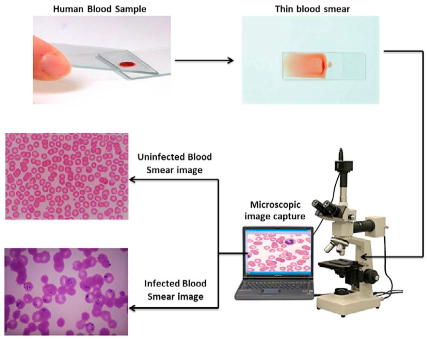
2.1.2. Blood Tests and Smear Imaging
- Evaluate organ function (e.g., kidneys, liver, heart).
- Diagnose infections, anemia, and chronic conditions.
- Monitor disease progression or treatment effectiveness.
- Complete blood count (CBC).
- Blood chemistry and enzyme analysis.
- Risk markers for cardiovascular diseases.
- A drop of blood is spread thinly on a glass slide.
- The slide is examined under an optical microscope.
- A digital camera captures high-resolution images of blood cells.
- The images are saved and analyzed for abnormalities (see Figure 2).
2.2. Machine Learning Techniques
2.2.1. Segmentation Models
2.2.2. Classification Models
2.2.3. Transfer Learning
2.2.4. Zero-Shot Learning (ZSL)
2.2.5. Geometry Learning
2.2.6. Transformer Models
3. Related Work
3.1. Related Works
- Hegde et al. (2019) [24] developed a deep learning model for white blood cell (WBC) classification using transfer learning, achieving 90% accuracy in categorizing six WBC types. Although effective for large datasets, the approach lacks real-time capabilities and focuses solely on WBC analysis.
- Kutlu et al. (2020) [25] proposed a CNN-based system achieving 94.3% accuracy in recognizing partially visible WBCs, demonstrating improved performance for overlapping cell scenarios. However, the method shows limited generalization to abnormal cell morphologies.
- Akalin et al. (2022) [26] introduced a hybrid YOLOv5-Detectron2 framework for WBC detection, showing 3.44–14.7% accuracy improvements over individual models. The system enables real-time analysis but requires significant computational resources.
- Rahman et al. (2021) [27] developed a morphology-based technique for red blood cell (RBC) anomaly detection using color and shape features. Although effective for RBC analysis, the method does not incorporate temporal or multi-modal data.
- Gill et al. (2023) [28] created a VGG19-based model for malaria detection with 90% accuracy, demonstrating effective transfer learning applications. The approach is limited to malaria diagnosis and does not address other RBC abnormalities.
- Pasupa et al. (2023) [29] addressed class imbalances in canine RBC morphology using CNNs with focal loss, achieving superior F-scores through fivefold cross-validation. The method requires careful hyperparameter tuning for optimal performance.
- Khan et al. (2024) [30] developed an RCNN-based model that achieved 99% training and 91.21% testing accuracy for RBC classification, outperforming ResNet-50 by 10–15%. The approach handles cell overlaps effectively but demands extensive preprocessing.
- Onakpojeruo et al. (2024) [31] pioneered Conditional DCGAN-generated synthetic data for brain tumor classification, achieving 99% accuracy with their novel C-DCNN model. Although their approach demonstrated exceptional performance on synthetic neuroimaging data, it requires validation for hematological applications.
- Onakpojeruo et al. (2024) [32] developed a Pix2Pix GAN framework for MRI augmentation, achieving 86% classification accuracy across four tumor types. Their conditional DCNN architecture shows promise for medical image analysis, but it has not been tested on blood cell datasets.
3.2. Novelty of the Proposed System
- Real-Time Processing: Unlike existing systems with high computational demands, real-time analysis is enabled through optimized models like YOLOv11, achieving an inference latency of 50 ms per image, suitable for telehealth settings [26].
- Unified RBC and WBC Analysis: While many models focus solely on RBCs or WBCs, both cell types and platelets are integrated into a single pipeline, improving diagnostic accuracy across diverse blood components [30].
- Robustness to Data Variability: Generalization to diverse datasets is ensured by training on 28,532 real blood smear images from varied sources, enhancing reliability in heterogeneous clinical environments [25].
- Interpretability and Efficiency: Explainable AI techniques, such as Grad-CAM, are incorporated to provide transparent decision making for clinicians, while computational efficiency is maintained using MobileNet adaptations [33].
- Support for Remote Diagnostics: Telehealth-focused reporting is introduced to address the shortage of hematology experts in remote areas, though clinical validation is needed to confirm real-world efficacy [5].
4. Proposed Approach
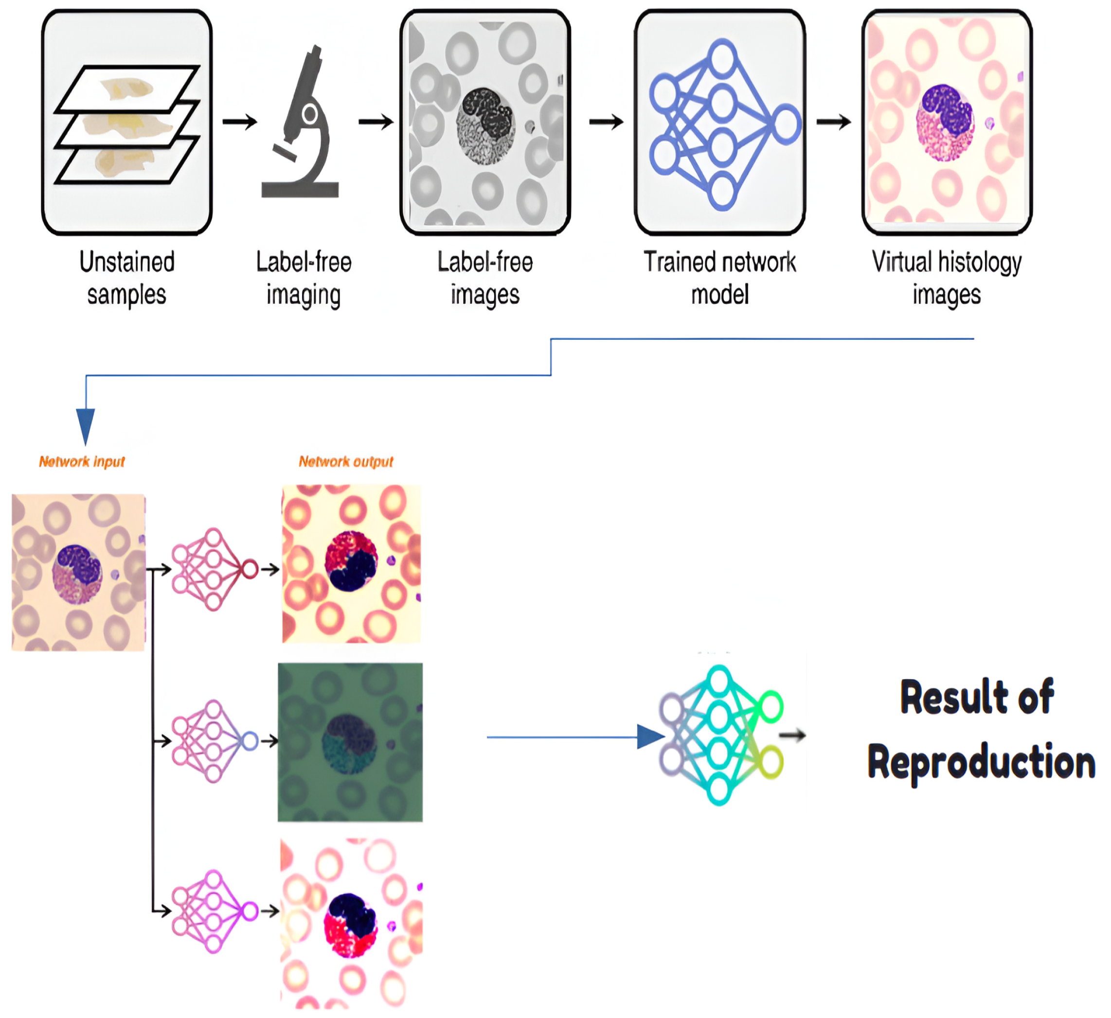
4.1. Step 0: Virtual Histological Staining Using Deep Learning
4.1.1. Development of a Virtual Staining Model
4.1.2. Training and Inference of Transformation Networks
4.1.3. Network Architecture and Training Strategies
4.2. Step 1: Segmentation and Detection Model
4.3. Step 2: Classification Model
4.4. Step 3-1: Correction Model Using Zero-Shot Learning
4.5. Step 3-2: Feature Extraction Using Transfer Learning
4.6. Step 4: Anomaly Detection Using Geometric Learning
4.7. Step 5: Report Generation Using Machine Learning Methods
5. Experimentation and Validation
5.1. Used Datasets
5.1.1. Primary Dataset Description
- Histology slides prepared for electron microscopy;
- Human blood samples collected through clinical procedures;
- Curated images from established online medical repositories.
- Basophil, eosinophil, lymphocyte, monocyte, myelocyte, and neutrophil;
- Erythroblast and red blood cell (RBC);
- Intrusion (imaging artifacts) and platelet.
5.1.2. Public Benchmark Dataset: ALL-IDB
- ALL-IDB1: A total of 108 images containing 390 annotated cells for segmentation tasks
- ALL-IDB2: A total of 260 images with balanced healthy/leukemic samples for classification.
5.1.3. Data Preparation Pipeline
- Duplicate elimination: Removed 142 redundant samples using perceptual hashing.
- Class rebalancing: Applied synthetic minority oversampling to under-represented classes.
- Annotation standardization: Converted all labels to YOLO-compatible text format, where each image is associated with a .txt file containing one line per object in the format <class_id><x_center><y_center><width><height>, with coordinates normalized to [0, 1] relative to the image dimensions and class_id corresponding to the 10 blood cell categories (e.g., 0 for basophil, 1 for eosinophil, etc.).
- Geometric augmentation: Generated variations through flips (horizontal/vertical), rotations (), and shear transformations (0.2 rad).
- Pixel normalization: Scaled intensities to the [0, 1] range per channel.
5.2. Experimental Protocol
- Fivefold Stratified Cross-Validation:
- –
- Fixed random seed (42) for reproducible splits.
- –
- Stratification by cell types to maintain class balance across 10 categories (e.g., basophil, eosinophil, etc.).
- –
- A 80:20 train/validation ratio per fold (e.g., 6704 training and 1676 validation images per fold for the private dataset pre-augmentation; 22,826 training and 5706 validation images post-augmentation).
- L2 Regularization ():
- –
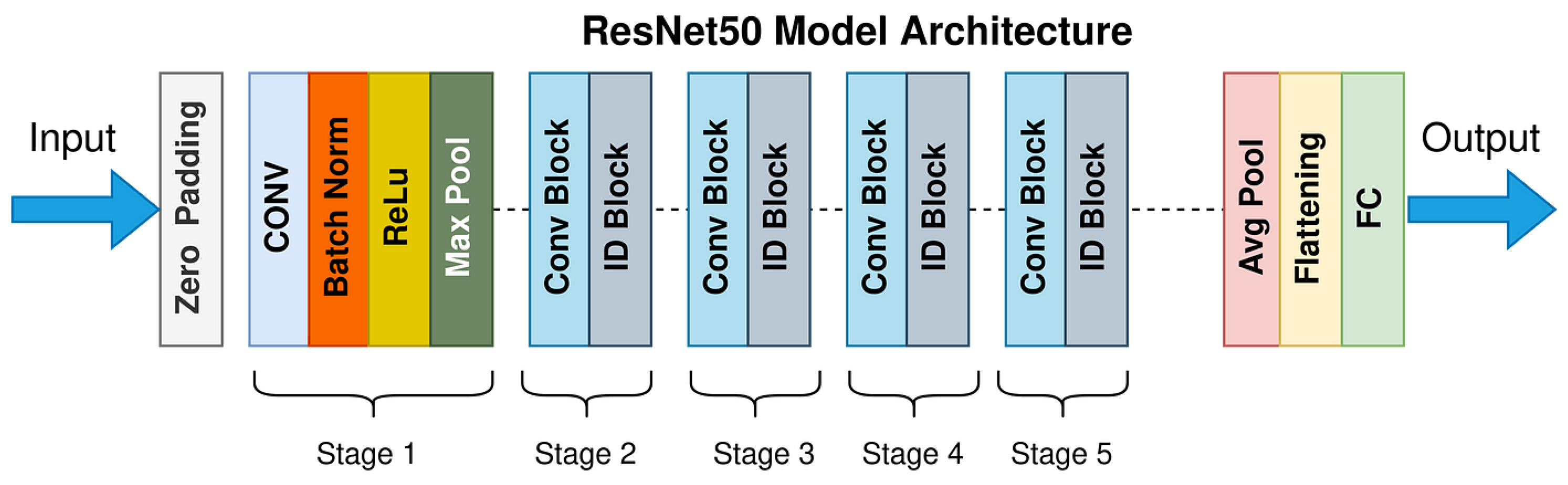
- Applied to both CNN and Transformer components (e.g., in YOLO and ResNet50 models).
- –
- Penalty strength tuned via grid search on validation folds.
- –
- Normalized by feature counts to ensure consistency across. models.
- Held-out Test Set:
- –
- A total of 1100 images (private dataset) and 20% of ALL-IDB (e.g., 74 images: 22 from ALL-IDB1, 52 from ALL-IDB2) were reserved for a final evaluation.
- –
- Balanced across cell types (10 classes for the private dataset, 2 classes for ALL-IDB).
- –
- Never used during training or hyperparameter tuning.
- Statistical Testing:
- –
- Paired t-tests () on fold-wise metrics (accuracy, F1 score).
- –
- Bonferroni correction for multiple comparisons.
- –
- Effect sizes reported via Cohen’s d.
5.3. Model Evaluation
5.3.1. Threshold Optimization
5.3.2. Segmentation and Detection Model
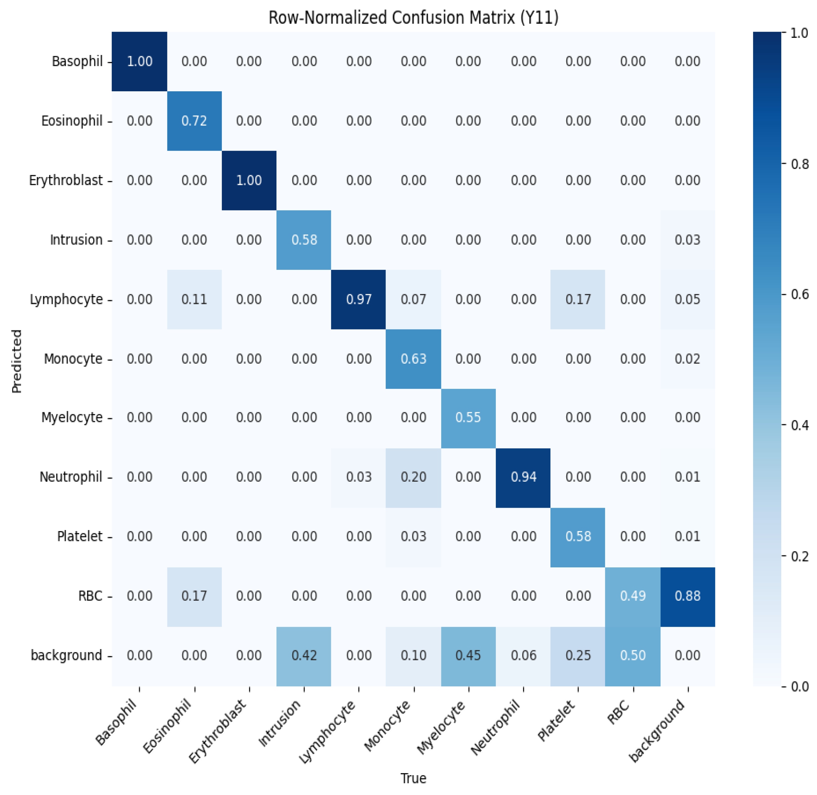
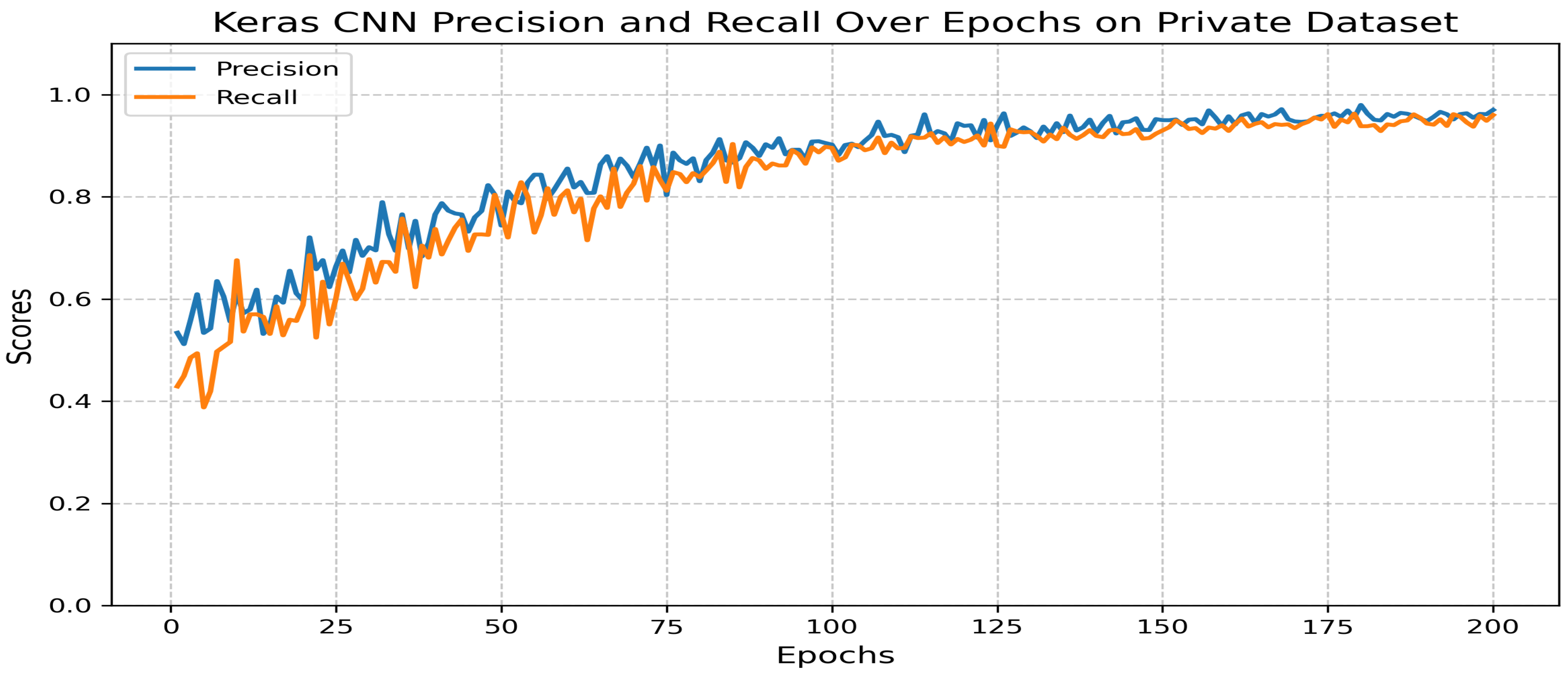
5.3.3. Classification Model
- Precision: 0.97.
- Recall: 0.96.
- F1 score: 0.97.
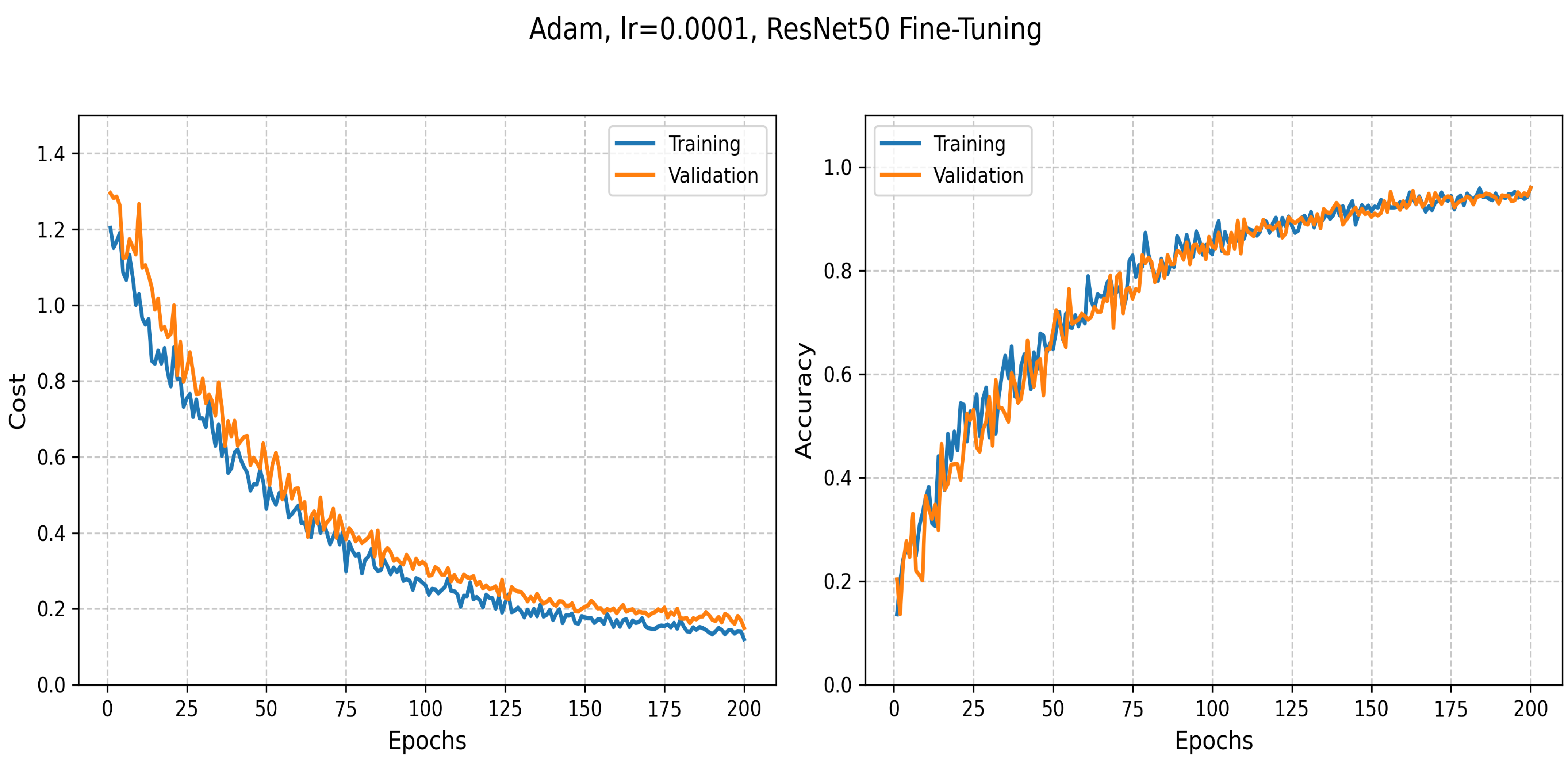
5.3.4. Transfer Learning: ResNet50-Based Classification
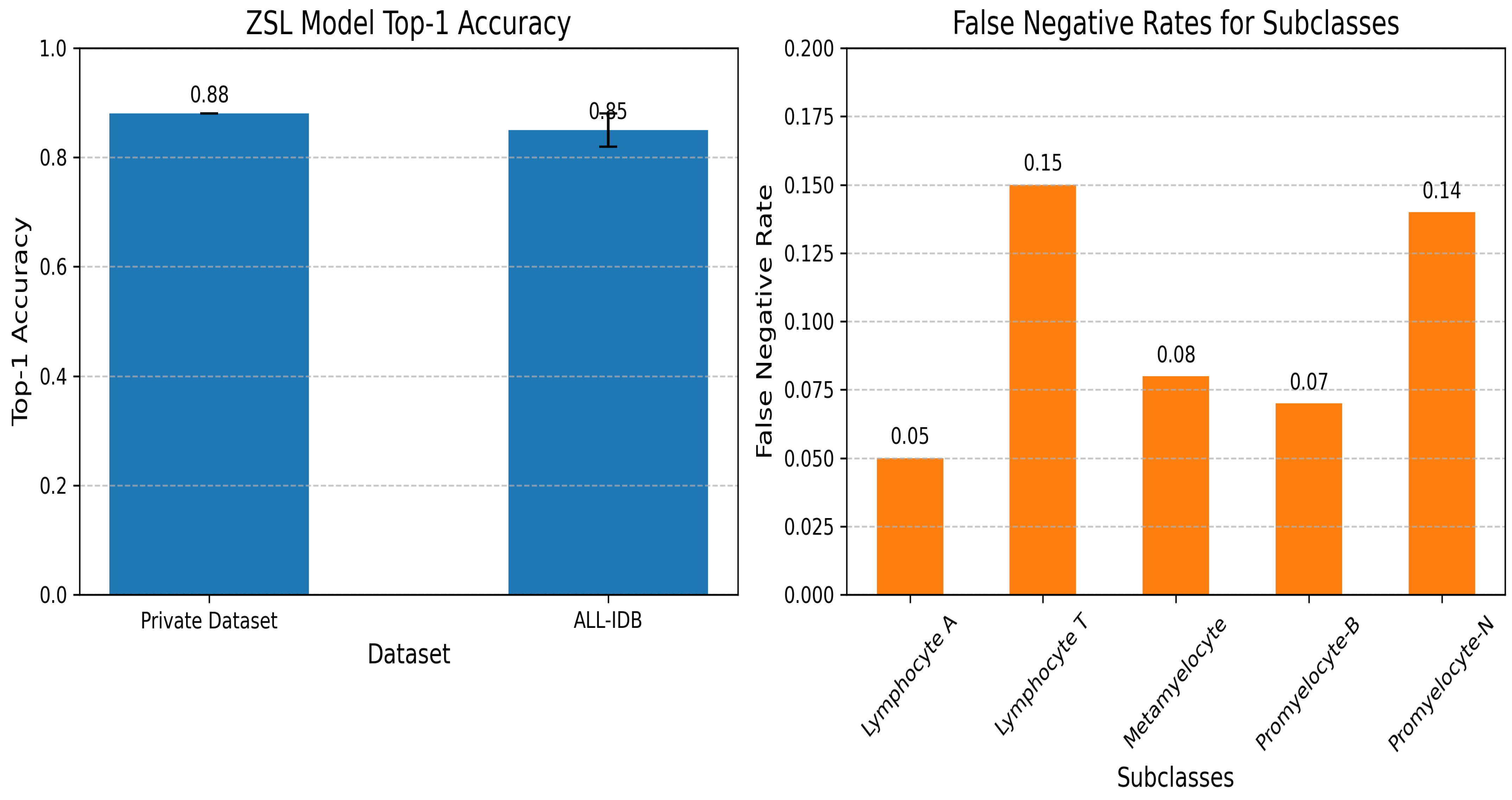
5.3.5. Zero-Shot Learning Model for Subclass Creation
5.3.6. Geometry Learning Model
5.3.7. Machine Learning-Based Classification and Preprocessing Techniques
- Outlier Detection:
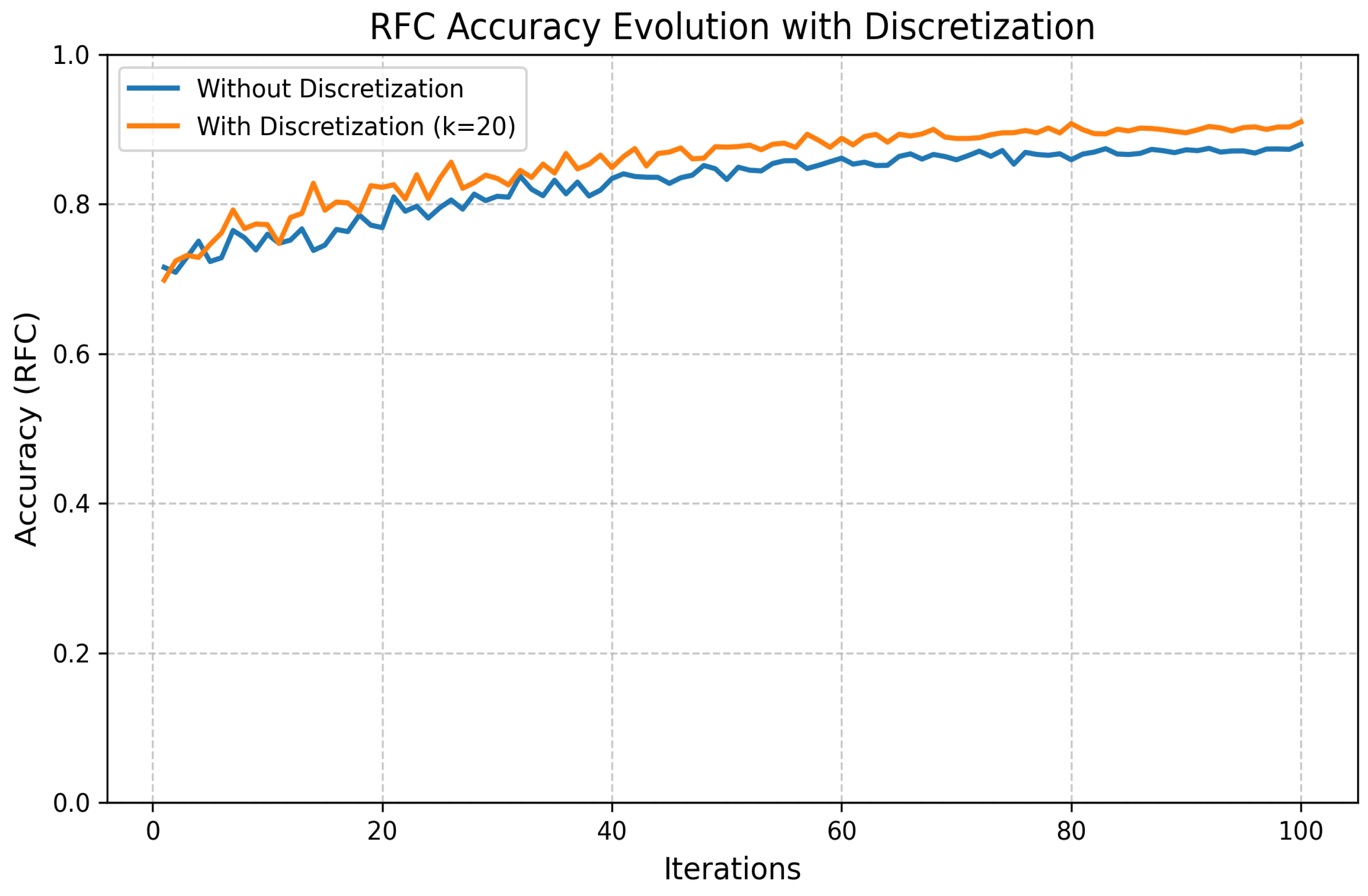
- Discretization:
5.4. Statistical Validation
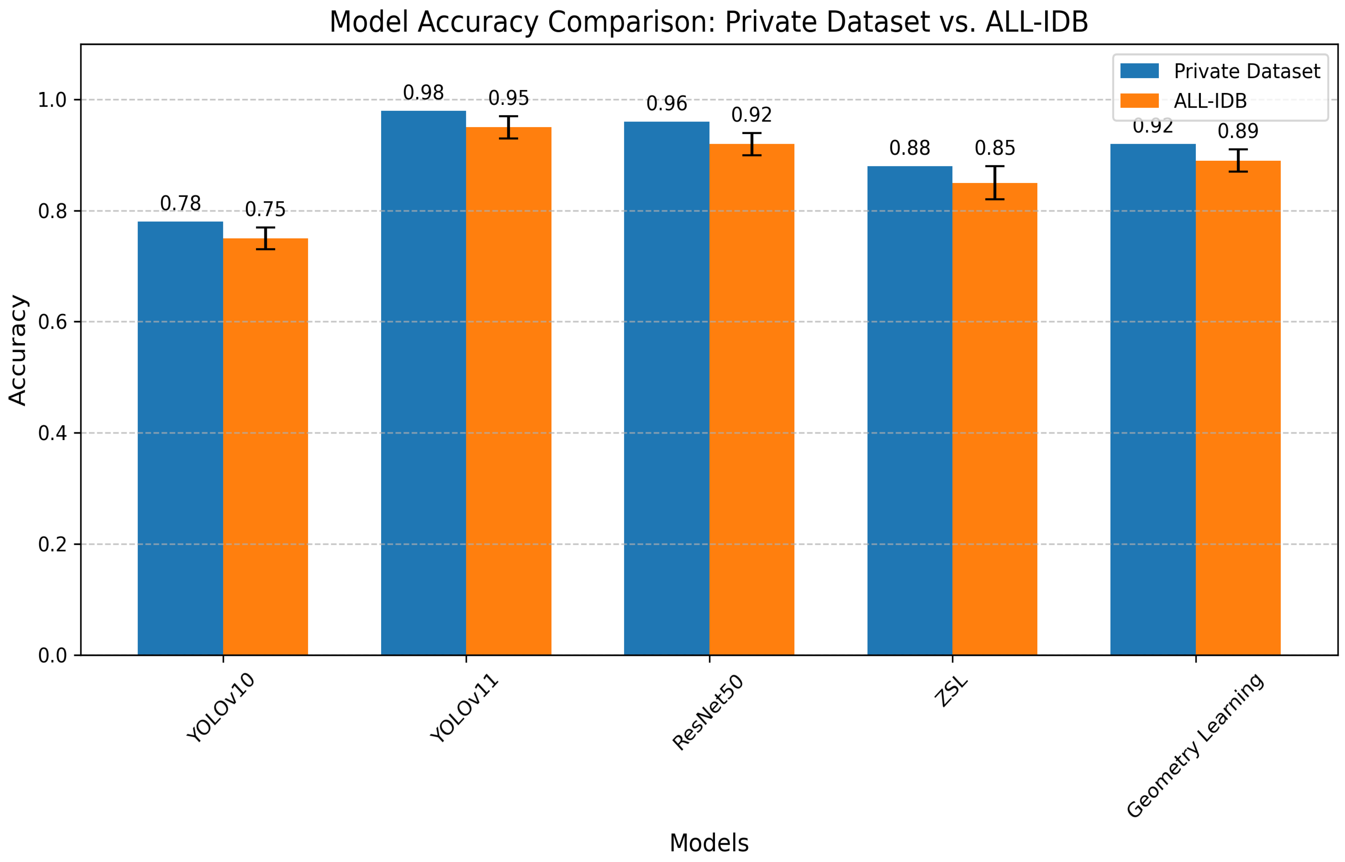
5.5. Results’ Comparison
5.5.1. Segmentation and Detection Performance
- YOLOv11 outperforms all comparative models in precision (98%) and F1 score (0.98).
- Our approach maintains advantages in both detection accuracy (surpassing [25] by 3.7%) and computational efficiency.
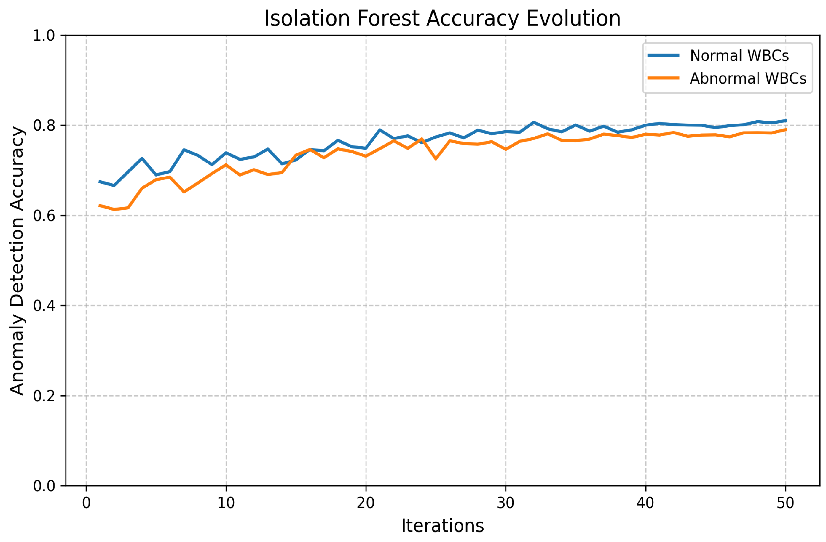
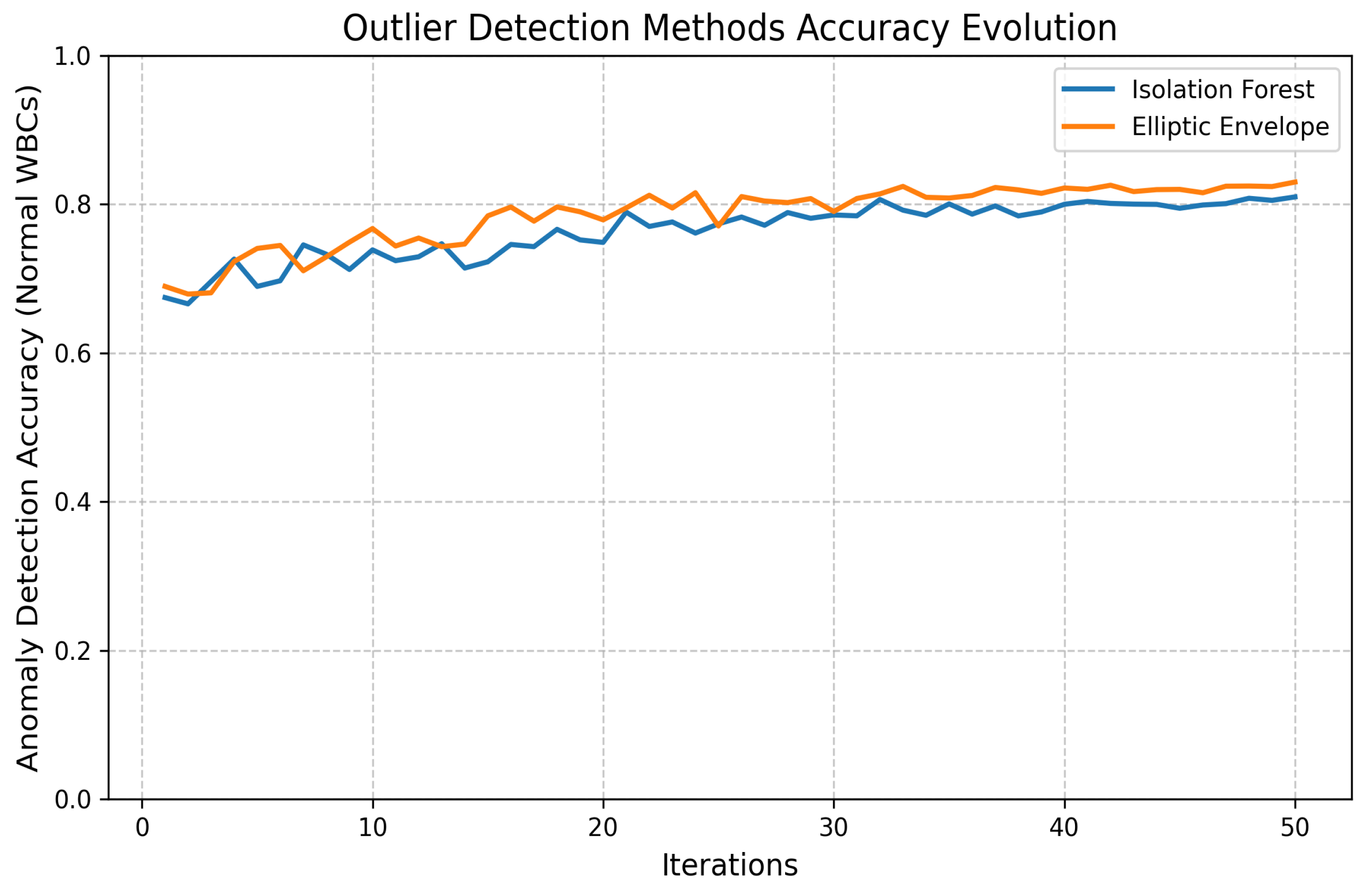
5.5.2. Machine Learning Methods’ Performance
- Automatic Outlier Detection Method:

| Model | Model Precision | F1 Score | Decision Time |
|---|---|---|---|
| RandomForestClassifier | 0.977778 | 0.977778 | 0.002229 |
| DecisionTreeClassifier | 0.952778 | 0.937778 | 0.039439 |
| GradientBoostingClassifier | 0.930006 | 0.915556 | 0.047807 |
- Elliptic Envelope Method:
| Model | Model Precision | F1 Score | Decision Time |
|---|---|---|---|
| AdaBoostClassifier | 1.000000 | 1.000000 | 0.035010 |
| GradientBoostingClassifier | 0.977778 | 0.971429 | 0.041291 |
| DecisionTreeClassifier | 0.977778 | 0.971429 | 0.049943 |
- Discretization Method:
| Model | Model Precision | F1 Score | Decision Time |
|---|---|---|---|
| GradientBoostingClassifier | 0.952778 | 0.904762 | 0.037799 |
| RandomForestClassifier | 0.952778 | 0.904762 | 0.049618 |
| MLPClassifier | 0.952778 | 0.904762 | 0.086684 |
6. Discussion
7. Conclusions and Future Work
- A unified pipeline addressing segmentation, classification, and novel anomaly detection.
- Implementation of explainable AI techniques for clinical interpretability.
- Optimization for rapid inference (50 ms/image) without sacrificing accuracy.
- Clinical validation: Pending trials comparing system performance against board-certified hematologists across diverse healthcare settings.
- Data diversity: Expansion of training corpora to include (a) broader demographic representation and (b) standardized ethical documentation.
Author Contributions
Funding
Institutional Review Board Statement
Informed Consent Statement
Data Availability Statement
Conflicts of Interest
References
- Blann, A.; Ahmed, N. Blood Science: Principles and Pathology; John Wiley & Sons: Hoboken, NJ, USA, 2022. [Google Scholar]
- Padalko, E.; Colenbie, L.; Delforge, A.; Ectors, N.; Guns, J.; Imbert, R.; Jansens, H.; Pirnay, J.-P.; Rodenbach, M.-P.; Van Riet, I.; et al. Preanalytical variables influencing the interpretation and reporting of biological tests on blood samples of living and deceased donors for human body materials. Cell Tissue Bank. 2024, 25, 509–520. [Google Scholar] [CrossRef] [PubMed]
- Walter, W.; Haferlach, C.; Nadarajah, N.; Schmidts, I.; Kühn, C.; Kern, W.; Haferlach, T. How artificial intelligence might disrupt diagnostics in hematology in the near future. Oncogene 2021, 40, 4271–4280. [Google Scholar] [CrossRef] [PubMed]
- Obstfeld, A.E. Hematology and machine learning. J. Appl. Lab. Med. 2023, 8, 129–144. [Google Scholar] [CrossRef] [PubMed]
- Anilkumar, K.K.; Manoj, V.J.; Sagi, T.M. A survey on image segmentation of blood and bone marrow smear images with emphasis to automated detection of Leukemia. Biocybern. Biomed. Eng. 2020, 40, 1406–1420. [Google Scholar] [CrossRef]
- Allgaier, J.; Mulansky, L.; Draelos, R.L.; Pryss, R. How does the model make predictions? A systematic literature review on the explainability power of machine learning in healthcare. Artif. Intell. Med. 2023, 143, 102616. [Google Scholar] [CrossRef]
- Chhabra, G. Automated hematology analyzers: Recent trends and applications. J. Lab. Physicians 2018, 10, 15–16. [Google Scholar] [CrossRef]
- Malgoyre, A.; Bigard, X.; Alonso, A.; Sanchez, H.; Kelberine, F. Variabilité des compositions cellulaire et moléculaire des extraits de concentrés plaquettaires (platelet-rich plasma, PRP). J. Traumatol. Sport 2012, 29, 236–240. [Google Scholar] [CrossRef]
- Xu, Y.; Quan, R.; Xu, W.; Huang, Y.; Chen, X.; Liu, F. Advances in Medical Image Segmentation: A Comprehensive Review of Traditional, Deep Learning and Hybrid Approaches. Bioengineering 2024, 11, 1034. [Google Scholar] [CrossRef]
- Misra, V.; Mall, A.K. Harnessing Image Processing for Precision Disease Diagnosis in Sugar Beet Agriculture. Crop Des. 2024, 3, 100075. [Google Scholar] [CrossRef]
- Terven, J.; Córdova-Esparza, D.-M.; Romero-González, J.-A. A comprehensive review of yolo architectures in computer vision: From yolov1 to yolov8 and yolo-nas. Mach. Learn. Knowl. Extr. 2023, 5, 1680–1716. [Google Scholar] [CrossRef]
- Grandini, M.; Bagli, E.; Visani, G. Metrics for multi-class classification: An overview. arXiv 2020, arXiv:2008.05756. [Google Scholar]
- Asif, S.; Ti, W.; Ur-Rehman, S.; Ul-Ain, Q.; Amjad, K.; Yi, Y.; Si, J.; Awais, M. Advancements and Prospects of Machine Learning in Medical Diagnostics: Unveiling the Future of Diagnostic Precision. In Archives of Computational Methods in Engineering; Springer: Berlin/Heidelberg, Germany, 2024; pp. 1–31. [Google Scholar]
- Mukherjee, S. The Annotated ResNet-50: Explaining How ResNet-50 Works and Why It Is So Popular. 2022. Available online: https://towardsdatascience.com/the-annotated-resnet-50-a6c536034758/ (accessed on 20 March 2025).
- Simonyan, K.; Zisserman, A. Very deep convolutional networks for large-scale image recognition. arXiv 2014, arXiv:1409.1556. [Google Scholar]
- He, K.; Zhang, X.; Ren, S.; Sun, J. Deep residual learning for image recognition. In Proceedings of the IEEE Conference on Computer Vision and Pattern Recognition, Las Vegas, NV, USA, 27–30 June 2016. [Google Scholar]
- Sandler, M.; Howard, A.; Zhu, M.; Zhmoginov, A.; Chen, L.C. Mobilenetv2: Inverted residuals and linear bottlenecks. In Proceedings of the IEEE Conference on Computer Vision and Pattern Recognition, Salt Lake City, UT, USA, 18–22 June 2018. [Google Scholar]
- Cao, W.; Wu, Y.; Sun, Y.; Zhang, H.; Ren, J.; Gu, D.; Wang, X. A review on multimodal zero-shot learning. Wiley Interdiscip. Rev. Data Min. Knowl. Discov. 2023, 13, e1488. [Google Scholar] [CrossRef]
- Guo, J.; Rao, Z.; Chen, Z.; Zhou, J.; Tao, D. Fine-grained zero-shot learning: Advances, challenges, and prospects. arXiv 2024, arXiv:2401.17766. [Google Scholar]
- Liu, Z.; Zhang, X.; Zhu, Z.; Zheng, S.; Zhao, Y.; Cheng, J. MFHI: Taking modality-free human identification as zero-shot learning. IEEE Trans. Circuits Syst. Video Technol. 2021, 32, 5225–5237. [Google Scholar] [CrossRef]
- Meng, Y.; Zhang, Y.; Xie, J.; Duan, J.; Joddrell, M.; Madhusudhan, S.; Peto, T.; Zhao, Y.; Zheng, Y. Multi-granularity learning of explicit geometric constraint and contrast for label-efficient medical image segmentation and differentiable clinical function assessment. Med. Image Anal. 2024, 95, 103183. [Google Scholar] [CrossRef]
- Vijayalakshmi, A. Deep learning approach to detect malaria from microscopic images. Multimed. Tools Appl. 2020, 79, 15297–15317. [Google Scholar] [CrossRef]
- Yang, F.; Wang, X.; Ma, H.; Li, J. Transformers-sklearn: A toolkit for medical language understanding with transformer-based models. BMC Med. Inform. Decis. Mak. 2021, 21, 90. [Google Scholar] [CrossRef]
- Hegde, R.B.; Prasad, K.; Hebbar, H.; Singh, B.M.K. Comparison of traditional image processing and deep learning approaches for classification of white blood cells in peripheral blood smear images. Biocybern. Biomed. Eng. 2019, 39, 382–392. [Google Scholar] [CrossRef]
- Kutlu, H.; Avci, E.; Özyurt, F. White blood cells detection and classification based on regional convolutional neural networks. Med. Hypotheses 2020, 135, 109472. [Google Scholar] [CrossRef]
- Akalin, F.; Yumuşak, N. Detection and classification of white blood cells with an improved deep learning-based approach. Turk. J. Electr. Eng. Comput. Sci. 2022, 30, 2725–2739. [Google Scholar] [CrossRef]
- Rahman, S.; Azam, B.; Khan, S.U.; Awais, M.; Ali, I. Automatic identification of abnormal blood smear images using color and morphology variation of RBCS and central pallor. Comput. Med Imaging Graph. 2021, 87, 101813. [Google Scholar] [CrossRef] [PubMed]
- Gill, K.S.; Anand, V.; Gupta, R. An Efficient VGG19 Framework for Malaria Detection in Blood Cell Images. In Proceedings of the IEEE 2023 3rd Asian Conference on Innovation in Technology (ASIANCON), Pune, India, 25–27 August 2023. [Google Scholar]
- Pasupa, K.; Vatathanavaro, S.; Tungjitnob, S. Convolutional neural networks based focal loss for class imbalance problem: A case study of canine red blood cells morphology classification. J. Ambient Intell. Humaniz. Comput. 2023, 14, 15259–15275. [Google Scholar] [CrossRef]
- Khan, R.U.; Almakdi, S.; Alshehri, M.; Haq, A.U.; Ullah, A.; Kumar, R. An intelligent neural network model to detect red blood cells for various blood structure classification in microscopic medical images. Heliyon 2024, 10, 13. [Google Scholar] [CrossRef]
- Onakpojeruo, E.P.; Mustapha, M.T.; Ozsahin, D.U.; Ozsahin, I. A comparative analysis of the novel conditional deep convolutional neural network model, using conditional deep convolutional generative adversarial network-generated synthetic and augmented brain tumor datasets for image classification. Brain Sci. 2024, 14, 559. [Google Scholar] [CrossRef]
- Onakpojeruo, E.P.; Mustapha, M.T.; Ozsahin, D.U.; Ozsahin, I. Enhanced MRI-based brain tumour classification with a novel Pix2pix generative adversarial network augmentation framework. Brain Commun. 2024, 6, fcae372. [Google Scholar] [CrossRef]
- Saarela, M.; Podgorelec, V. Recent applications of Explainable AI (XAI): A systematic literature review. Appl. Sci. 2024, 14, 8884. [Google Scholar] [CrossRef]
- Bai, B.; Yang, X.; Li, Y.; Zhang, Y.; Pillar, N.; Ozcan, A. Deep learning-enabled virtual histological staining of biological samples. Light. Sci. Appl. 2023, 12, 57. [Google Scholar] [CrossRef]
- Udayakumar, D.; Doğan, B.E. Dynamic Contrast-Enhanced MRI. Magnetic Resonance Imaging Clinics of North America. 2024. Available online: https://www.sciencedirect.com/topics/medicine-and-dentistry/dynamic-contrast-enhanced-mri (accessed on 20 March 2025).
- Labati, R.D.; Piuri, V.; Scotti, F. ALL-IDB: The acute lymphoblastic leukemia image database for image processing. In Proceedings of the 2011 18th IEEE International Conference on Image Processing, Brussels, Belgium, 11–14 September 2011; pp. 2045–2048. [Google Scholar]
- Wang, W.; Zheng, V.W.; Yu, H.; Miao, C. A survey of zero-shot learning: Settings, methods, and applications. ACM Trans. Intell. Syst. Technol. (TIST) 2019, 10, 13. [Google Scholar] [CrossRef]
- McEwen, J.D.; Wallis, C.G.R.; Mavor-Parker, A.N. Scattering networks on the sphere for scalable and rotationally equivariant spherical CNNs. arXiv 2021, arXiv:2102.02828. [Google Scholar]
- Rajak, A.; Shrivastava, A.K.; Vidushi. Applying and comparing machine learning classification algorithms for predicting the results of students. J. Discret. Math. Sci. Cryptogr. 2020, 23, 419–427. [Google Scholar] [CrossRef]
- Tanwar, V.; Sharma, B.; Yadav, D.P.; Dwivedi, A.D. Enhancing Blood Cell Diagnosis Using Hybrid Residual and Dual Block Transformer Network. Bioengineering 2025, 12, 98. [Google Scholar] [CrossRef]


| Category | Details |
|---|---|
| Role in Immunity | WBCs are the primary effectors of immunity, acting as protective cells against various forms of aggression. |
| Alternative Name | White blood cells are also known as leukocytes. |
| Classification | WBCs are classified into the following cells:
|
| Origin | All blood cells originate from a single multipotent cell in the bone marrow. |
| Development Process | Maturing cells acquire structural and functional properties during hematopoiesis. |
| Study | Approach | Advantages | Limitations/Interpretability |
|---|---|---|---|
| Hegde et al. (2019) [24] | Transfer learning for WBC classification | 90% accuracy; scalable for large datasets | No real-time analysis; WBC-only focus |
| Kutlu et al. (2020) [25] | CNN for partial WBC recognition | 94.3% accuracy; handles overlapping cells | Limited to normal WBC morphologies |
| Akalin et al. (2022) [26] | YOLOv5-Detectron2 hybrid model | 3.44–14.7% accuracy gain; real-time capable | Computationally intensive |
| Rahman et al. (2021) [27] | Morphological RBC analysis | Effective color/shape-based detection | Single-modality approach |
| Gill et al. (2023) [28] | VGG19 for malaria detection | 90% accuracy; automated diagnosis | Malaria-specific application |
| Pasupa et al. (2023) [29] | CNN with focal loss | Handles class imbalance; high F-scores | Requires hyperparameter optimization |
| Khan et al. (2024) [30] | RCNN for RBC classification | 99% training accuracy; handles cell overlaps | Computationally demanding |
| Onakpojeruo et al. (2024) [31] | Conditional DCGAN + C-DCNN | 99% accuracy; privacy-preserving | Neuroimaging-specific validation |
| Onakpojeruo et al. (2024) [32] | Pix2Pix GAN augmentation | 86% accuracy; multi-class capability | Untested for hematological analysis |
| Segmentation Type | Partition | Images | Classes/Image |
|---|---|---|---|
| Multi-class | Training | 8380 | 2–10 |
| Multi-class | Validation | 2600 | 2–8 |
| Multi-class | Test | 1100 | 1–6 |
| Characteristic | Primary Dataset | ALL-IDB |
|---|---|---|
| Samples | 12,080 (pre-augmentation) | 368 |
| Classes | 10 (cell types) | 2 (normal/leukemic) |
| Demographics | Multi-source | Pediatric focus |
| Annotation Quality | 99.5% complete | 100% complete |
| Task Type | Multi-class segmentation | Binary classification |
| Cell Type | Original Samples | Augmented Samples |
|---|---|---|
| Basophil | 4200 | 7590 |
| Eosinophil | 3032 | 6804 |
| Erythroblast | 2050 | 6390 |
| Intrusion | 1590 | 5200 |
| Lymphocyte | 3620 | 6980 |
| Monocyte | 5307 | 8352 |
| Myelocyte | 4165 | 7490 |
| Neutrophil | 5270 | 8298 |
| Platelet | 4986 | 7916 |
| RBC | 8706 | 10,380 |
| Metric | Original Model | Optimized Model | Improvement |
|---|---|---|---|
| Latency | 0.0199 s/batch | 0.0035 s/batch | 3.13× |
| Throughput | 91.66 data/s | 286.69 data/s | 3.13× |
| Model Size | 44.98 MB | 32.37 MB | −28% |
| Metric Drop | - | 0.0363 | - |
| Metric | YOLOv10 Train | YOLOv10 Val | YOLOv11 Train | YOLOv11 Val |
|---|---|---|---|---|
| Box Loss | 1.0 | 0.9 | 0.8 | 0.7 |
| Segmentation Loss | 1.5 | 1.2 | 1.2 | 1.0 |
| Classification Loss | 0.5 | 0.6 | 0.4 | 0.5 |
| DFL Loss | 0.9 | 1.0 | 0.7 | 0.8 |
| Precision (B) | 0.8 | 0.7 | 0.99 | 0.98 |
| Recall (B) | 0.7 | 0.6 | 0.98 | 0.97 |
| mAP@50 (B) | 0.7 | 0.6 | 0.95 | 0.94 |
| mAP@50:95 (B) | 0.5 | 0.4 | 0.75 | 0.73 |
| Precision (M) | 0.7 | 0.6 | 0.98 | 0.97 |
| Recall (M) | 0.6 | 0.5 | 0.97 | 0.96 |
| mAP@50 (M) | 0.6 | 0.5 | 0.94 | 0.93 |
| mAP@50:95 (M) | 0.4 | 0.3 | 0.72 | 0.70 |
| Hyperparameter | Value |
|---|---|
| Learning Rate | 0.001 |
| Batch Size | 16 |
| Optimizer | Adam |
| Epochs | 200 |
| Momentum | 0.9 |
| Weight Decay | 0.0005 |
| Hyperparameter | Value |
|---|---|
| Learning rate | 0.001 |
| Batch size | 32 |
| Number of epochs | 50 |
| Optimizer | Adam |
| Loss function | Binary Cross-Entropy |
| Activation function | ReLU (hidden layers), Sigmoid (output) |
| Dropout rate | 0.5 |
| Number of convolutional layers | 3 |
| Kernel size | 3 × 3 |
| Pooling type | MaxPooling (2 × 2) |
| Early stopping | Enabled (patience = 5) |
| Hyperparameter | Value |
|---|---|
| Pre-trained weights | ImageNet |
| Learning rate | 0.0001 |
| Batch size | 32 |
| Epochs | 200 |
| Optimizer | Adam |
| Loss function | Categorical Cross-Entropy |
| Activation (dense layers) | ReLU |
| Final activation | Softmax |
| Dropout rate | 0.5 |
| Trainable layers | Top 50% of the model |
| Early stopping | Enabled (patience = 10) |
| Data augmentation | Enabled (rotation, flip, shift) |
| Hyperparameter | Value |
|---|---|
| Learning rate | 0.001 |
| Batch size | 16 |
| Epochs | 100 |
| Optimizer | Adam |
| Loss function | Cross-Entropy |
| Embedding dimension | 300 (GloVe) |
| Dropout rate | 0.3 |
| Regularization | L2 () |
| Early stopping | Enabled (patience = 5) |
| Hyperparameter | Value |
|---|---|
| Learning rate | 0.0005 |
| Batch size | 32 |
| Epochs | 150 |
| Optimizer | Adam |
| Loss function | Mean Squared Error |
| Scattering layers | 3 |
| Wavelet filters | 8 |
| Dropout rate | 0.4 |
| Regularization | L2 () |
| Early stopping | Enabled (patience = 8) |
| Model | Private Dataset | ALL-IDB | Effect Size (d) | Key Advantage | Limitation |
|---|---|---|---|---|---|
| YOLOv11 (Ours) | 0.98 | 0.95 | 1.5 | Real-time processing | Requires GPU acceleration |
| ResNet50 (Ours) | 0.96 | 0.92 | 1.3 | Transfer learning capability | Moderate compute requirements |
| Geometry Learning (Ours) | 0.92 | 0.89 | 1.1 | Shape feature extraction | Specialized for RBC analysis |
| ZSL (Ours) | 0.88 | 0.85 ± 0.03 | 1.0 | Novel subclass detection | Needs semantic embeddings |
| YOLOv10 (Ours) | 0.87 | 0.82 | 0.9 | Balanced speed/accuracy | Lower rare-class recall |
| Onakpojeruo et al. (2024a) [31] | 0.99 * | - | - | Synthetic data generation | Neuroimaging focus |
| Onakpojeruo et al. (2024b) [32] | 0.86 * | - | - | Multi-class augmentation | Untested for hematology |
| ResViT [40] | 0.82 | 0.78 | - | Baseline comparison | Lower accuracy |
| Metric | YOLOv10 | YOLOv11 |
|---|---|---|
| Precision | 0.87 | 0.98 |
| Recall | 0.80 | 0.99 |
| F1 Score | 0.75 | 0.98 |
| Model | Methodology | Precision | F1 Score | Key Advantage |
|---|---|---|---|---|
| YOLOv10 (Ours) | Multi-label segmentation | 87% | 0.75 | Balanced speed/accuracy |
| YOLOv11 (Ours) | Advanced object detection | 98% | 0.98 | State-of-the-art performance |
| Hegde et al. [24] | CNN with transfer learning | 90% | - | WBC classification |
| Kutlu et al. [25] | Partial WBC recognition | 94.3% | - | Handles overlapping cells |
| Akalin et al. [26] | YOLOv5-Detectron2 hybrid | 91.2% * | - | Real-time capability |
| Khan et al. [30] | RCNN with augmentation | 99% ** | - | Touching cell resolution |
Disclaimer/Publisher’s Note: The statements, opinions and data contained in all publications are solely those of the individual author(s) and contributor(s) and not of MDPI and/or the editor(s). MDPI and/or the editor(s) disclaim responsibility for any injury to people or property resulting from any ideas, methods, instructions or products referred to in the content. |
© 2025 by the authors. Licensee MDPI, Basel, Switzerland. This article is an open access article distributed under the terms and conditions of the Creative Commons Attribution (CC BY) license (https://creativecommons.org/licenses/by/4.0/).
Share and Cite
Naouali, S.; El Othmani, O. AI-Driven Automated Blood Cell Anomaly Detection: Enhancing Diagnostics and Telehealth in Hematology. J. Imaging 2025, 11, 157. https://doi.org/10.3390/jimaging11050157
Naouali S, El Othmani O. AI-Driven Automated Blood Cell Anomaly Detection: Enhancing Diagnostics and Telehealth in Hematology. Journal of Imaging. 2025; 11(5):157. https://doi.org/10.3390/jimaging11050157
Chicago/Turabian StyleNaouali, Sami, and Oussama El Othmani. 2025. "AI-Driven Automated Blood Cell Anomaly Detection: Enhancing Diagnostics and Telehealth in Hematology" Journal of Imaging 11, no. 5: 157. https://doi.org/10.3390/jimaging11050157
APA StyleNaouali, S., & El Othmani, O. (2025). AI-Driven Automated Blood Cell Anomaly Detection: Enhancing Diagnostics and Telehealth in Hematology. Journal of Imaging, 11(5), 157. https://doi.org/10.3390/jimaging11050157