Author Contributions
Conceptualization, A.N. and D.N.; methodology, D.S. and D.N.; formal analysis N.O.; software, N.O., V.V. and E.D.; validation, A.N., D.S. and D.N.; investigation, A.N., D.S., N.O., A.S., E.D. and M.Z.; resources, N.O. data curation, N.O., E.D. and M.Z.; writing—original draft preparation, D.S.; writing—review and editing, A.S.; visualization, N.O., V.V., E.D. and M.Z.; supervision, A.N. and D.N.; project administration, D.S.; funding acquisition, A.N. All authors have read and agreed to the published version of the manuscript.
Figure 1.
Examples from RRSHID [
22] showing scenes with significant temporal changes (highlighted with red boxes) between paired hazy and haze-free images.
Figure 1.
Examples from RRSHID [
22] showing scenes with significant temporal changes (highlighted with red boxes) between paired hazy and haze-free images.
Figure 2.
A set of flight-line images consisting of one hazy and one clear image, along with three pairs of manually annotated rectangular areas affected by haze on the hazy flight-line image (highlighted with red boxes).
Figure 2.
A set of flight-line images consisting of one hazy and one clear image, along with three pairs of manually annotated rectangular areas affected by haze on the hazy flight-line image (highlighted with red boxes).
Figure 3.
Pipeline for deriving the RRealHyperPDID dataset from raw AVIRIS flight-line images.
Figure 3.
Pipeline for deriving the RRealHyperPDID dataset from raw AVIRIS flight-line images.
Figure 4.
An example of geometric distortions in AVIRIS data.
Figure 4.
An example of geometric distortions in AVIRIS data.
Figure 5.
Examples of RRealHyperPDID images showing the same area that has changed significantly between acquisitions taken just 19 days apart (18 April 2014 and 7 May 2014).
Figure 5.
Examples of RRealHyperPDID images showing the same area that has changed significantly between acquisitions taken just 19 days apart (18 April 2014 and 7 May 2014).
Figure 6.
Examples of randomly generated maps with parameters .
Figure 6.
Examples of randomly generated maps with parameters .
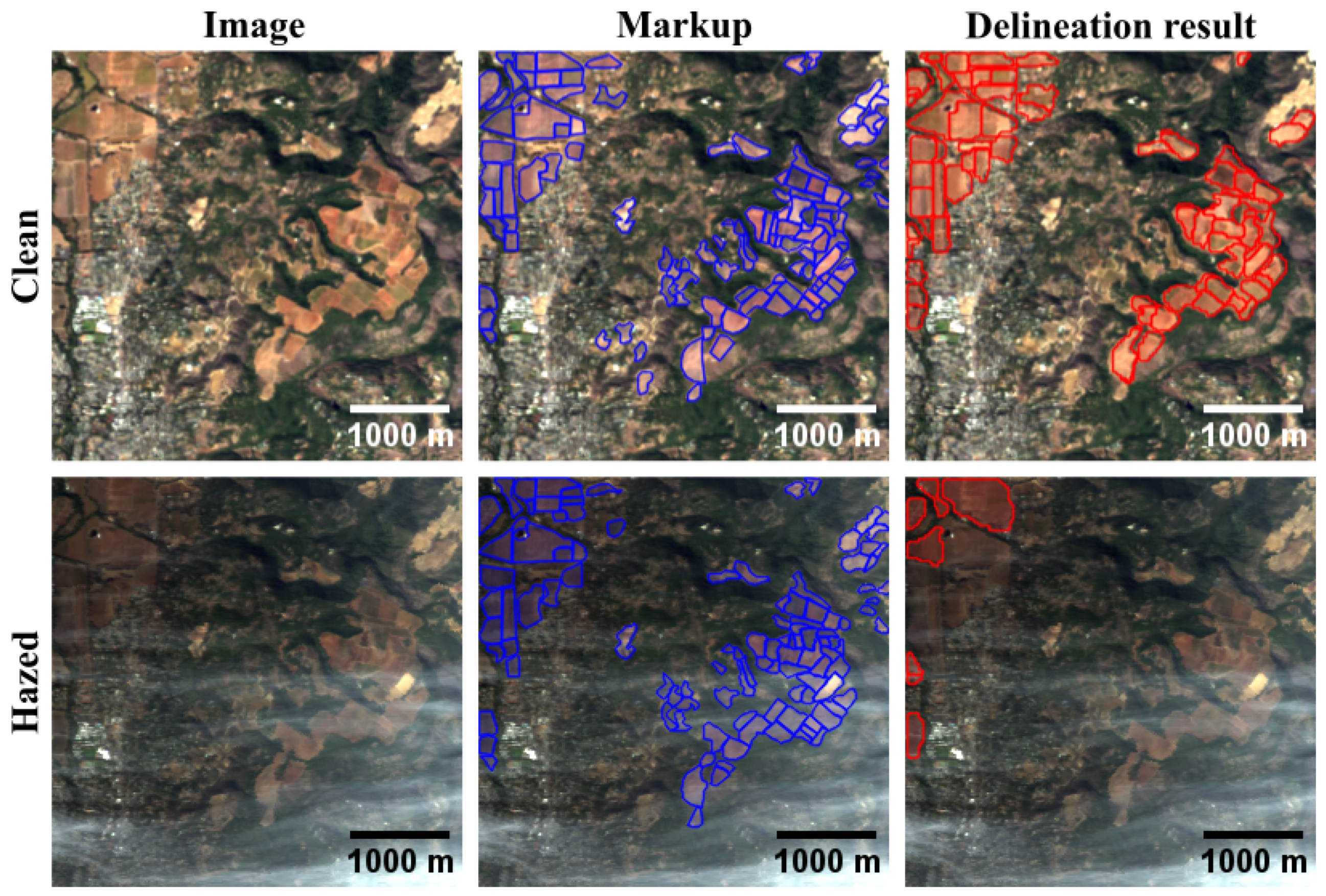
Figure 7.
Results of applying the DA agricultural field delineation method to clean and hazy RGB images from the RRealHyperPDID dataset generated using the CSNC method. The blue delineation mask represents manual annotations, while the red delineation mask corresponds to the algorithm’s output.
Figure 7.
Results of applying the DA agricultural field delineation method to clean and hazy RGB images from the RRealHyperPDID dataset generated using the CSNC method. The blue delineation mask represents manual annotations, while the red delineation mask corresponds to the algorithm’s output.
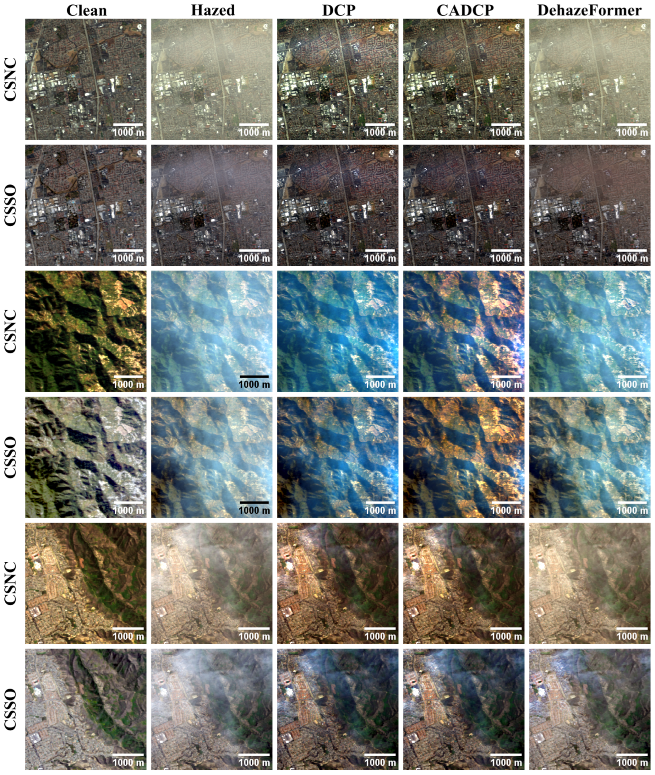
Figure 8.
Examples of RGB dehazing results obtained using the CSNC and CSSO RGB synthesis methods.
Figure 8.
Examples of RGB dehazing results obtained using the CSNC and CSSO RGB synthesis methods.
Figure 9.
RGB visualization comparison of HS dehazing methods trained on the HyperDehazing synthetic training set and evaluated on the test set.
Figure 9.
RGB visualization comparison of HS dehazing methods trained on the HyperDehazing synthetic training set and evaluated on the test set.
Figure 10.
Spectral reconstruction performance for various HS dehazing methods on the HyperDehazing test set. The red plus sign indicates the pixel location for which the spectral reconstruction is shown.
Figure 10.
Spectral reconstruction performance for various HS dehazing methods on the HyperDehazing test set. The red plus sign indicates the pixel location for which the spectral reconstruction is shown.
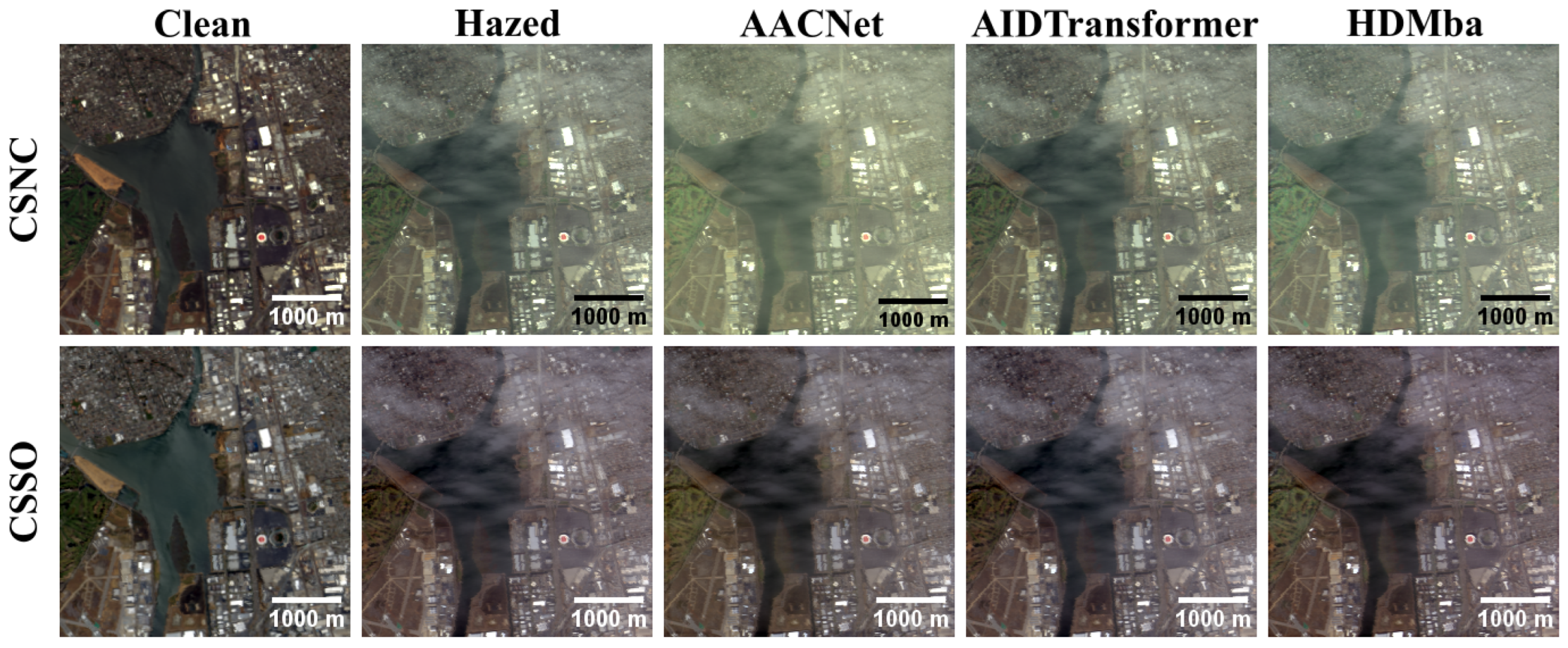
Figure 11.
RGB visualization comparison of HS dehazing methods trained on the HyperDehazing synthetic dataset and tested on the RRealHyperPDID real-world dataset.
Figure 11.
RGB visualization comparison of HS dehazing methods trained on the HyperDehazing synthetic dataset and tested on the RRealHyperPDID real-world dataset.
Figure 12.
Spectral reconstruction performance of HS dehazing methods on the RRealHyperPDID dataset. The red plus sign indicates the pixel location for which the spectral reconstruction is shown.
Figure 12.
Spectral reconstruction performance of HS dehazing methods on the RRealHyperPDID dataset. The red plus sign indicates the pixel location for which the spectral reconstruction is shown.
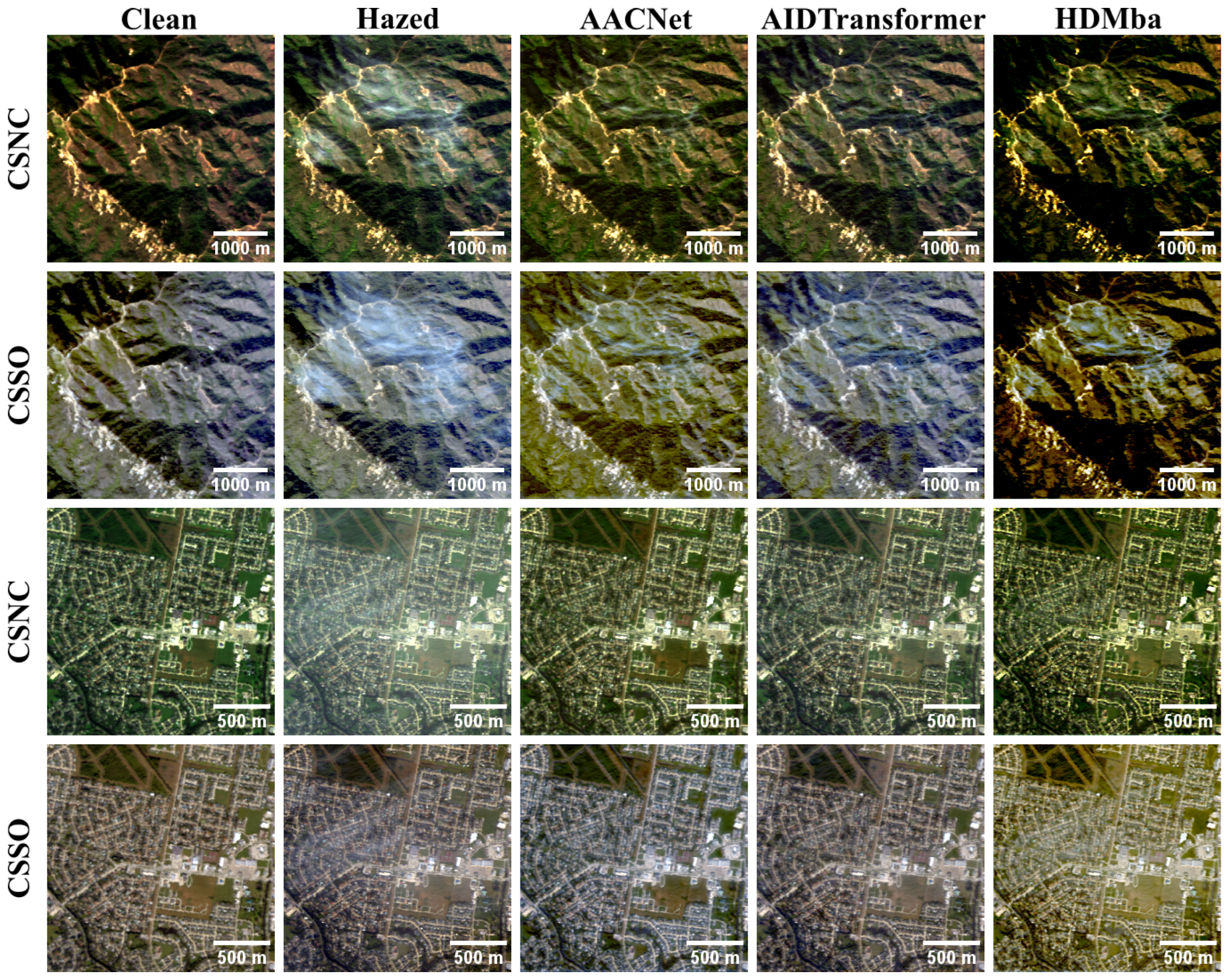
Figure 13.
RGB visualization comparison of HS dehazing methods trained on the RSyntHyperPDID synthetic dataset and tested on the RRealHyperPDID real-world dataset.
Figure 13.
RGB visualization comparison of HS dehazing methods trained on the RSyntHyperPDID synthetic dataset and tested on the RRealHyperPDID real-world dataset.
Figure 14.
Spectral reconstruction performance of HS dehazing methods trained on the RSyntHyperPDID dataset. The red plus sign indicates the pixel location for which the spectral reconstruction is shown.
Figure 14.
Spectral reconstruction performance of HS dehazing methods trained on the RSyntHyperPDID dataset. The red plus sign indicates the pixel location for which the spectral reconstruction is shown.
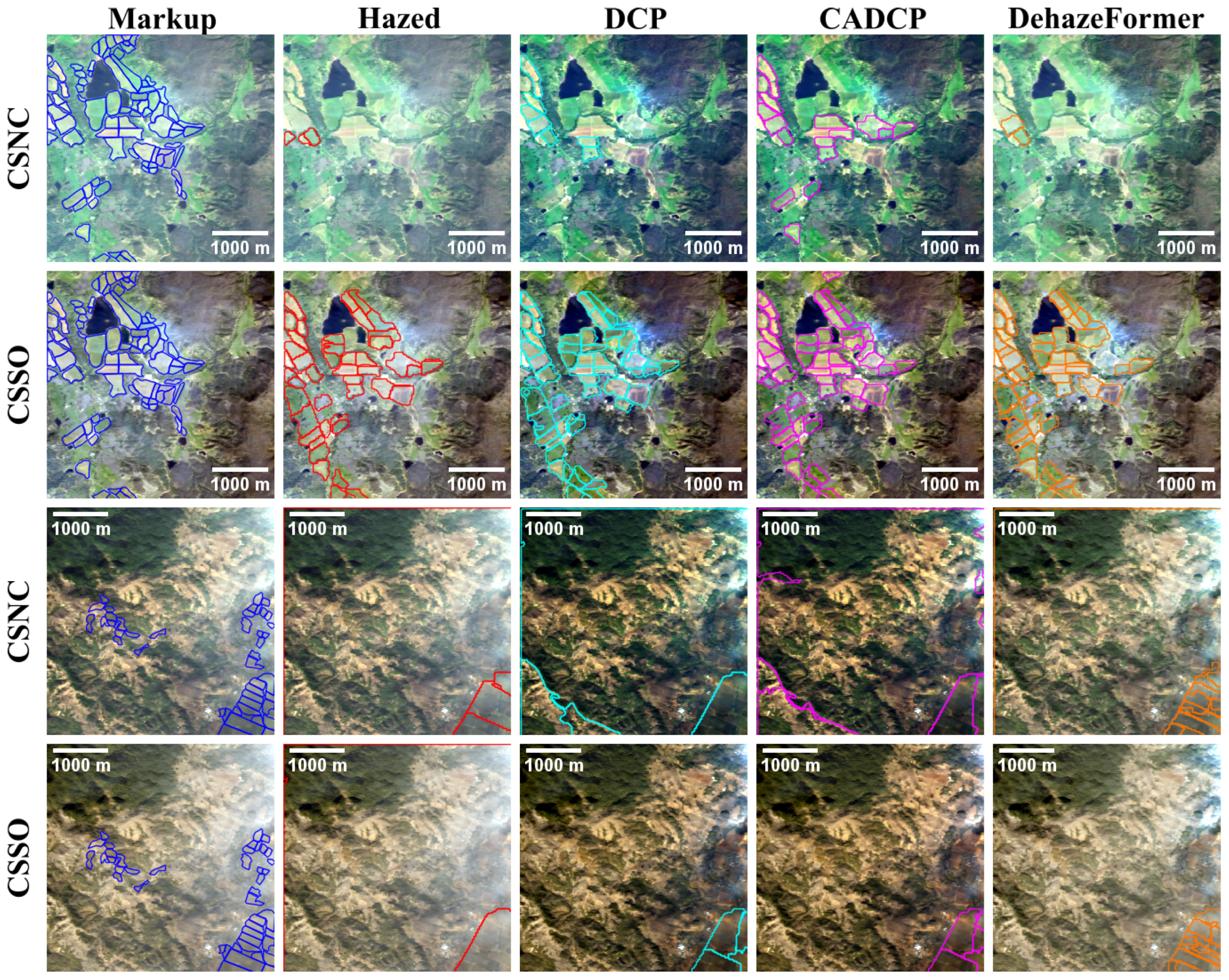
Figure 15.
Results of applying the DA method to hazy and dehazed images generated using the CSNC and CSSO RGB synthesis methods. The colors of delineation masks indicate DA results applied to images processed by different dehazing methods.
Figure 15.
Results of applying the DA method to hazy and dehazed images generated using the CSNC and CSSO RGB synthesis methods. The colors of delineation masks indicate DA results applied to images processed by different dehazing methods.
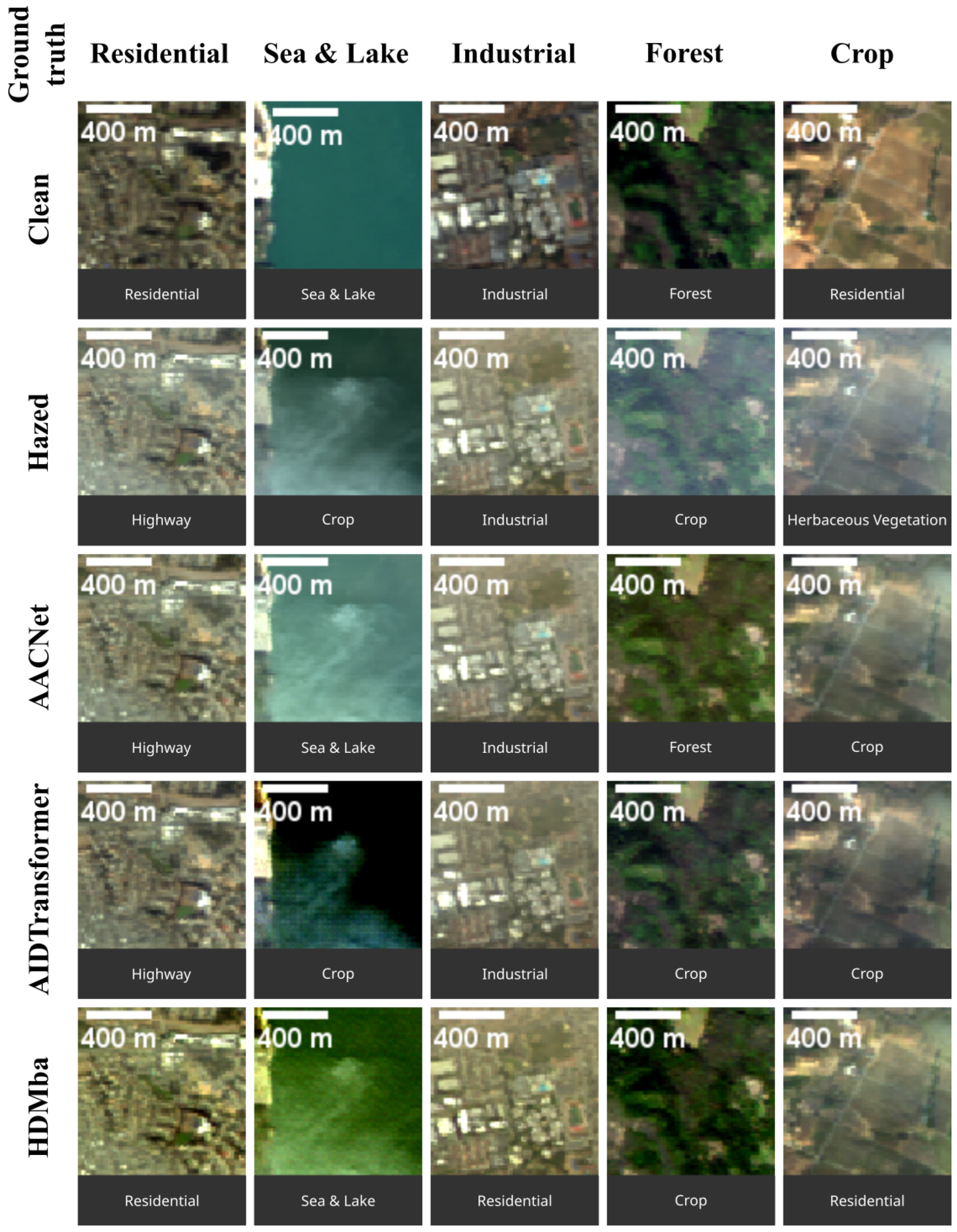
Figure 16.
LULC classification results for hazy and dehazed images. The first row shows the ground truth class for each scene. The label below each image patch indicates the class predicted by the classification algorithm.
Figure 16.
LULC classification results for hazy and dehazed images. The first row shows the ground truth class for each scene. The label below each image patch indicates the class predicted by the classification algorithm.
Table 1.
Comparison of the proposed datasets, RRealHyperPDID and RSyntHyperPDID, with existing remote sensing dehazing datasets.
Table 1.
Comparison of the proposed datasets, RRealHyperPDID and RSyntHyperPDID, with existing remote sensing dehazing datasets.
| Dataset | Size | Real/Synthetic | Paired | Resolution | Image Type |
|---|
| RRSHID [22] | 3053 | Real | Yes | 256 × 256 | RGB |
| RS-Haze [14] | 51,300 | Synthetic | Yes | 512 × 512 | RGB |
| HyperDehazing [24] | 2000 | Synthetic | Yes | 512 × 512 | Hyperspectral |
| HyperDehazing [24] | 70 | Real | No | 512 × 512 | Hyperspectral |
| HDD [25] | 40 | Real | No | 512 × 512 | Hyperspectral |
| RRealHyperPDID | 110 | Real | Yes | 256 × 256 | Hyperspectral |
| RSyntHyperPDID | 2616 | Synthetic | Yes | 256 × 256 | Hyperspectral |
Table 2.
Comparison of the DA agricultural field delineation method results for clean and hazy RGB images.
Table 2.
Comparison of the DA agricultural field delineation method results for clean and hazy RGB images.
| Data | DICE | DICEobj | Number of Images |
|---|
| clean (CSNC) | 57.17 | 25.46 | 52 |
| hazed (CSNC) | 38.59 | 15.93 | 34 |
| clean (CSSO) | 51.24 | 22.8 | 52 |
| hazed (CSSO) | 42.61 | 20.93 | 34 |
Table 3.
Results of various RGB dehazing methods applied to RRealHyperPDID images (CSNC RGB synthesis method). Entries show the mean values with 95% bootstrap confidence intervals (bias-corrected and accelerated, BCa). Bold indicates the best result, and underlined indicates the second-best.
Table 3.
Results of various RGB dehazing methods applied to RRealHyperPDID images (CSNC RGB synthesis method). Entries show the mean values with 95% bootstrap confidence intervals (bias-corrected and accelerated, BCa). Bold indicates the best result, and underlined indicates the second-best.
| Method | PSNR ↑ | SSIM ↑ | SAM ↓ | DISTS ↓ | LPIPS ↓ | CDproLab ↓ |
|---|
| No dehazing | 14.10 ± 0.54 | 0.605 ± 0.017 | 0.193 ± 0.019 | 0.231 ± 0.008 | 0.366 ± 0.013 | 0.160 ± 0.015 |
| DCP [6] | 16.81 ± 0.51 | 0.631 ± 0.020 | 0.234 ± 0.024 | 0.203 ± 0.007 | 0.359 ± 0.014 | 0.184 ± 0.016 |
| CADCP [10] | 17.00 ± 0.51 | 0.635 ± 0.020 | 0.217 ± 0.023 | 0.198 ± 0.007 | 0.352 ± 0.014 | 0.171 ± 0.015 |
| DehazeFormer [14] | 15.56 ± 0.49 | 0.631 ± 0.017 | 0.180 ± 0.020 | 0.208 ± 0.007 | 0.352 ± 0.013 | 0.147 ± 0.015 |
Table 4.
Results of various RGB dehazing methods applied to RRealHyperPDID images (CSSO RGB synthesis method). Entries show the mean values with 95% bootstrap confidence intervals (bias-corrected and accelerated, BCa). Bold indicates the best result, and underlined indicates the second-best.
Table 4.
Results of various RGB dehazing methods applied to RRealHyperPDID images (CSSO RGB synthesis method). Entries show the mean values with 95% bootstrap confidence intervals (bias-corrected and accelerated, BCa). Bold indicates the best result, and underlined indicates the second-best.
| Method | PSNR ↑ | SSIM ↑ | SAM ↓ | DIST ↓ | LPIPS ↓ | CDproLab ↓ |
|---|
| No dehazing | 16.71 ± 0.52 | 0.655 ± 0.016 | 0.142 ± 0.013 | 0.215 ± 0.009 | 0.378 ± 0.015 | 0.130 ± 0.011 |
| DCP [6] | 15.48 ± 0.46 | 0.602 ± 0.015 | 0.214 ± 0.015 | 0.216 ± 0.007 | 0.383 ± 0.015 | 0.178 ± 0.012 |
| CADCP [10] | 15.53 ± 0.45 | 0.603 ± 0.015 | 0.209 ± 0.014 | 0.215 ± 0.007 | 0.381 ± 0.015 | 0.175 ± 0.012 |
| DehazeFormer [14] | 17.42 ± 0.50 | 0.657 ± 0.016 | 0.155 ± 0.014 | 0.198 ± 0.008 | 0.366 ± 0.016 | 0.137 ± 0.013 |
Table 5.
Expert-based scores of RGB dehazing methods on the RRealHyperPDID dataset.
Table 5.
Expert-based scores of RGB dehazing methods on the RRealHyperPDID dataset.
| Method | CSNC | CSSO |
|---|
| No dehazing | 0.0005 | 0.0007 |
| DCP | 0.3068 | 0.3558 |
| CADCP | 0.6762 | 0.6027 |
| DehazeFormer | 0.0165 | 0.0408 |
Table 6.
Kendall correlation coefficients between metric-based and expert rankings of dehazing algorithms, shown separately for close and other scenes of RRealHyperPDID.
Table 6.
Kendall correlation coefficients between metric-based and expert rankings of dehazing algorithms, shown separately for close and other scenes of RRealHyperPDID.
| Close Scenes | | Other Scenes |
|---|
| PSNR | SSIM | SAM | DISTS | LPIPS | | PSNR | SSIM | SAM | DISTS | LPIPS |
|---|
| | | | | | CSNC | | | | | |
| 0.91 | 0.91 | - | 1 | - | | 1 | - | −0.33 | - | −0.18 |
| | | | | | CSSO | | | | | |
| −0.60 | −0.60 | −0.80 | 0.18 | - | | −0.55 | −0.91 | −0.91 | - | −0.55 |
Table 7.
Reproduction of neural network HSI dehazing results on the HyperDehazing test set. Results for hazy images were not provided in [
18].
Table 7.
Reproduction of neural network HSI dehazing results on the HyperDehazing test set. Results for hazy images were not provided in [
18].
| | [18] Results | Our Results |
|---|
| Method | PSNR ↑ | SSIM ↑ | SAM ↓ | PSNR ↑ | SSIM ↑ | SAM ↓ |
|---|
| No dehazing | - | - | - | 32.81 | 0.9513 | 0.0348 |
| AACNet [23] | 37.43 | 0.9734 | 0.0425 | 40.44 | 0.9572 | 0.0189 |
| AIDTransformer [15] | 35.47 | 0.9723 | 0.0401 | 38.13 | 0.9553 | 0.0262 |
| HDMba [18] | 38.13 | 0.9763 | 0.0382 | 36.16 | 0.9525 | 0.0352 |
Table 8.
Results of HS dehazing methods on the RRealHyperPDID dataset. Models were trained on the HyperDehazing training set. Entries show the mean values with 95% bootstrap confidence intervals (bias-corrected and accelerated, BCa). Bold indicates the best result, and underlined indicates the second-best.
| Method | PSNR ↑ | SSIM ↑ | SAM ↓ |
|---|
| No dehazing | 25.49 ± 0.73 | 0.685 ± 0.022 | 0.196 ± 0.016 |
| AACNet [23] | 19.00 ± 0.52 | 0.517 ± 0.024 | 0.364 ± 0.021 |
| AIDTransformer [15] | 25.16 ± 0.73 | 0.682 ± 0.023 | 0.202 ± 0.017 |
| HDMba [18] | 22.19 ± 0.58 | 0.616 ± 0.025 | 0.280 ± 0.019 |
Table 9.
Results of neural network-based HS dehazing methods on the validation subset of the synthetic-haze RSyntHyperPDID and real-haze RRealHyperPDID. Models were trained on the RSyntHyperPDID training set. Entries show the mean values with 95% bootstrap confidence intervals (bias-corrected and accelerated, BCa). Bold indicates the best result, and underlined indicates the second-best.
| | RSyntHyperPDID Test | RRealHyperPDID |
|---|
| Method | PSNR ↑ | SSIM ↑ | SAM ↓ | PSNR ↑ | SSIM ↑ | SAM ↓ |
|---|
| No dehazing | 22.61 ± 0.55 | 0.911 ± 0.009 | 0.133 ± 0.006 | 26.45 ± 0.74 | 0.695 ± 0.022 | 0.200 ± 0.016 |
| AACNet [23] | 34.19 ± 0.38 | 0.972 ± 0.002 | 0.048 ± 0.003 | 27.82 ± 0.75 | 0.688 ± 0.021 | 0.182 ± 0.019 |
| AIDTransformer [15] | 30.54 ± 0.57 | 0.955 ± 0.005 | 0.064 ± 0.004 | 28.09 ± 0.65 | 0.628 ± 0.016 | 0.214 ± 0.027 |
| HDMba [18] | 27.90 ± 0.57 | 0.941 ± 0.007 | 0.086 ± 0.006 | 27.65 ± 0.65 | 0.583 ± 0.015 | 0.237 ± 0.030 |
Table 10.
Comparison of DA results for hazy and dehazed images processed with DCP, CADCP, and DehazeFormer algorithms.
Table 10.
Comparison of DA results for hazy and dehazed images processed with DCP, CADCP, and DehazeFormer algorithms.
| | CSNC | CSSO |
|---|
| Data | DICE ↑ | DICEobj ↑ | DICE ↑ | DICEobj ↑ |
|---|
| hazed | 38.59 | 15.93 | 42.61 | 20.93 |
| DCP [6] | 43.16 | 18.01 | 47.22 | 22.88 |
| CADCP [10] | 45.95 | 19.36 | 47.35 | 21.45 |
| DehazeFormer [14] | 46.92 | 20.55 | 50.31 | 23.22 |
| clean | 57.17 | 25.46 | 51.24 | 22.8 |
Table 11.
LULC classification results on MS images synthesized from the RRealHyperPDID dataset.
Table 11.
LULC classification results on MS images synthesized from the RRealHyperPDID dataset.
| Method | Accuracy |
|---|
| clean | 74.56% |
| hazed | 56.29% |
| AIDTransformer | 59.86% |
| AACNet | 62.47% |
| HDMba | 56.29% |


