Article

Lightweight Statistical and Texture Feature Approach for Breast Thermogram Analysis †

by
Ana P. Romero-Carmona
,
Jose J. Rangel-Magdaleno
,
Francisco J. Renero-Carrillo
,
Juan M. Ramirez-Cortes
and
Hayde Peregrina-Barreto
*
Instituto Nacional de Astrofísica, Óptica y Electrónica (INAOE) Tonantzintla, Puebla 72840, Mexico
*
Author to whom correspondence should be addressed.
This paper is an extended version of our paper published in Romero-Carmona, A.; Peregrina-Barreto, H.; Renero-Carrillo, F. Breast Cancer Thermography Classification with a Reduced Description and Machine Learning. In Proceedings of the 2024 IEEE International Autumn Meeting on Power, Electronics and Computing (ROPEC), Ixtapa, Guerrero, México, 11–13 November 2024; pp. 1–6.
J. Imaging 2025, 11(10), 358; https://doi.org/10.3390/jimaging11100358
Submission received: 30 August 2025 / Revised: 9 October 2025 / Accepted: 10 October 2025 / Published: 13 October 2025
(This article belongs to the Section Medical Imaging)

Abstract

Breast cancer is the most commonly diagnosed cancer in women globally and represents the leading cause of mortality related to malignant tumors. Currently, healthcare professionals are focused on developing and implementing innovative techniques to improve the early detection of this disease. Thermography, studied as a complementary method to traditional approaches, captures infrared radiation emitted by tissues and converts it into data about skin surface temperature. During tumor development, angiogenesis occurs, increasing blood flow to support tumor growth, which raises the surface temperature in the affected area. Automatic classification techniques have been explored to analyze thermographic images and develop an optimal classification tool to identify thermal anomalies. This study aims to design a concise description using statistical and texture features to accurately classify thermograms as control or highly probable to be cancer (with thermal anomalies). The importance of employing a short description lies in facilitating interpretation by medical professionals. In contrast, a characterization based on a large number of variables could make it more challenging to identify which values differentiate the thermograms between groups, thereby complicating the explanation of results to patients. A maximum accuracy of 91.97% was achieved by applying only seven features and using a Coarse Decision Tree (DT) classifier and robust Machine Learning (ML) model, which demonstrated competitive performance compared with previously reported studies.

1. Introduction

Breast cancer is a malignant disease characterized by the uncontrolled growth of cancerous cells in breast tissue, leading to the formation of tumors. Over time, these tumors can invade surrounding tissues and spread to other parts of the body, a process known as metastasis [1]. Globally, breast cancer is the most commonly diagnosed cancer in women and represents the leading cause of death from malignant tumors. In 2020, approximately 685,000 deaths were attributed to this disease, making it the primary cause of cancer-related mortality among women [2,3]. Over the years, innovative techniques have been developed for the diagnosis and treatment of breast cancer, contributing to a reduction in the overall mortality rate. However, early detection remains one of the primary challenges in the healthcare field [4]. Early detection is crucial for the timely implementation of treatments and improving survival rates. Currently, the most widely used technologies for breast cancer detection include mammography, tomosynthesis, ultrasound, and magnetic resonance imaging [5]. However, the use of radiation and high costs are limitations that must be taken into consideration. These limitations have driven the development of new complementary tools to improve early breast cancer detection.
Over the past few decades, the use of infrared thermography in medical applications has been extensively studied. Thanks to advances in science and technology, the sensitivity of this technique has increased significantly, enabling it to detect subtle temperature variations [6]. The infrared radiation emitted by the body is captured through a thermal camera, allowing for the measurement of these thermal changes. Thus, thermography provides a fast, non-invasive, painless, and low-cost alternative [7,8,9]. Its use as a complementary diagnostic tool has been explored in various medical fields. In patients with rheumatic diseases, thermal changes were associated with areas of pain or swelling [10]. In the diagnosis and monitoring of peripheral vascular diseases that affect the peripheral circulatory system, it has been used to study varicose veins and diabetic foot [11]. In the context of respiratory diseases, thermography has proven helpful in identifying the intersegmental plane of the lungs, which facilitates pulmonary surgeries [12]. In oncology, it has been employed to detect thermal anomalies related to breast cancer, skin cancer, and metastasis of head and neck cancer, among others [13,14,15].
In 1956, Lawson identified a correlation between increased skin temperature and the presence of breast carcinoma, suggesting it as an indicator of anomalies associated with this disease. Cancerous cells require a greater supply of oxygen and nutrients to grow and propagate, which triggers a process called angiogenesis—the formation of new blood vessels around tumors. This increase in blood flow and metabolism within the tumor raises the temperature of the affected area compared with the surrounding tissues. As a result of these findings, the FDA approved thermography as a complementary tool for assessing the risk of breast tumors. According to the American College of Clinical Thermology, thermography has several advantages: The results are unaffected by breast tissue density, the presence of implants, or hormonal changes. Additionally, it is safe for continuous use, as it does not expose patients to radiation.
Nevertheless, interpreting thermographic images (thermograms) is challenging due to the wide variability in temperature distributions. To address this, computer vision and Machine Learning (ML) methods have been applied for anomaly detection, diagnosis, and surgical guidance [16]. In breast cancer research, ML, Deep Learning (DL), and Transfer Learning approaches have been used to classify thermograms as healthy or cancerous, improving diagnostic efficiency. These algorithms can support clinical decision-making and potentially enhance patient survival [17]. Recent studies have explored combining thermography with ML for breast cancer detection [18]. This approach can reduce human subjectivity by enabling automated interpretation of thermal images. However, many ML- or DL-based methods rely on a large number of features, which can limit interpretability for medical professionals. Thus, there is a need for approaches that use a smaller set of optimal features while maintaining classification accuracy.
This study proposes a descriptive framework to facilitate the interpretation of temperature information in breast thermograms. While elevated temperature and changes in its distribution are associated with abnormal behavior in the breast region, such variations do not consistently follow a spatial pattern, making their characterization challenging. To address this, statistical and textural features were computed, and the most informative ones were selected to provide a concise yet effective description of healthy and cancerous thermograms. Feature analysis was restricted to the breast region to minimize interference from surrounding anatomical areas, and each breast was evaluated individually, given the potential for intra-subject differences. The proposed description was evaluated using four classifiers, achieving an accuracy of 91.97 % . Moreover, through the analysis of the 95% confidence intervals of the performance metrics using the bootstrap and McNemar tests, it was demonstrated that the proposed description remains consistent regardless of the classifier used. These results demonstrate that a lightweight feature set, combined with classical descriptors, enables the accurate classification of breast thermograms, offering a competitive alternative to current state-of-the-art methods.

2. Materials and Methods

2.1. Dataset

To develop this work, a reference thermographic image database was used. The Dataset for Mastology Research (DMR) is a publicly available database developed by Federal Fluminense University in Brazil and has been widely referenced in the scientific literature. The DMR contains a set of thermographic images corresponding to patients classified as healthy or diseased. These images were captured using an FLIR SC-620 infrared camera, which offers a thermal sensitivity of 0.04 °C and a resolution of 640 × 480 pixels [19]. This database has been particularly used in research focused on the early detection of breast cancer, making it relevant for the present study. To mitigate redundancy and reduce the risk of overoptimistic bias in performance estimates, images with similar viewing angles and no significant differences were excluded from analysis. The evaluation was restricted to front-view images, which offer the most comprehensive visualization of the breast region. Furthermore, thermogram analysis was performed using temperature values extracted from radiometric files, as color palettes merely provide perceptual contrast without modifying the quantitative information. Taking these considerations into account, 141 thermograms were selected, of which 99 corresponded to the control group and 42 to the group of patients with cancer confirmed by biopsy. Figure 1 shows some samples of both groups. In order to maintain consistency in the representation of thermograms, the information is presented using the same temperature scale in a range of [20, 36] °C.

2.2. ROI Extraction

In clinical thermograms, certain areas often exhibit elevated temperatures that do not necessarily indicate abnormality. For instance, the armpits and neck typically register higher temperatures compared with the breast region. However, in the context of breast temperatures, a similar pattern may indicate an abnormality. Therefore, it was decided to perform image segmentation to separate the regions of interest (ROIs) for analysis. During the segmentation process, a set of binary masks was manually created to separate the breast region from the background, allowing the application of specific local operations on the images. For each thermogram, a binary mask covering the area of both breasts was generated (Figure 2). Subsequently, each mask was divided into two by making a vertical division in the middle of both breasts to obtain two new masks corresponding to each breast individually. This decision was made after a series of tests revealed that analyzing the breasts individually provided a more precise approach and more robust results. This is because the thermal conditions of each breast can vary significantly; for example, some patients with temperature anomalies may present such behavior in only one breast.

2.3. Feature Extraction

One of the key processes for classification is image analysis, where it is essential to identify and quantify specific features that are relevant for accurate classification. By focusing solely on the data that most precisely describes the content of the image, the complexity of the process is reduced, allowing the analysis to focus on critical aspects such as edges, textures, shapes, and patterns, among others. In general, two main types of features can be extracted: statistical features and texture features. Statistical features describe the distribution of pixel values in the image, while texture features capture the variability and spatial patterns present in the image.
In this study, both types of features were employed to improve classification results by leveraging the relevant aspects that thermograms can contribute to this task. For feature selection, a thorough review of the existing literature related to the classification of thermographic images was conducted. The goal was to rigorously identify those features that could optimize the efficiency of the classification methods used. Based on the literature review, the following features were selected [20,21,22,23,24]:
(a)
Statistical features
  • Mean ( μ ): The average intensity value of the pixels that make up an image, indicating the mean color or brightness value in the image, where T ( x , y ) represents the temperature at position ( x , y ) in an image of size M × N .
    μ = 1 M N x = 0 M 1 y = 0 N 1 T ( x , y )
  • Standard deviation ( σ ) and variance ( σ 2 ): Indicate the dispersion of values in an image. Variance measures how much the pixel values deviate from the overall mean of these values in the image. The standard deviation, which is the square root of the variance, provides a more direct measure of dispersion. Both metrics offer insights into the variability of texture and contrast in the image.
    σ = 1 M N x = 0 M 1 y = 0 N 1 ( T ( x , y ) μ ) 2
  • Skewness ( γ ): A measure that indicates the degree of symmetry in the pixel distribution, with a particular emphasis on asymmetry. If the intensity values in an image are concentrated at one end of the spectrum, it suggests asymmetry, which may reveal specific patterns or features in the image.
    γ = μ m e d i a n σ
  • Kurtosis (k): A quantitative metric that characterizes the shape of the pixel distribution. It is utilized in image analysis to detect underlying patterns that may not be discernible through visual inspection.
    k = E ( x μ ) 4 σ 4
  • Entropy (H): A measure of randomness in the distribution of pixel values in an image. It is a tool that provides a representative value of the complexity in a specific section of the image, where G is the number of gray levels.
    H = i = 1 G p i log 2 ( p i )
  • Maximum and minimum values: Values that represent the extremes of the range of pixel intensities in an image. In the case of thermographic images, the minimum value indicates the lowest intensity (temperature) detected, while the maximum value indicates the highest intensity.
  • Coefficient of variation ( C V ): A measure that evaluates the deviations of pixels from their mean and the dispersion among them. In a thermographic image, the coefficient of variation indicates the variability of temperature in the image.
    C V = σ μ × 100
(b)
Texture features
Features were obtained using the Gray-Level Co-occurrence Matrix (GLCM), which describes the frequency with which one gray level appears near another gray level within a small region of the image. In other words, the GLCM provides information about the distribution of gray levels relative to each other in a specific area of the image, thus allowing the observation of pixel clustering patterns [23,25].
For the construction of the co-occurrence matrices, gray levels were considered in the range of [ 0 , 255 ] . The co-occurrences between the central pixel and those at a distance of one were analyzed, considering four directions { 0 , 45 , 90 , 135 } . The matrices obtained in each direction were integrated for an integral analysis of changes in all directions. From the resulting matrix, the properties of homogeneity, contrast, correlation, and energy were extracted as described below.
  • Homogeneity: A measure that indicates how uniform the distribution of pixel values is within a region of an image. High homogeneity suggests that the gray levels in the image are very similar to each other.
    Homogeneity = x , y 1 1 + ( x y ) 2 T ( x , y )
  • Contrast: It measures the difference in intensity between the pixels of an image. A higher contrast indicates that there are significant differences in pixel intensities.
    Contrast = x , y ( x y ) 2 T ( x , y )
  • Correlation: A measure that describes the relationship between pixel values, helping to identify patterns or trends in their arrangement. High contrast indicates that the pixel values are uniformly distributed in the GLCM.
    Correlation = x , y ( x μ x ) ( y μ y ) T ( x , y ) σ x σ y
  • Energy (E): A measure that describes the variation in intensity between pixels, taking into account how factors such as color, brightness, magnitude, shadows, or textures change as one moves from one pixel to another. In an image, areas with edges or textured patterns contain higher energy, indicating greater visual complexity. In thermographic images, energy is calculated by summing the intensities (temperatures) of each pixel in the image, as shown in Equation (10).
    E = x = 0 M 1 y = 0 N 1 T ( x , y )

2.4. Feature Selection

To achieve a more efficient and effective classification process, feature reduction can be a valuable tool, as it helps confirm the relevance of each feature used. A statistical test was conducted to verify that the selected features provided meaningful information for image classification. The Student’s t-test was chosen, which is used to determine if there is a significant difference between the means of two groups [26]. In this context, it will be applied to identify features that genuinely help differentiate between images with a higher probability of cancer and those with more similarity to the control.
The first step in this process is to establish the null and alternative hypotheses. The null hypothesis states that there is no significant difference between the means of the two classes, while the alternative hypothesis suggests that there is a significant difference. Next, the data should be divided into two subsets corresponding to each of the two existing classes, labeled as C 1 and C 2 , with samples being represented by X 1 and X 2 , respectively. Finally, for each feature i, the mean in both classes is calculated using Equation (11).
X ¯ i , C 1 = 1 n 1 j = 1 n 1 X i , j , C i X ¯ i , C 2 = 1 n 2 j = 1 n 2 X i , j , C 2
where x ¯ i , C 1 and x ¯ i , C 2 represent the mean of feature i in classes C 1 and C 2 , respectively; n 1 and n 2 represent the number of samples in classes C 1 and C 2 , respectively. x i , j , C 1 and x i , j , C 2 represent the value of feature i in sample j for classes C 1 and C 2 , respectively.
To conduct this test, it is essential to calculate the mean ( μ ) and variance ( σ 2 ) of each feature i in both classes. The t-statistic is determined for each feature i using Equation (12). Subsequently, using t-distribution tables, which provide critical values for the t-distribution at various significance levels and degrees of freedom, the corresponding p-value for each feature is determined. This p-value indicates whether the null hypothesis is accepted, meaning that there is no significant difference between the means of the two classes for that particular feature. In this study, a significance level of 0.05 was used, so features with a p-value lower than the established significance level are considered relevant and useful for classification [27].
t i = X ¯ i , C 1 X ¯ i , C 2 σ 1 i 2 n 1 + σ 2 i 2 n 2

2.5. Model Validation

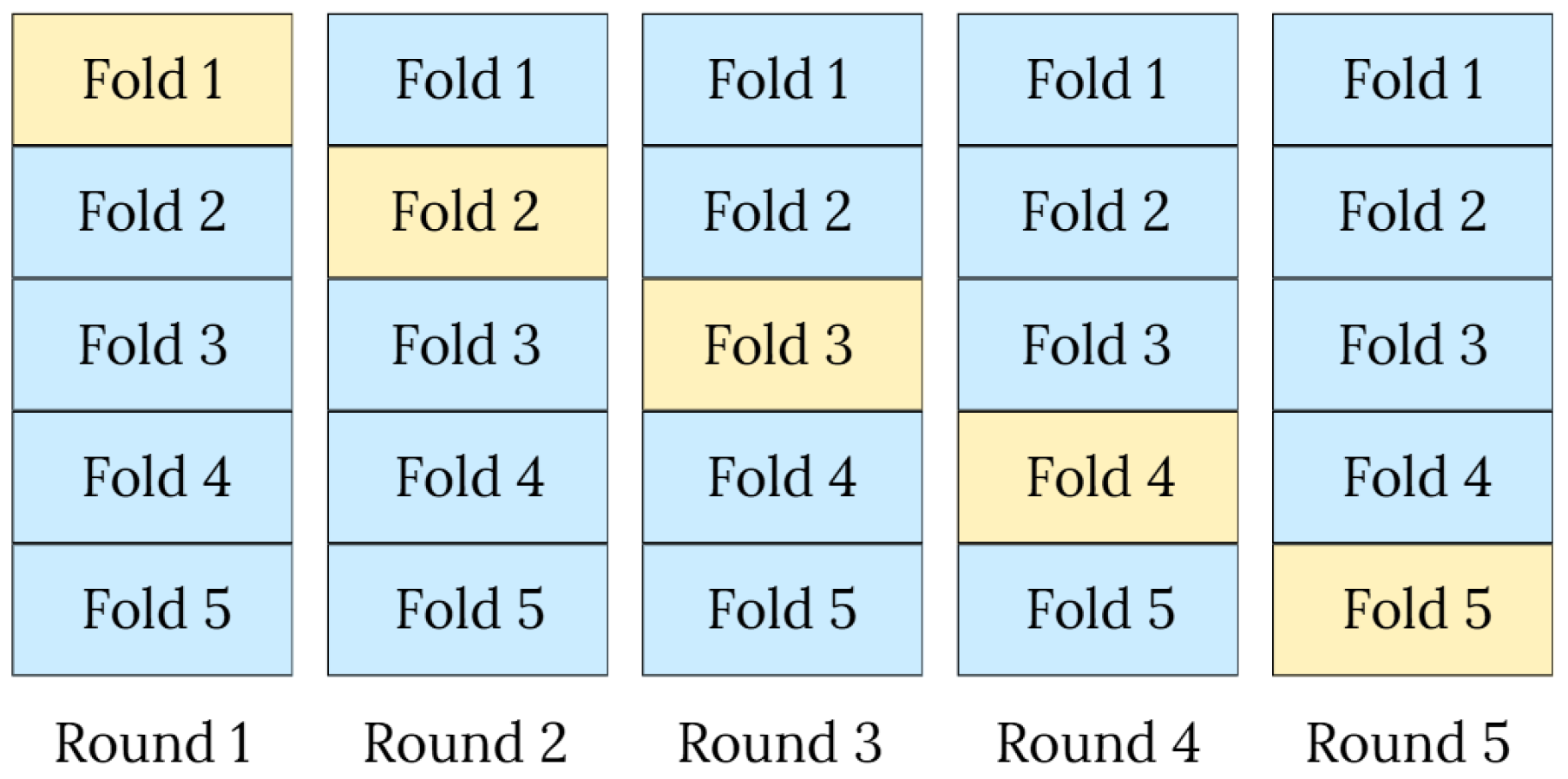
To evaluate the performance of classifiers, a stratified cross-validation was employed to assess the replicability of the results, as well as the generalization and stability of the findings. This approach has proven helpful for imbalanced datasets since a purely random partition could lead to folds with insufficient representation of the minority class [28]. In stratified cross-validation, the dataset is divided into k folds in a way that preserves the overall class distribution of the complete dataset within each fold. For example, if the dataset contains 80% of samples from class 0 and 20% from class 1, each fold will approximately maintain this same proportion.
At each iteration, k − 1 folds are selected for training, and the remaining fold is used for testing. Thus, in each round, a model is trained and fitted so that the training and test folds differ each time, as illustrated in Figure 3. This strategy enables the representation of both majority and minority classes in each fold, thereby reducing variance and bias in performance metrics.

2.6. Classification Methods

Although CNNs or DL models have also been employed in this context, they require extensive samples to achieve robust learning and avoid overfitting [29]. Particularly, in medical datasets, the scarcity of labeled data along with the importance of clinical variability poses an important consideration for applying these models. On the other hand, traditional ML is an appropriate approach when there is a limited set of data available [30,31,32]. To accomplish this classification task, four ML models were employed: SVM (quadratic and linear), LR, and DT.
The Support Vector Machine (SVM) is a supervised learning algorithm that operates by mapping data to a high-dimensional feature space using kernel functions, enabling the classification of data into distinct categories. SVM aims to identify a hyperplane that separates the data of different classes within the feature space, choosing the hyperplane that maximizes the minimum distance between the hyperplane itself and the closest data points from each class. In this study, two variants of the SVM algorithm were utilized: linear SVM and quadratic SVM. The primary distinction between them lies in the shape of the hyperplane used to separate the classes, which could be a straight line or a quadratic curve [33]. The Logistic Regression (LR) algorithm performs binary classification tasks by predicting the probability of an outcome or observation expressed in a binary value. It is widely used in predictive models, where it estimates the likelihood that an instance belongs to a specific category or not. For the purposes of this study, the categories will be associated with thermograms that have or do not have [34,35] them. The Coarse Tree (CT) method is a supervised learning approach based on DT that employs iterative segmentation of the feature space to create simpler regions. Additionally, it tends to generalize more, which reduces the likelihood of overfitting the training data [36].

3. Experimental Results

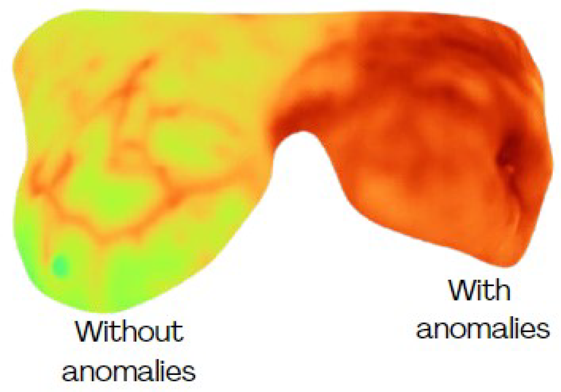
Thermograms were analyzed by focusing on the breast region only, i.e., extracting the area indicated by the binary mask (Figure 2). Nevertheless, a high degree of variability can be present among the breasts of the same subject (Figure 4), which can affect their evaluation. Therefore, this study considers each breast as an individual case. Some individual samples were removed when they presented low resolution (high blurring) or a breast amputation had occurred. A total of 265 individual thermographic samples were generated, comprising 71 samples from the cancer group and 194 from the control group. For model validation, a stratified 5-fold cross-validation was applied to test each classifier.
For feature selection, the Student’s t-test was applied to the 14 initially selected features, considering as optimal those with a p-value <   0.05 . According to the p-value texture features of homogeneity, contrast, and correlation and four statistical features of entropy, min, and max values, were selected from Table 1. These seven features were used as input variables in the previously mentioned classifiers.
To assess the usefulness of the selected features and the performance of the classifiers that use them to classify thermograms, the evaluation metrics of precision, accuracy, recall, and F1-score (Ecs. 13–16) were used, where True Positives ( T P ), True Negatives ( T N ), False Positives ( F P ), and False Negatives ( F N ) are utilized.
A c c u r a c y = T P + T N T N + F P + F N + T P
P r e c i s i o n = T P F P + T P
R e c a l l = T P F N + T P
F 1 - score = T P T P + 1 2 ( F P + F N )
The classification results for each model used are presented in Table 2. The comparative evaluation shows that the CT achieved the best overall performance, attaining the highest accuracy (91.97 % ± 0.015), precision (90.79 % ± 0.025), and F1-score (92.09 % ± 0.014). The Q-SVM delivered the best recall (94.37 % ± 0.042), with competitive accuracy (90.99 % ± 0.019) and F1-score (91.256 % ± 0.020). LR obtained a precision of 85.04 % ± 0.019 but a lower recall (84.79 % ± 0.034), resulting in an accuracy of 84.93 % ± 0.020 and an F1-score of 84.89 % ± 0.022. The L-SVM yielded the lowest metrics overall (accuracy 84.93 % ± 0.023, precision 83.43 % ± 0.029, recall 87.32 % ± 0.042, and F1-score 85.27 % ± 0.024). Overall, CT provided the most balanced performance, while Q-SVM excelled in sensitivity, consistent with its ability to model non-linear decision boundaries via the quadratic kernel. Importantly, CT’s top accuracy/F1 with tight confidence bounds (±0.015/±0.014), together with its interpretability and low computational cost, indicates a robust and practical model for deployment in breast thermogram classification.
To perform a robust evaluation of classifier performances, confidence intervals (CIs) were calculated using bootstrap and McNemar analysis, which are particularly suited for assessing small datasets. Bootstrapping allows for the estimation of the variability of a metric without relying on parametric assumptions. By repeatedly sampling with replacement from the observed data, it constructs an empirical distribution of the statistic of interest and derives confidence intervals directly from it [37]. McNemar CIs, on the other hand, assess whether differences in predictions between paired classifiers are statistically significant [38,39].
A bootstrap procedure was applied with B = 2000 replications, a value commonly recommended in the literature to ensure stable estimation of confidence intervals [37,40]. The evaluation was conducted on the four classification models and their performance metrics. For each model–metric combination, the empirical distribution of the bootstrap replications was used to compute the mean and the 95% percentile-based CI. The results in Table 3 present the mean performance metrics with 95% bootstrap confidence intervals for the four classifiers. Overall, CT and Q-SVM consistently achieved higher accuracy, precision, recall, specificity, and F1-score compared with L-SVM and LR, for which CIs are slightly wider. The narrow CIs for CT and Q-SVM indicate a more stable and reliable performance across resampled datasets, which suggests that the proposed description performs most robustly with these classifiers, providing high sensitivity and precision.
The McNemar test was applied to compare classifier performance on the same dataset, assessing whether the number of discordant predictions differed significantly between paired classifiers. Table 4 reports the mean difference in discordant predictions, the minimum and maximum 95% CI bounds across folds, and the associated p-values. No statistically significant differences were observed among the four classifiers. Although some pairs showed moderate mean differences (e.g., L-SVM vs. LR: 0.60), all 95% CIs included 0 and all p-values exceeded 0.05, indicating statistically equivalent performance across folds. This result indicates that the proposed descriptor can maintain consistency regardless of the classifier used, which could be helpful for generalization to other datasets.
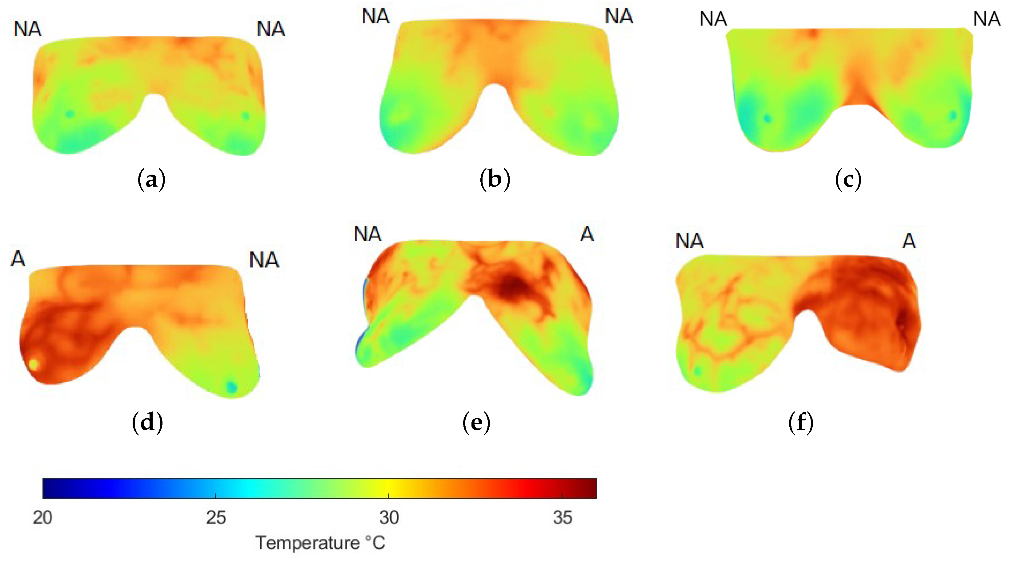
Figure 5 shows some samples of thermograms from the control group where the CT classifier, with the best performance according to the previous analysis, detected no anomalies (NAs) and where a high degree of symmetry in temperature distribution was observed. Although some subtle changes are perceived, they do not represent a significant difference. Nevertheless, in the samples identified with anomalies (As), the difference in thermal distribution is higher with increased temperatures in the breast with cancer confirmed by biopsy. Additionally, changes in vascularization have been identified in surrounding areas where the tumor develops as a result of the angiogenesis process (Figure 5d–f).
To complement these observations, Table 5 reports selected feature values for a control and a cancer case. Figure 5a illustrates a control example in which both breasts were labeled NA. Although their mean temperature values are similar, the right breast exhibits a broader, warmer region with slight vascularization, resulting in higher entropy. This localized change also produces noticeable differences in minimum and maximum values compared with the left breast, while correlation decreases. However, homogeneity and contrast remain close across both sides, as each breast exhibits relatively regular inner regions. These findings suggest that, even in NA cases from the same subject, the features can capture subtle variations not apparent to visual inspection.
In contrast, Figure 5d corresponds to a subject with cancer confirmed in the left breast, while the right breast was labeled as healthy. Here, mean, minimum, and maximum temperatures are all higher than in the control example. More evident vascularization is also observed in the right breast, reflected in reduced homogeneity. Because elevated temperatures extend across large areas in both breasts, correlation values remain high. Entropy and contrast also increase, with the latter showing greater sensitivity to thermal changes. Altogether, these characteristics enabled the CL classifier to discriminate between normal and abnormal patterns in thermal images effectively.
These labels were aligned with the annotations provided by the experts in the database, thereby validating the classification accuracy.

4. Discussion

Some works have addressed this task under diverse approaches. Sathish et al. [41] initially selected 144 spectral features for thermography classification, achieving an accuracy of 87% with the Bagged Trees (BTs) classifier and 5-fold cross-validation. Subsequently, feature reduction and selection techniques were applied, reducing the number of features to 33. This optimization improved the classification accuracy to 93% when using Ensemble Bagged Trees. Similarly, Lennox et al. [42] employed a dataset of 60 thermograms and 19 selected features, achieving a maximum accuracy of 90% with the Random Forest classifier. This study utilized a Leave-One-Out Cross-Validation scheme, highlighting its utility in evaluating model robustness and reliability. Kumar et al. [43] used a larger dataset of 200 thermograms and 20 selected features, achieving a maximum accuracy of 92.70% with the DT classifier. Other works have considered avoiding redundancy in exhaustive feature extraction. In [44], several feature selection strategies were applied, obtaining a reduced description down to six features and performing classification using an Artificial Neural Network (ANN). Additionally, this description was tested over thermograms from different groups considering ages between 20 and 80, obtaining accuracy ranging between 79.3 and 74.7%; the overall performance reached an accuracy of 88.57%. Recently, Mirasbekov et al. [45] analyzed a dataset of 364 thermograms (153 cancer, 211 healthy) using a CNN and Transfer Learning. The accuracy achieved was 90.93%.
The application of CNN and DL in thermography classification has been widely studied due to its potential advantages. However, its effectiveness depends on several critical factors. First, these models require large and diverse datasets to achieve robust training; otherwise, they are prone to overfitting and limited generalization [46]. This issue is particularly relevant in medical imaging, where data availability is often restricted. Indeed, some studies have reported that simpler ML models can outperform DL approaches in breast cancer detection, offering more reliable and practical results [47]. Consequently, the limitations of DL—especially its sensitivity to dataset size and variability—may hinder its performance in real-world applications or when new datasets are introduced. Feature selection significantly influences classification outcomes, and studies indicate that more cautious selection methods can yield better accuracy than exhaustive extraction techniques [48,49,50]. The CT classifier yielded the best results with the proposed description, reaching an accuracy of 91.97%.
Related works shown in Table 6 reveal that the number of features employed by researchers vary significantly. In the classification of breast thermographies, feature selection has been considered a relevant step to reduce computational costs and redundant features, helping to avoid overfitting and improve performance. In the present study, ML models were selected as a viable option due to the limitations associated with DL approaches, particularly the need for large datasets. This decision was validated by the results obtained, which demonstrated competitive performance compared with previous studies. A key advantage of this approach was the use of a reduced set of features, which not only optimized the model’s performance but also underscored the potential of ML techniques in achieving robust outcomes with limited data. By focusing on proper feature selection and modeling, this study advanced the field by illustrating that effective and reliable classification can be achieved without the extensive computational and data requirements of DL. This reinforces the critical importance of tailoring the model selection process to align with the specific characteristics and constraints of the problem being addressed and highlights the effectiveness of streamlined approaches in delivering reliable and efficient solutions in thermographic image classification.
The implementation of thermography has been extensively evaluated by various authors, who have obtained results supporting its potential as an effective complementary tool for detecting anomalies associated with breast cancer. This technique stands out for its ability to provide relevant information not observable through conventional methods. The results obtained in this work have proved that it is possible to achieve high-performance results with a lightweight description. This description was able to distinguish among the samples that presented significant thermal differences, which is consistent with the expert classification of healthy/cancer. Moreover, the applied tests provide a more reliable and rigorous framework for validating results, ensuring that the reported performance accurately reflects the true model behavior rather than random variation. The obtained CIs showed that the proposed description remains highly stable despite the used classifier.
Despite these promising results, some limitations remain. The results were obtained on a dataset of limited size. A larger and different dataset is required for external validation and generalization. Also, the analysis is limited to a binary identification of healthy and cancer samples. Not only a larger dataset but also a more precise labeling that includes intermediate classes or a possible association with the standard BI-RADS grades is required. Therefore, a continuous improvement in the research of thermal images for detecting risk cancer is necessary.

5. Conclusions

Through studies analyzing the functionality and utility of clinical thermography, it has been demonstrated that this is a valuable complementary tool for evaluating anomalies related to breast cancer, as skin temperature has been established as a sign of disease. Furthermore, these thermal changes are often imperceptible to the naked eye. However, some of these thermal changes may be so subtle that they are not visible to the naked eye, which underscores the need for automated models capable of precise analysis and accurate classification of thermographic features.
In this study, ML models were employed, demonstrating competitive accuracy in the individual analysis of each breast. This was achieved through feature selection and testing several classifiers, a critical aspect consistent with previous reports, as proper feature selection leads to better classification results. The results showed that an accuracy of 91.97% can be achieved, outperforming previous studies and competing with sophisticated current approaches, while avoiding exhaustive feature extraction. Moreover, a brief description enables the correlation of relevant features with clinical observations, thereby increasing the interpretability of the description. The proposed approach not only aligned with expert classifications but also proved to be stable across classifiers, as confirmed through statistical testing and the analysis of confidence intervals. This study demonstrated that selected ML models can accurately classify breast thermograms, offering a short description that can be used to complement standard diagnostic methods.
As future work, this hypothesis will be addressed along with the exploration of hybrid models to improve results. Moreover, expanding the current database, automating the masks generation, and incorporating new features from other domains is a worthwhile area for future investigation.

Author Contributions

Conceptualization and methodology, A.P.R.-C. and H.P.-B.; validation, H.P.-B. and J.J.R.-M.; investigation, A.P.R.-C., H.P.-B. and F.J.R.-C.; resources, J.J.R.-M. and J.M.R.-C.; writing—original draft preparation, A.P.R.-C.; writing—review and editing, H.P.-B. and J.J.R.-M.; supervision, H.P.-B. All authors have read and agreed to the published version of the manuscript.

Funding

This research received no external funding.

Institutional Review Board Statement

Ethical review and approval were waived for this study due to the data used were obtained from the public databases.

Informed Consent Statement

Patient consent was waived due to the data used were obtained from the public databases.

Data Availability Statement

The dataset analyzed in this study belongs to the DMR—Database For Mastology Research at https://visual.ic.uff.br/dmi/(accessed on 8 October 2025), which was previously reported in [19].

Acknowledgments

The author Ana P. Romero-Carmona thanks SECIHTI (Mexico) for the scholarship awarded for this work.

Conflicts of Interest

The authors declare no conflicts of interest.

References

  1. Zarate, C.M.; Jankowski, M.R.; Sullivan, S.E. Effect of Promensil on T47D Breast Cancer Cells with Respect to Estrogen Receptors Alpha and Beta; Worcester Polytechnic Institute: Worcester, MA, USA, 2020. [Google Scholar]
  2. Sung, H.; Ferlay, J.; Siegel, R.L.; Laversanne, M.; Soerjomataram, I.; Jemal, A.; Bray, F. Global cancer statistics 2020: GLOBOCAN estimates of incidence and mortality worldwide for 36 cancers in 185 countries. CA Cancer J. Clin. 2021, 71, 209–249. [Google Scholar] [CrossRef]
  3. Morton Cuthrell, K.; Tzenios, N. Breast Cancer: Updated and Deep Insights. Int. Res. J. Oncol. 2023, 6, 104–118. [Google Scholar]
  4. Ginsburg, O.; Yip, C.H.; Brooks, A.; Cabanes, A.; Caleffi, M.; Dunstan Yataco, J.A.; Gyawali, B.; McCormack, V.; McLaughlin de Anderson, M.; Mehrotra, R.; et al. Breast cancer early detection: A phased approach to implementation. Cancer 2020, 126, 2379–2393. [Google Scholar] [CrossRef]
  5. Kiymet, S.; Aslankaya, M.Y.; Taskiran, M.; Bolat, B. Breast cancer detection from thermography based on deep neural networks. In Proceedings of the 2019 Innovations in Intelligent Systems and Applications Conference (ASYU), Izmir, Turkey, 31 October–2 November 2019; IEEE: Piscataway, NJ, USA, 2019; pp. 1–5. [Google Scholar]
  6. Liu, Q.; Li, M.; Wang, W.; Jin, S.; Piao, H.; Jiang, Y.; Li, N.; Yao, H. Infrared thermography in clinical practice: A literature review. Eur. J. Med. Res. 2025, 30, 33. [Google Scholar] [CrossRef] [PubMed]
  7. Gonzalez-Hernandez, J.L.; Recinella, A.N.; Kandlikar, S.G.; Dabydeen, D.; Medeiros, L.; Phatak, P. Technology, application and potential of dynamic breast thermography for the detection of breast cancer. Int. J. Heat Mass Transf. 2019, 131, 558–573. [Google Scholar] [CrossRef]
  8. Singh, D.; Singh, A.K. Role of image thermography in early breast cancer detection-Past, present and future. Comput. Methods Programs Biomed. 2020, 183, 105074. [Google Scholar] [CrossRef]
  9. Cook, K.M.; Figg, W.D. Angiogenesis inhibitors: Current strategies and future prospects. CA Cancer J. Clin. 2010, 60, 222–243. [Google Scholar] [CrossRef] [PubMed]
  10. Spalding, S.; Kwoh, C.; Boudreau, R.; Enama, J.; Lunich, J.; Huber, D.; Denes, L.; Hirsch, R. Three-dimensional and thermal surface imaging produces reliable measures of joint shape and temperature: A potential tool for quantifying arthritis. Arthritis Res. Ther. 2008, 10, 10. [Google Scholar] [CrossRef]
  11. Adam, M.; Ng, E.; Tan, J.; Heng, M.; Tong, J.; Acharya, U. Computer aided diagnosis of diabetic foot using infrared thermography: A review. Comput. Biol. Med. 2017, 91, 326–336. [Google Scholar] [CrossRef]
  12. Li, C.; Liu, Y. Detecting intersegmental plane in thoracoscopic segmentectomy using infrared thermography. Chin. Med. J. 2022, 135, 119–120. [Google Scholar] [CrossRef]
  13. Mambou, S.J.; Maresova, P.; Krejcar, O.; Selamat, A.; Kuca, K. Breast cancer detection using infrared thermal imaging and a deep learning model. Sensors 2018, 18, 2799. [Google Scholar] [CrossRef] [PubMed]
  14. Kesztyüs, D.; Bae, H.; Wilson, C.; Schön, M.; Kesztyüs, T. Non-invasive infrared thermography for screening, diagnosis and monitoring of skin cancer. J. Dtsch. Dermatol. Ges. 2024, 23, 7–17. [Google Scholar] [CrossRef] [PubMed]
  15. Dong, F.; Tao, C.; Wu, J.; Su, Y.; Wang, Y.; Wang, Y.; Lyu, P. Detection of cervical lymph node metastasis from oral cavity cancer using a non-radiating, noninvasive digital infrared thermal imaging system. Sci. Rep. 2018, 8, 7219. [Google Scholar] [CrossRef]
  16. Javaid, M.; Haleem, A.; Singh, R.P.; Ahmed, M. Computer vision to enhance healthcare domain: An overview of features, implementation, and opportunities. Intell. Pharm. 2024, 2, 792–803. [Google Scholar] [CrossRef]
  17. Kaushik, R.; Sivaselvan, B.; Kamakoti, V. Clinical Thermography for Breast Cancer Screening: A Systematic Review on Image Acquisition, Segmentation, and Classification. IETE Tech. Rev. 2024, 41, 238–260. [Google Scholar] [CrossRef]
  18. Mashekova, A.; Zhao, Y.; Ng, E.Y.; Zarikas, V.; Fok, S.C.; Mukhmetov, O. Early detection of the breast cancer using infrared technology—A comprehensive review. Therm. Sci. Eng. Prog. 2022, 27, 101142. [Google Scholar] [CrossRef]
  19. Silva, L.; Saade, D.; Sequeiros, G.; Silva, A.; Paiva, A.; Bravo, R.; Conci, A. A new database for breast research with infrared image. J. Med. Imaging Health Inform. 2014, 4, 92–100. [Google Scholar] [CrossRef]
  20. Gonzalez, R.C.; Woods, R.E. Digital Image Processing, 4th ed.; Pearson: Prentice Hall, NJ, USA, 2017; ISBN 9780133356724. [Google Scholar]
  21. Motoyoshi, I.; Nishida, S.; Sharan, L.; Adelson, E.H. Image statistics and the perception of surface qualities. Nature 2007, 447, 206–209. [Google Scholar] [CrossRef]
  22. Dey, S. Hands-On Image Processing with Python: Expert Techniques for Advanced Image Analysis and Effective Interpretation of Image Data; Packt Publishing Ltd.: Birmingham, UK, 2018. [Google Scholar]
  23. Singh, H.; Sharma, V.; Singh, D. Comparative analysis of proficiencies of various textures and geometric features in breast mass classification using k-nearest neighbor. Vis. Comput. Ind. Biomed. Art 2022, 5, 3. [Google Scholar] [CrossRef]
  24. Rindskopf, D.; Shiyko, M. Measures of Dispersion, Skewness and Kurtosis. In International Encyclopedia of Education, 3rd ed.; Peterson, P., Baker, E., McGaw, B., Eds.; Elsevier: Oxford, UK, 2010; pp. 267–273. [Google Scholar] [CrossRef]
  25. Humeau-Heurtier, A. Texture Feature Extraction Methods: A Survey. IEEE Access 2019, 7, 8975–9000. [Google Scholar] [CrossRef]
  26. Mishra, P.; Singh, U.; Pandey, C.M.; Mishra, P.; Pandey, G. Application of student’s t-test, analysis of variance, and covariance. Ann. Card. Anaesth. 2019, 22, 407–411. [Google Scholar] [CrossRef]
  27. King, A.P.; Eckersley, R. Statistics for Biomedical Engineers and Scientists: How to Visualize and Analyze Data; Academic Press: Cambridge, MA, USA, 2019. [Google Scholar]
  28. Mahesh, T.R.; Vinoth Kumar, V.; Dhilip Kumar, V.; Geman, O.; Margala, M.; Guduri, M. The stratified K-folds cross-validation and class-balancing methods with high-performance ensemble classifiers for breast cancer classification. Healthc. Anal. 2023, 4, 100247. [Google Scholar] [CrossRef]
  29. Goodfellow, I.; Bengio, Y.; Courville, A.; Bengio, Y. Deep Learning; MIT Press Cambridge: Cambridge, MA, USA, 2016; Volume 1. [Google Scholar]
  30. Domingos, P. A few useful things to know about machine learning. Commun. ACM 2012, 55, 78–87. [Google Scholar] [CrossRef]
  31. Wang, P.; Fan, E.; Wang, P. Comparative analysis of image classification algorithms based on traditional machine learning and deep learning. Pattern Recognit. Lett. 2021, 141, 61–67. [Google Scholar] [CrossRef]
  32. Hwang, J.H.; Seo, J.W.; Kim, J.H.; Park, S.; Kim, Y.J.; Kim, K.G. Comparison between deep learning and conventional machine learning in classifying iliofemoral deep venous thrombosis upon CT venography. Diagnostics 2022, 12, 274. [Google Scholar] [CrossRef] [PubMed]
  33. Awad, M.; Khanna, R. Support vector machines for classification. In Efficient Learning Machines: Theories, Concepts, and Applications for Engineers and System Designers; Springer Nature: Berlin/Heidelberg, Germany, 2015; pp. 39–66. [Google Scholar]
  34. Sperandei, S. Understanding logistic regression analysis. Biochem. Medica 2014, 24, 12–18. [Google Scholar] [CrossRef]
  35. Agresti, A. An Introduction to Categorical Data Analysis, 1st ed.; Wiley Series in Probability and Statistics; John Wiley & Sons, Inc.: Hoboken, NJ, USA, 2006. [Google Scholar] [CrossRef]
  36. Subbarao, M.V.; Samundiswary, P. Automatic modulation recognition in cognitive radio receivers using multi-order cumulants and decision trees. Int. J. Rec. Technol. Eng. 2018, 7, 61–69. [Google Scholar]
  37. Mokhtar, S.; Yusof, Z.; Sapiri, H. Confidence Intervals by Bootstrapping Approach: A Significance Review. Malays. J. Fundam. Appl. Sci. 2023, 19, 30–42. [Google Scholar] [CrossRef]
  38. Gitto, S.; Annovazzi, A.; Nulle, K.; Interlenghi, M.; Salvatore, C.; Anelli, V.; Baldi, J.; Messina, C.; Albano, D.; Di Luca, F.; et al. X-rays radiomics-based machine learning classification of atypical cartilaginous tumour and high-grade chondrosarcoma of long bones. eBioMedicine 2024, 101, 105018. [Google Scholar] [CrossRef] [PubMed]
  39. Foody, G.M. Thematic Map Comparison. Photogramm. Eng. Remote Sens. 2004, 70, 627–633. [Google Scholar] [CrossRef]
  40. Yan, L. Confidence interval estimation of the common mean of several gamma populations. PLoS ONE 2022, 17, e0269971. [Google Scholar] [CrossRef]
  41. Sathish, D.; Kamath, S. Detection of breast thermograms using ensemble classifiers. J. Telecommun. Electron. Comput. Eng. 2018, 10, 35–39. [Google Scholar]
  42. Lennox, N.; Haskins, B. Contrasting classifiers for the detection of breast cancer using thermographic images. In Proceedings of the 2nd International Conference on Intelligent and Innovative Computing Applications, New York, NY, USA, 24–25 September 2020. ICONIC ’20. [Google Scholar] [CrossRef]
  43. Aggarwal, A.K.; Alpana; Pandey, M. Machine Learning Approach for Breast Cancer Detection using Thermal Imaging. In Proceedings of the 2022 Second International Conference on Next Generation Intelligent Systems (ICNGIS), Kottayam, India, 29–31 July 2022; pp. 1–5. [Google Scholar] [CrossRef]
  44. Gupta, K.K.; Vijay, R.; Pahadiya, P.; Saxena, S.; Gupta, M. Novel feature selection using machine learning algorithm for breast cancer screening of thermography images. Wirel. Pers. Commun. 2023, 131, 1929–1956. [Google Scholar] [CrossRef]
  45. Mirasbekov, Y.; Aidossov, N.; Mashekova, A.; Zarikas, V.; Zhao, Y.; Ng, E.Y.K.; Midlenko, A. Fully interpretable deep learning model using IR thermal images for possible breast cancer cases. Biomimetics 2024, 9, 609. [Google Scholar] [CrossRef]
  46. Loukil, Z.; Mirza, Q.K.A.; Sayers, W.; Awan, I. A deep learning based scalable and adaptive feature extraction framework for medical images. Inf. Syst. Front. 2024, 26, 1279–1305. [Google Scholar] [CrossRef]
  47. Karthiga, R.; Narasimhan, K.; Thanikaiselvan, V.; Hemalatha, M.; Amirtharajan, R. Review of AI & XAI-based breast cancer diagnosis methods using various imaging modalities. Multimed. Tools Appl. 2024, 84, 2209–2260. [Google Scholar] [CrossRef]
  48. Kabir, M.H.; Akhtar, N.I.; Tasnim, N.; Miah, A.S.M.; Lee, H.S.; Jang, S.W.; Shin, J. Exploring Feature Selection and Classification Techniques to Improve the Performance of an Electroencephalography-Based Motor Imagery Brain–Computer Interface System. Sensors 2024, 24, 4989. [Google Scholar] [CrossRef] [PubMed]
  49. Ahmed, B.; Naqvi, S.R.; Akram, T.; Peng, L.; Almarshad, F. A Hybrid Deep Learning-ViT Model and A Meta-Heuristic Feature Selection Algorithm for Efficient Remote Sensing Image Classification. Int. J. Comput. Intell. Syst. 2025, 18, 122. [Google Scholar] [CrossRef]
  50. Zhang, W.; Guo, Y.; Jin, Q. Radiomics and its feature selection: A review. Symmetry 2023, 15, 1834. [Google Scholar] [CrossRef]
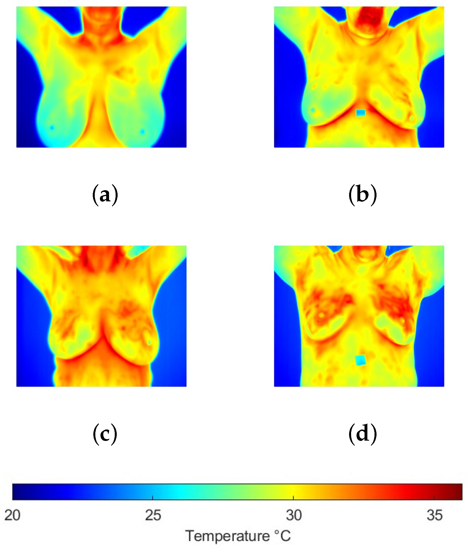
Figure 1. Breast thermograms samples from the (a,b) control and (c,d) cancer groups, where it is observed that increased temperatures are present in the second group.
Jimaging 11 00358 g001
Figure 2. (a) Breast thermogram and (b) its corresponding binary mask.
Jimaging 11 00358 g002
Figure 3. Illustration of the stratified 5-fold cross-validation procedure, where each fold is used once as the test set (yellow) while the remaining folds (blue) are used for training.
Jimaging 11 00358 g003
Figure 4. Different conditions of temperature among breasts from the same subject.
Jimaging 11 00358 g004
Figure 5. Examples of the breast region extraction in thermograms (ac) of the control and (df) cancer groups. Labels above each breast indicate whether no anomalies (NA) or anomalies (A) were detected using the CT classifier, matching the expert’s label.
Jimaging 11 00358 g005
Table 1. Student’s t-test p-value of the analyzed features.
Featurep-Value
Homogeneity0.0295
Contrast0.0000
Correlation0.0009
E 0.1408
μ 0.0000
σ 0.4762
σ 2 0.9625
γ 0.3051
k0.3477
H0.0018
Min0.0018
Max0.0000
C V 0.4189
Table 2. Classification results of breast thermograms considering a five-fold cross-validation.
MetricsL-SVMQ-SVMLRCT
Accuracy84.93 % ± 0.02390.99 % ± 0.01984.93 % ± 0.02091.97 % ± 0.015
Precision83.43 % ± 0.02988.41 % ± 0.01185.04 % ± 0.01990.79 % ± 0.025
Recall87.32 % ± 0.04294.37 % ± 0.04284.79 % ± 0.03493.52 % ± 0.027
F1-score85.27 % ± 0.02491.256 % ± 0.02084.89 % ± 0.02292.09 % ± 0.014
Table 3. Mean performance metrics evaluation with their 95% bootstrap CIs for breast thermogram classification.
MetricsL-SVMQ-SVMLRCT
Accuracy84.92 [82.25–87.46]90.95 [88.87–93.10]84.96 [82.39–87.61]91.97 [90.00–93.94]
Precision83.28 [80.15–86.38]88.41 [85.53–91.20]85.10 [82.07–88.12]90.74 [88.14–93.34]
Recall87.31 [83.94–90.70]94.36 [91.83–96.62]84.85 [81.13–88.45]93.50 [90.70–95.77]
Specificity82.60 [78.59–86.48]87.62 [84.23–90.99]85.12 [81.41–88.73]90.43 [87.04–93.52]
F1-score85.28 [82.58–87.74]91.30 [89.18–93.19]84.91 [82.16–87.61]92.08 [90.16–93.98]
Table 4. Pairwise comparison of classifier performance using McNemar’s test.
PairDifference95% CIp-Value
L-SVM vs. Q-SVM−0.10 [ 0.72 , 0.57 ] 1.00
L-SVM vs. LR0.60 [ 0.69 , 0.99 ] 1.00
L-SVM vs. CT0.07 [ 0.62 , 0.67 ] 1.00
Q-SVM vs. LR0.33 [ 0.42 , 0.92 ] 1.00
Q-SVM vs. CT0.25 [ 0.73 , 0.95 ] 1.00
LR vs. CT−0.16 [ 0.74 , 0.51 ] 1.00
Table 5. Feature description of thermograms in Figure 5.
NameLabelMeanEntropyMinMaxHomogeneityContrastCorrelation
Figure 5a-LNA27.50980.696923.4631.860.62864.00950.9922
Figure 5a-RNA27.67460.734621.8432.590.64333.92720.9912
Figure 5d-LA31.59110.713023.1333.570.66394.40110.9896
Figure 5d-RNA29.18740.750622.7533.630.70483.44180.9950
Table 6. Summary of studies on the use of thermography and the evaluation of AI techniques for the early detection of breast cancer.
WorkClassification ModelSamplesFeaturesBalanced ClassesAccuracy
Sathish et al. [41]
(2018)
BT
Ensemble BT
-33-87.00%
71.00%
Lennox et al. [42]
(2021)
Random Forest
ANN
SVM RBF
6019Yes90.00%
88.33%
88.33%
Kumar et al. [43]
(2022)
DT
KNN
LDA
20020Yes92.70%
91.00%
84.80%
Gupta et al. [44]
(2023)
ANN2786-88.57%
Mirasbekov et al. [45]
(2024)
CNN
Transfer Learning
364-Yes90.93%
ProposedCT1417Yes91.97%
Disclaimer/Publisher’s Note: The statements, opinions and data contained in all publications are solely those of the individual author(s) and contributor(s) and not of MDPI and/or the editor(s). MDPI and/or the editor(s) disclaim responsibility for any injury to people or property resulting from any ideas, methods, instructions or products referred to in the content.