

A Systematic Literature Review of Waste Identification in Automatic Separation Systems

 , and
, and
Abstract
:
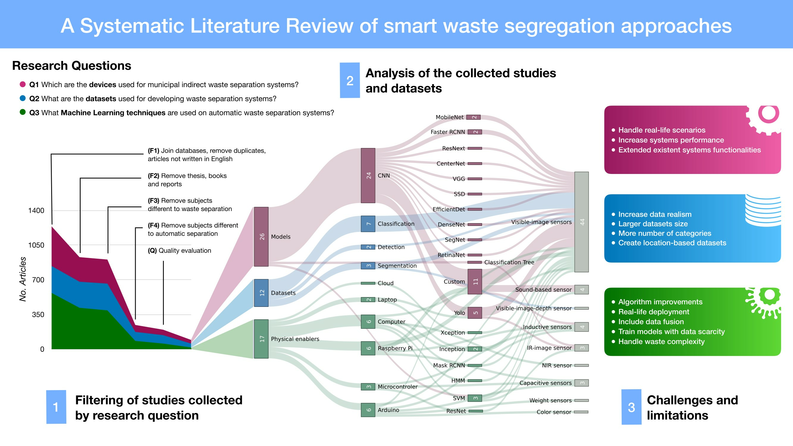
1. Introduction
- The identification of indirect segregation machines sensors, processing devices, complementary functionalities, and their implementation context (Section 3.1).
- A characterization of the datasets used by waste separation systems with sorting categories, environments for collecting the observations, and geographical locations, among other elements (Section 3.2).
- The identification of public datasets for developing ML models for waste identification (Section 3.2).
- The identification of ML algorithms used for waste identification, their model architecture, and feature extractors, including analysis of the performance metrics used by the models and the objects and materials identified (Section 3.3).
- The compilation of ML algorithms’ benchmark on public datasets for waste identification (Section 3.3).
- A holistic view of relationships between hardware, ML algorithms, and datasets (Section 3.4).
- The definition of challenges and limitations of waste identification systems (Section 4).
2. Methodology
2.1. Planning the Review
2.1.1. Related Work
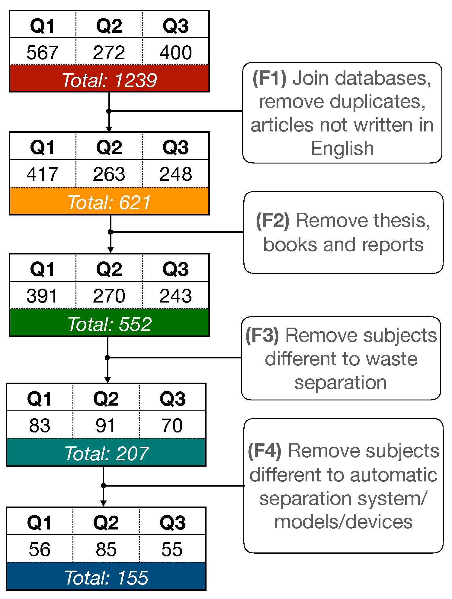
2.1.2. Search Protocol
2.2. Conducting the Review
3. Results
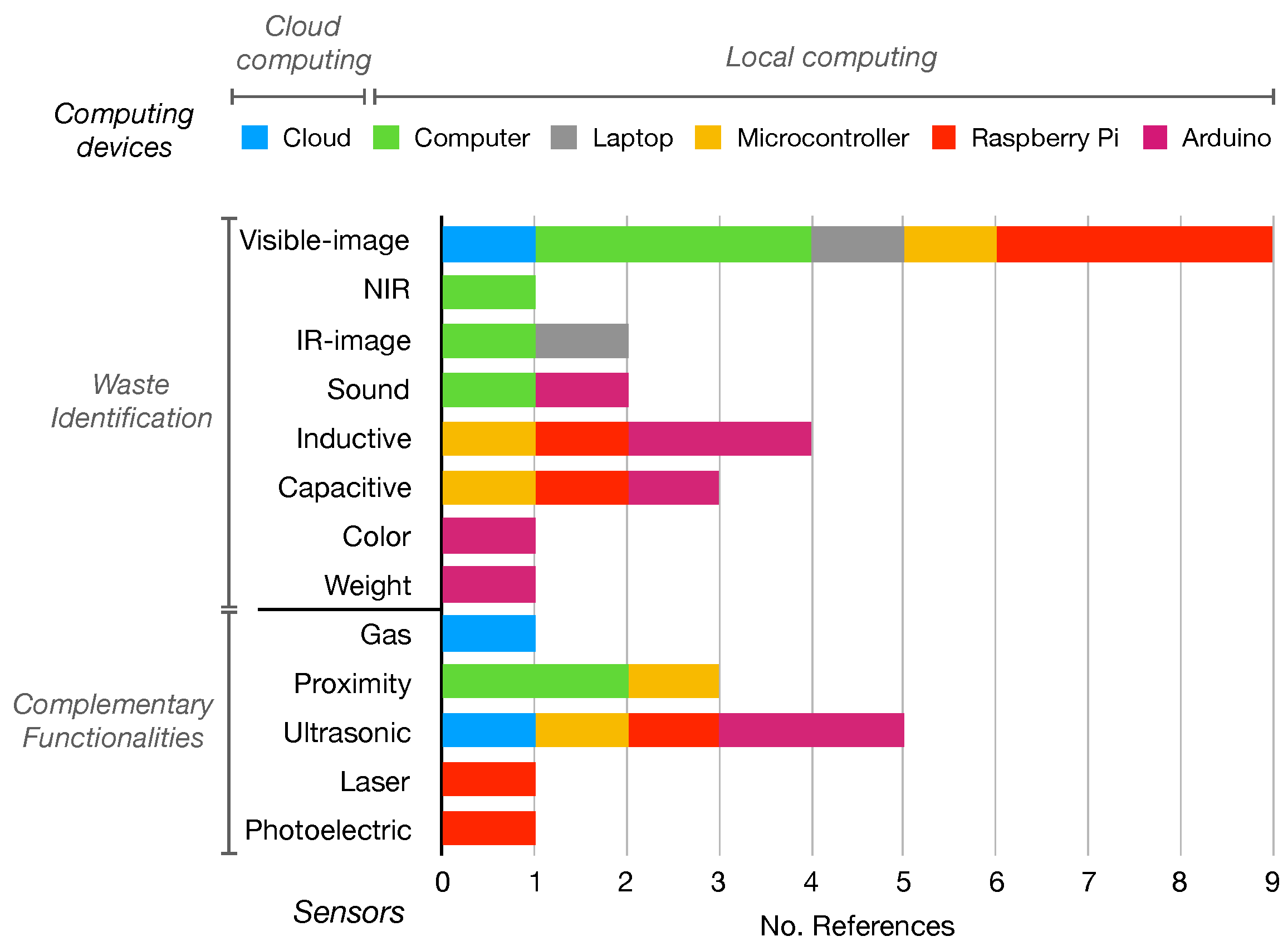
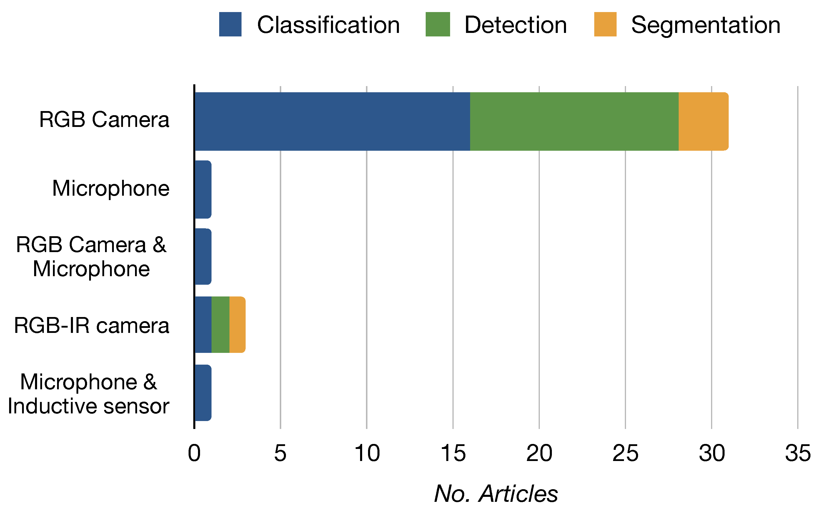
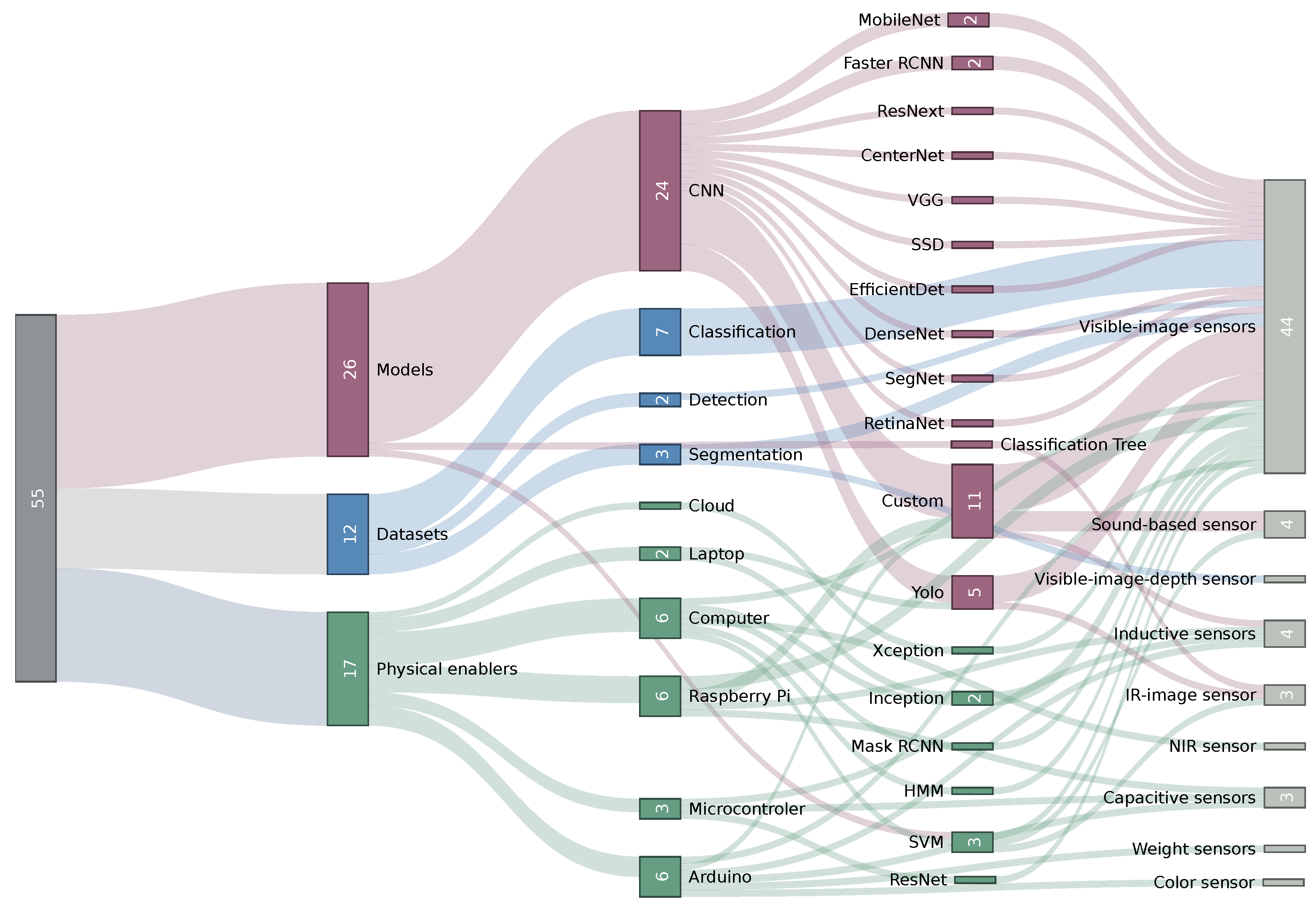
3.1. Physical Enablers
- (i)
- Full automation:system automatically seeks, classifies, and separates waste. A robot using IR cameras, proximity sensors, and robotic arms identifies objects on the ground to this end [34].
- (ii)
- Moderate autonomy: The system classifies and separates the waste. Nevertheless, the feeding is performed by the user. Two different layouts can be observed:
- (a)
- Continuous feeding: A conveyor belt ensures the waste is always sensed in the same spot. Sensing is performed using visible-image-based sensors (most common) [9,35,36,37,38,39], inductive and capacity sensors [8], near-infrared (NIR) sensors [35], and weight sensors [40]. Subsequently, the waste is classified and segregated towards the corresponding container using sorting arms [9,35], pneumatic actuators [36], servomotors [8,38,40], or falling on an inclined platform [39]. This is the most popular system layout, proposed in 8 of 17 articles.
- (b)
- Manual feeding: The user deposits the pieces of waste, one at a time, to be sensed by the device. Visible-image-based [6,7,41] and sound-based sensors [12], as well as inductive and capacitive sensors [42], are used for sensing. Afterwards, a gravity-based mechanism is used to perform the separation.
- (iii)
- Low autonomy: The user is responsible for the feeding and separation of the waste. The system identifies the waste and guides the user to deposit it in the correct container by opening the corresponding lid to indicate where to deposit it [10,43]. Waste identification is performed with image classification [10], radio-frequency identification (RFID) [43], or the sound generated by the trash bags [44].
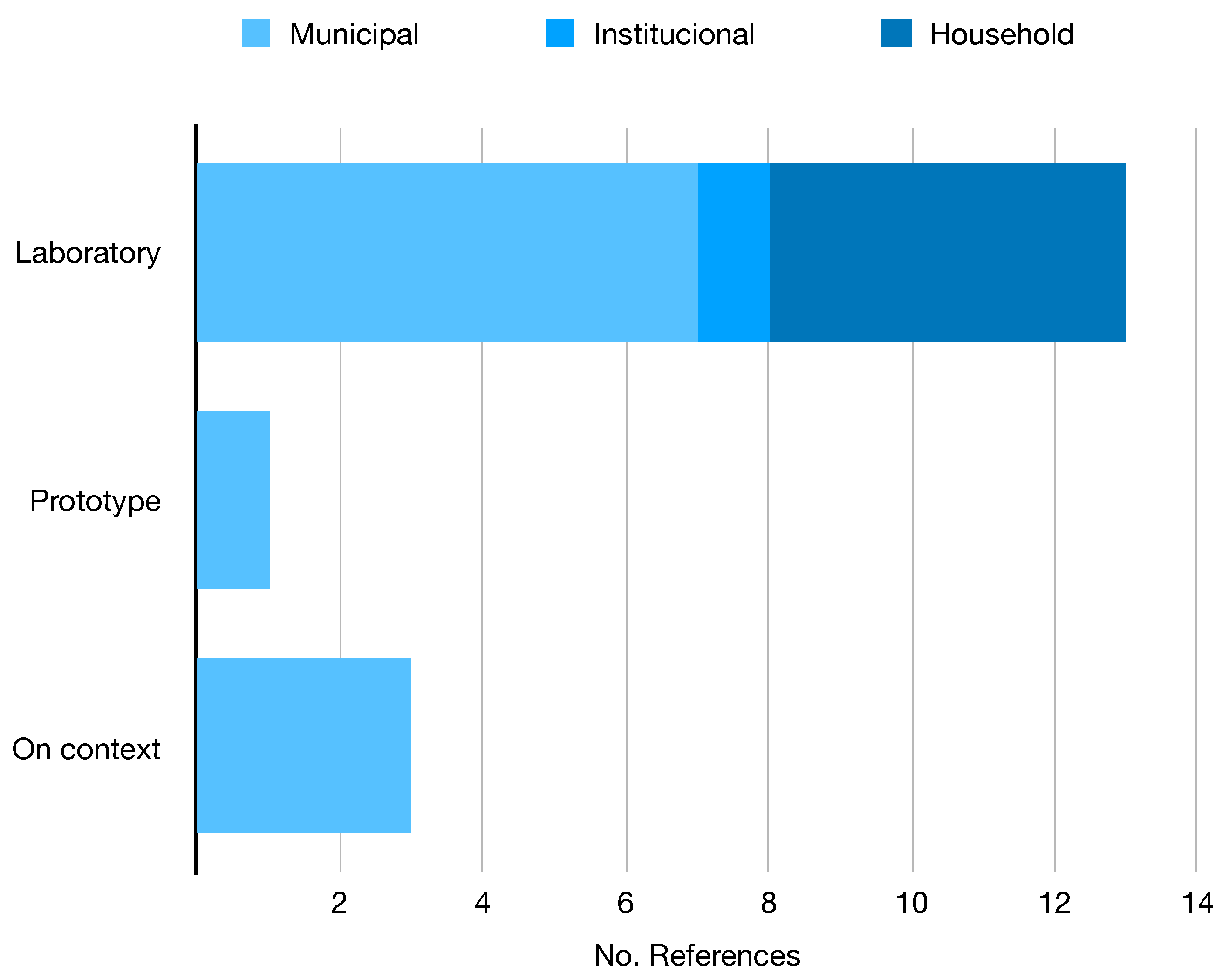
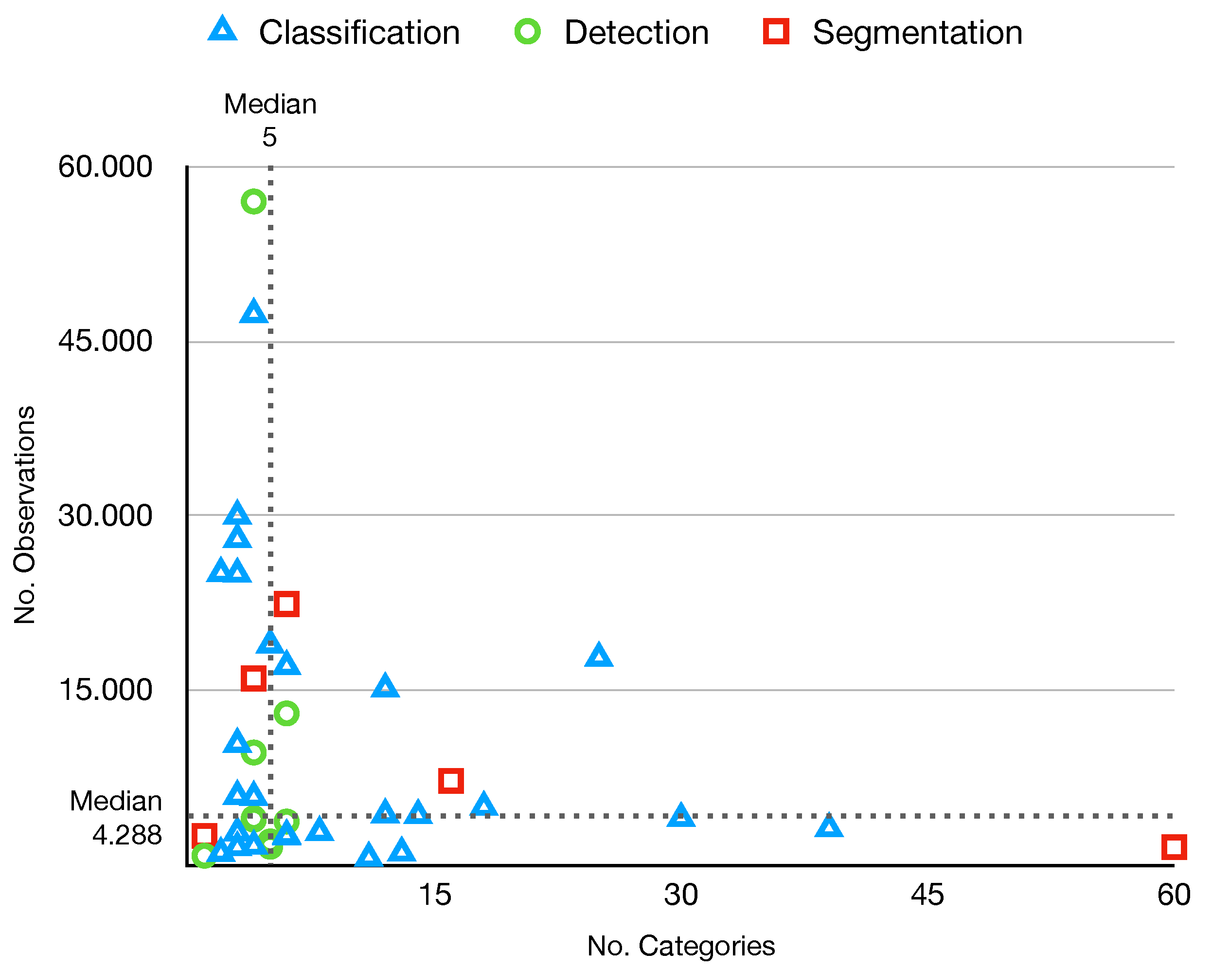
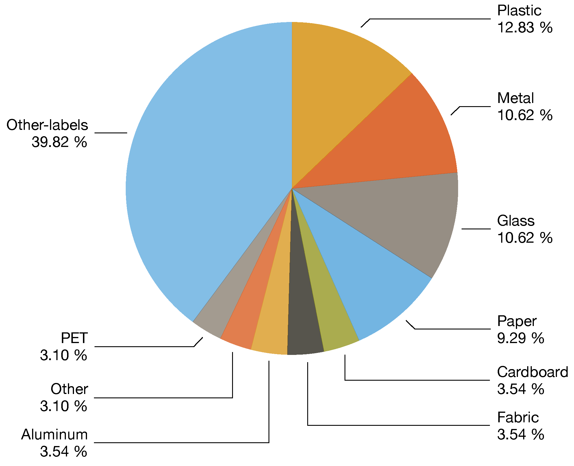
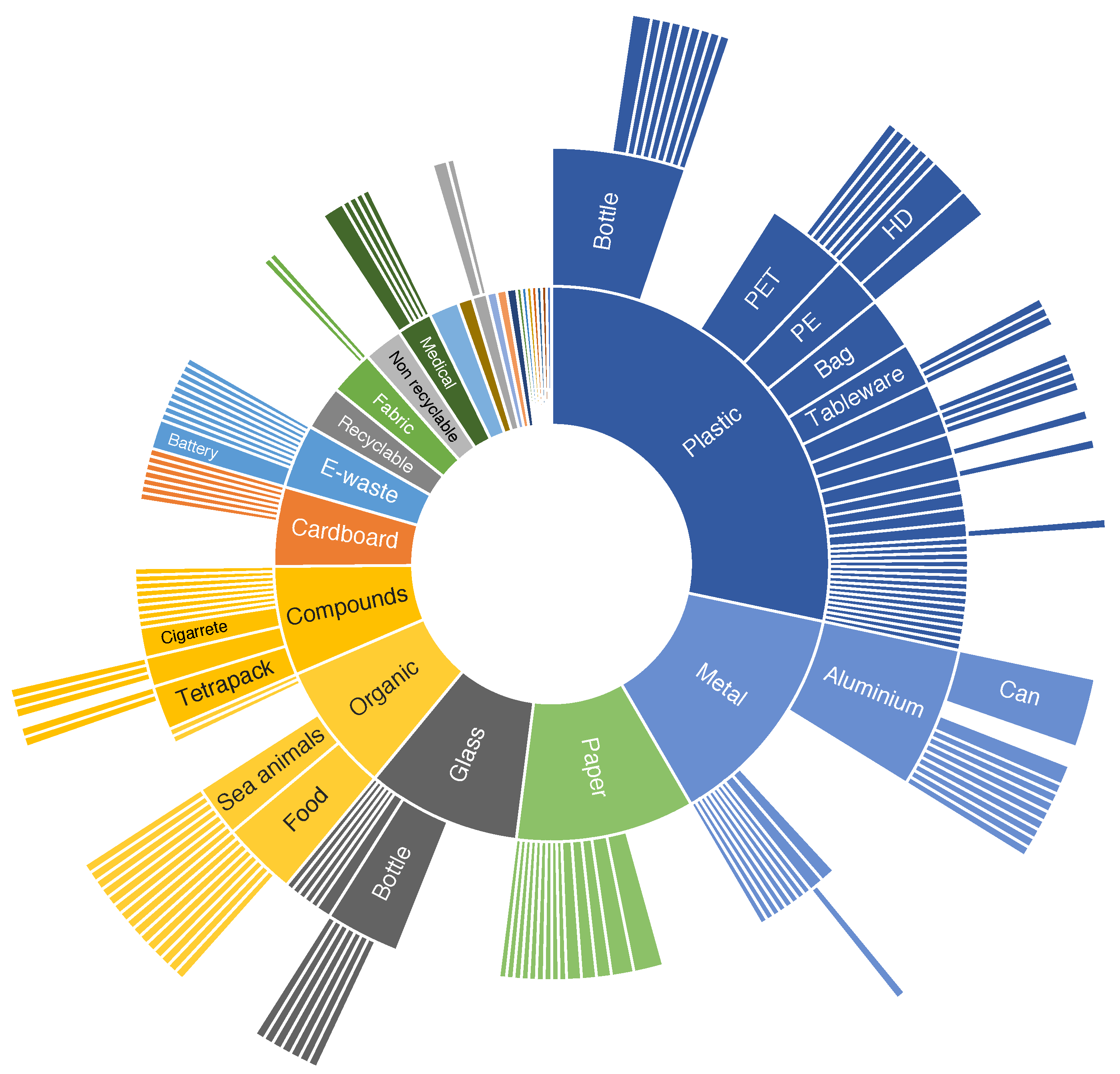
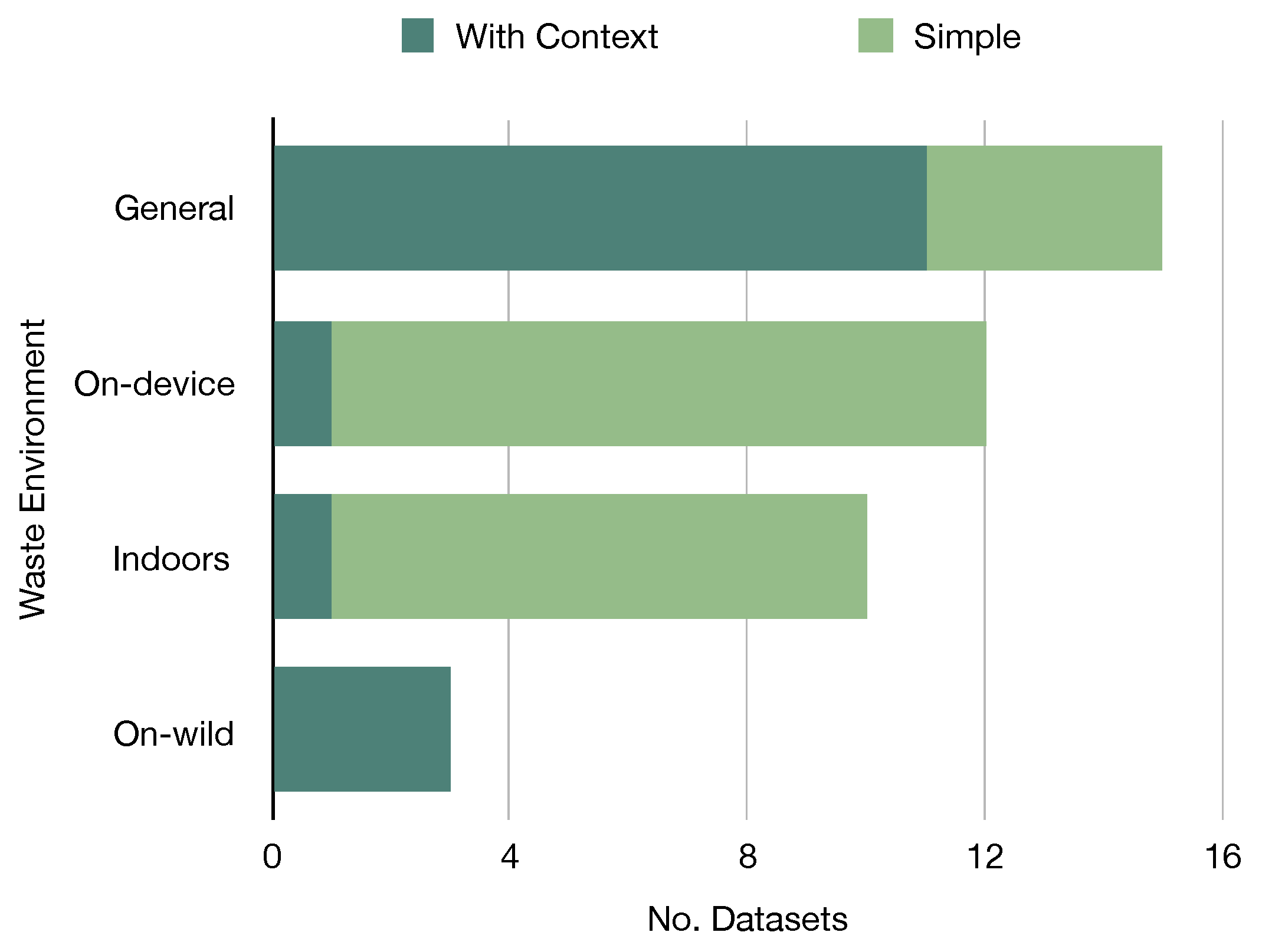
3.2. Datasets

| Year | Categories | Context | Studies | Size | Annotation | Location | Dist. | Ref |
|---|---|---|---|---|---|---|---|---|
| 2021 | 5–39 | On-device | [6] | 3126 | Classf | Italy | Baln | [6] |
| 2017 | 6 | General | [11,17,38,47,48,49,51,52,53,54] | 2527 | Classf | - | Unbl | [16] |
| 2021 | 3 | On-device | [55] | 10,391 | Classf | - | Baln | [55] |
| 2019 | 6 | Indoors | [56] | 2437 | Classf | - | Unbl | [57] |
| 2019 | 3 | General | [58] | 2751 | Classf | Mixed | Unbl | [58] |
| 2020 | 3 | Municipal | [59] | 25,000 | Classf | - | Unbl | [60] |
| 2018 | 8–30 | General | [15,61] | 4000 | Classf | Poland | Unbl | [15] |
| 2019 | 2 | General | [17] | 25,077 | Classf | - | Unbl | [62] |
| 2020 | 3 | General | - | 27,982 | Classf | - | Unbl | [60] |
| 2022 | 7–25 | - | - | 17,785 | Classf | - | Unbl | [14] |
| 2021 | 12 | General | - | 15,150 | Classf | - | Unbl | [63] |
| 2021 | 3–18 | Indoors | - | 4960 | Classf | - | Baln | [64] |
| 2021 | 4 | General | [9] | 16,000 | Segm | Greece | Baln | [9] |
| 2020 | 28–60 | On-wild | [18,37,65,66] | 1500 | Segm | - | Unbl | [18] |
| 2020 | 22–16 | Underwater | [67] | 7212 | Segm | - | Unbl | [67] |
| 2020 | 1 | Indoors | [68] | 2475 | Segm | - | - | [68] |
| 2019 | 4–6 | On-device | [46] | 3,000 | Detec | Rusia | Unbl | [46] |
| 2021 | 1 | Aerial | [69] | 772 | Detec | - | - | [69] |
| 2021 | 4 | General | [17] | 57,000 | Detec | - | Unbl | [17] |
| 2020 | 4 | Indoors | - | 9640 | Detec | - | Unbl | [70] |
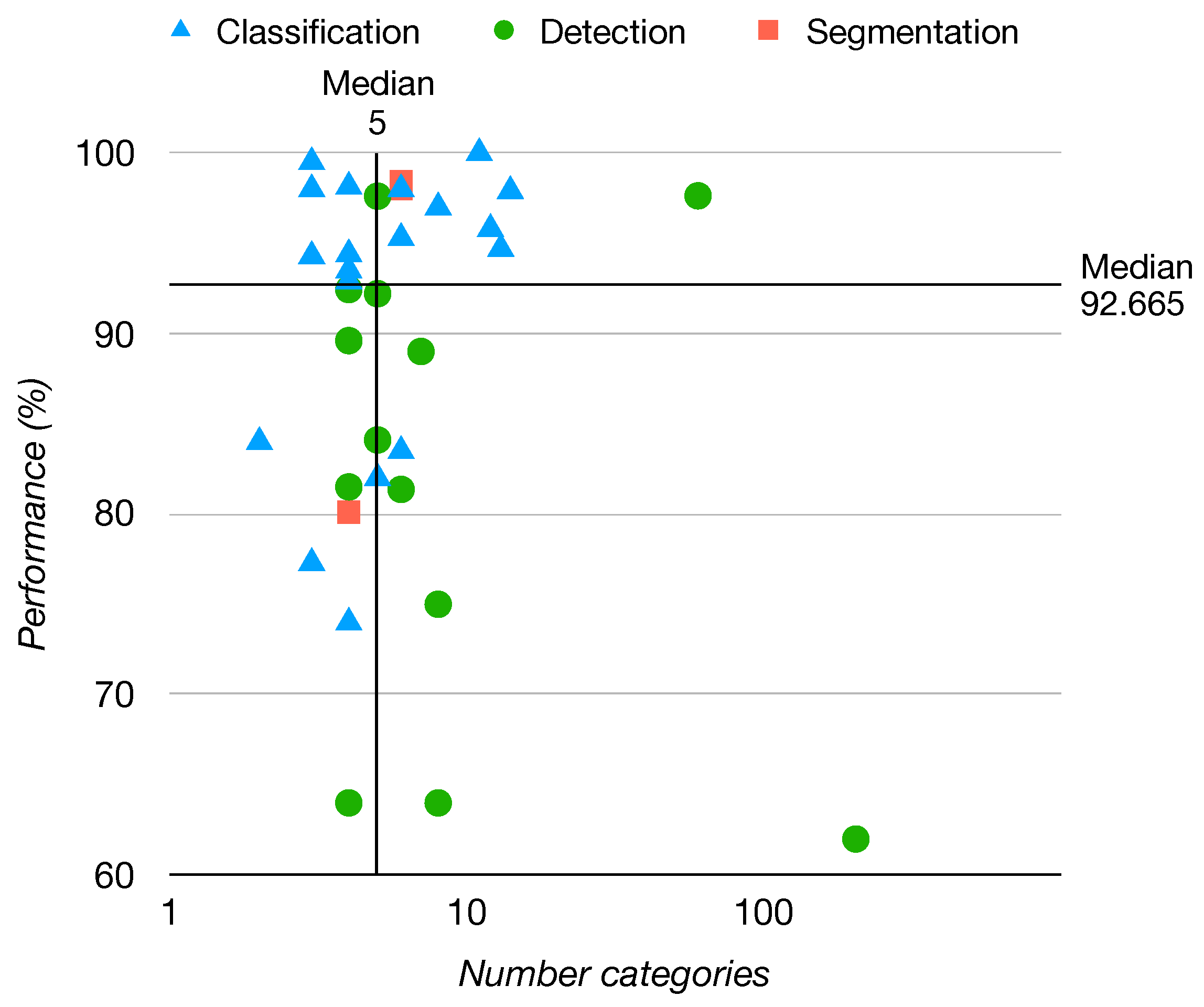
| Dataset | Study | Type | Architecture | Backbone | Extension | Acc. (%) | mAP (%) | IOU (%) |
|---|---|---|---|---|---|---|---|---|
| Trashnet | [51] | Classf | Resnext50 | Resnext | TL | 98 | - | - |
| [38] | Classf | Resnet34 | Resnet | TL | 95.3 | - | - | |
| [53] | Classf | Custom (CNN) | Resnext | TL | 94 | - | - | |
| [52] | Classf | Custom (CNN) | Googlenet, Resnet50, Mobilenet2 | - | 93.5 | - | - | |
| [54] | Classf | Custom (SVM) | Mobilenet2 | - | 83.5 | - | - | |
| [47] | Detec | SSD | MobileNet2 | TL | - | 97.6 | - | |
| [48] | Detec | Yolo4 | DarkNet53 | - | - | 89.6 | - | |
| [11] | Detec | Yolo3 | DarkNet53 | - | - | 81.6 | - | |
| [49] | Segm | Segnet | VGG16 | - | - | - | 82.9 | |
| Taco | [66] | Detec | RetinaNet | Resnet | - | - | 81.5 | - |
| [65] | Detec | Yolo5 | CSPdarknet53 | - | 95.5 | 97.6 | - | |
| [37] | Detec | Yolo4 | CSPdarknet53 | TL | 92.4 | - | 63.5 |
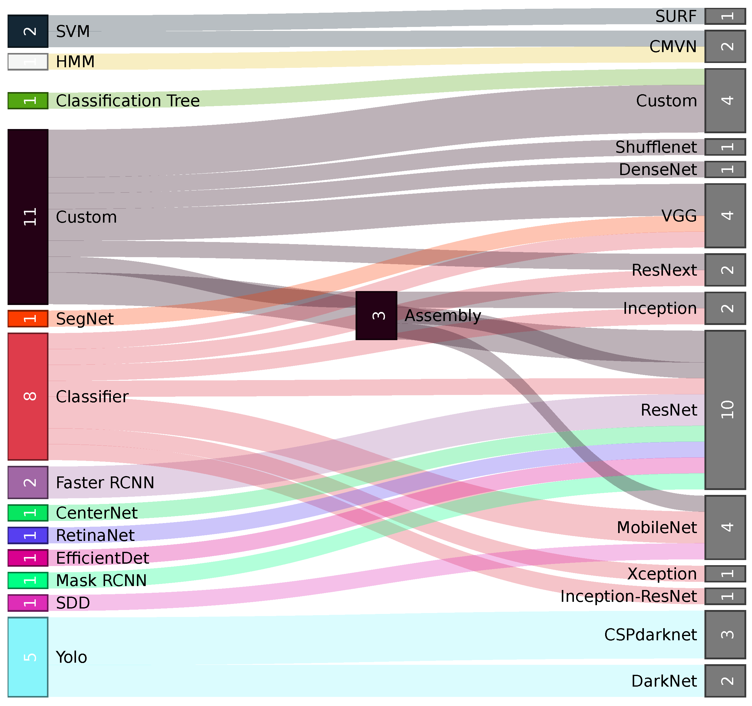
3.3. Machine Learning
- (i)
- A standard feature extractor with a tailored head. The study [7] uses a semantic retrieval model [89] placed on top of a VGG16 model to perform a four-category mapping of the 13 subcategories returned by the CNN model. Their results revealed that the proposed method achieved a significantly higher performance in waste classification (94.7% Acc.) compared to the one-stage algorithm with direct four-category predictions (69.7% Acc.). The study [52] proposes the ensemble of three classification models (InceptionV1 [90], ResNet50, MobileNetV2) trained separately. Their predictions are integrated using weights with an unequal precision measurement (UPM) strategy. The model was evaluated on Trashnet (93.5% Acc.) and Fourtrash (92.9% Acc.). Ref. [53] proposed DNN-TC, which adds two FC layers to a pretrained ResNext model. DNN-TC was evaluated on Trashnet (94% Acc.) and their dataset VN-trash (98% Acc.). Ref. [56] proposed IDRL-RWODC, a model composed of a mask region-based convolutional neural network (RCNN) [91] model with DenseNet [92] as a feature extractor that performs the waste image segmentation and passes to a deep reinforcement Q-learning algorithm for region classification. IDRL-RWODC was evaluated (99.3% Acc.) on a six-category dataset [57]. Ref. [17] developed a multi-task learning architecture (MTLA), a detection architecture with a ResNet50 backbone on which each convolutional block is applied to an attention mechanism (channel and spatial). The feature maps are passed to a feature pyramid network (FPN) with different combination strategies. The architecture was tested on the WasteRL dataset with nearly 57K images and four categories (97.2% Acc.).
- (ii)
- The improvement of an existing architecture. Ref. [39] presented GCNet, an improvement of ShuffleNetV2, by using the FReLU activation function [93], a parallel mixed attention mechanism module (PMAM), and ImageNet transfer learning. Ref. [94] presented DSCR-Net, an architecture based on Inception-V4 and ResNet that is more accurate (94.4 Acc.) than the Inception-Resnet versions [95] in a four-waste custom classification dataset.
- (iii)
- New architectures. Ref. [61] proposes using a basic CNN architecture on RGB images for plastic material classification (PS, PP, HDPE, and PET). They used the WadaBa dataset [15], a single piece of waste per image on a simple black background. Their model had a lower performance (74% Acc.) than MobileNetV2 but half the number of parameters, making it appropriate for portable devices (e.g., Raspberry Pi).
3.4. Overview of Results
4. Challenges and Limitations
- The laboratory testing: in many instances, the real-world applicability and complexity were not evaluated.
- Material identification is not enough for recycling: other inputs, such as product type and contamination, are required to define their recycling category.
- Visible-light-based approaches often result in errors due to the high similarity between materials. The majority of the proposed systems are location-specific, relying on the visual appearance of waste, which can vary significantly from one place to another.
4.1. Physical Enablers
4.2. Datasets
4.3. Machine Learning
5. Conclusions
Author Contributions
Funding
Institutional Review Board Statement
Informed Consent Statement
Data Availability Statement
Conflicts of Interest
Abbreviations
| SWM | Solid Waste Management |
| ML | Machine Learning |
| CNN | Convolutional Neural Network |
| SVM | Support Vector Machine |
| IR | Infrared |
| MSW | Municipal Solid Waste |
| SLR | Systematic Literature Review |
| CV | Computer Vision |
| ANN | Artificial Neural Network |
| HSI | Hyperspectral Imaging |
| IoT | Internet of Things |
| NIR | Near Infrared |
| RFID | Radio-Frequency Identification |
| PET | Polyethylene Terephthalate |
| PS | Polystyrene |
| PE | Polyethylene |
| PP | Polypropylene |
| RGBD | Red Green Blue Depth |
| PVC | Polyvinyl Chloride |
| HMM | Hidden Markov Model |
| FC | Fully Connected |
| MFCCs | Mel Frequency Cepstral Coefficients |
| Acc. | Average Accuracy |
| TL | Transfer Learning |
| SSD | Single Shot Detector |
| mAP | Mean Average Precision |
| IoU | Interception Over Union |
| UPM | Unequal Precision Measurement |
| RCNN | Region Convolutional Neural Network |
| FPN | Feature Pyramid Network |
| PMAM | Parallel Mixed Attention Mechanism |
| PLS-DA | Partial Least Squares Discriminant Analysis |
| Av. Rec | Average Recall |
| ASDDN | Adversarial Spatial Dropout Detection Network |
| DCGAN | Deep Convolution Generative Adversarial Network |
| GAN | Generative Adversarial Network |
Appendix A. Inclusion Criteria
- (i)
- The study’s objectives are well defined and are related to automatic waste classification.
- (ii)
- The algorithms, models, and methods used are described in detail.
- (iii)
- The classification labels belong to municipal waste recycling categories.
- (iv)
- The evaluation metrics are well described.
- (v)
- The datasets and experiments are well described (description, shape, images, or distribution of the classes).
- (vi)
- A discussion about the quality and context of the results is presented.
- (i)
- The dataset information is available (date, dimensions, etc.).
- (ii)
- The distribution of the classes is available.
- (iii)
- The labels of the dataset belong to recycling categories.
- (iv)
- The type of waste belongs to municipal, institutional, or household.
- (v)
- Examples of the observations are presented or available.
- (vi)
- A description of the dataset is available.
References
- Kaza, S.; Yao, L.; Bhada-Tata, P.; Van Woerden, F. What a Waste 2.0: A Global Snapshot of Solid Waste Management to 2050; Urban Development, World Bank Publications: Washington, DC, USA, 2018. [Google Scholar]
- Alalouch, C.; Piselli, C.; Cappa, F. Towards Implementation of Sustainability Concepts in Developing Countries; Springer: Berlin/Heidelberg, Germany, 2021. [Google Scholar]
- Wang, Z.; Lv, J.; Gu, F.; Yang, J.; Guo, J. Environmental and economic performance of an integrated municipal solid waste treatment: A Chinese case study. Sci. Total. Environ. 2020, 709, 136096. [Google Scholar] [CrossRef] [PubMed]
- Oluwadipe, S.; Garelick, H.; McCarthy, S.; Purchase, D. A critical review of household recycling barriers in the United Kingdom. Waste Manag. Res. 2021, 40, 905–918. [Google Scholar] [CrossRef] [PubMed]
- Gundupalli, S.; Hait, S.; Thakur, A. A review on automated sorting of source-separated municipal solid waste for recycling. Waste Manag. 2017, 60, 56–74. [Google Scholar] [CrossRef]
- Longo, E.; Sahin, F.A.; Redondi, A.E.; Bolzan, P.; Bianchini, M.; Maffei, S. Take the trash out… to the edge. Creating a Smart Waste Bin based on 5G Multi-access Edge Computing. In Proceedings of the GoodIT’21: Proceedings of the Conference on Information Technology for Social Good, Roma, Italy, 9–11 September 2021; pp. 55–60. [Google Scholar]
- Zhang, S.; Chen, Y.; Yang, Z.; Gong, H. Computer Vision Based Two-stage Waste Recognition-Retrieval Algorithm for Waste Classification. Resour. Conserv. Recycl. 2021, 169, 105543. [Google Scholar] [CrossRef]
- Mahat, S.; Yusoff, S.H.; Zaini, S.A.; Midi, N.S.; Mohamad, S.Y. Automatic Metal Waste Separator System In Malaysia. In Proceedings of the 2018 7th International Conference on Computer and Communication Engineering (ICCCE), Kuala Lumpur, Malaysia, 19–20 September 2018; pp. 366–371. [Google Scholar]
- Koskinopoulou, M.; Raptopoulos, F.; Papadopoulos, G.; Mavrakis, N.; Maniadakis, M. Robotic Waste Sorting Technology: Toward a Vision-Based Categorization System for the Industrial Robotic Separation of Recyclable Waste. IEEE Robot. Autom. Mag. 2021, 28, 50–60. [Google Scholar] [CrossRef]
- Wang, C.; Qin, J.; Qu, C.; Ran, X.; Liu, C.; Chen, B. A smart municipal waste management system based on deep-learning and Internet of Things. Waste Manag. 2021, 135, 20–29. [Google Scholar] [CrossRef]
- Mao, W.L.; Chen, W.C.; Fathurrahman, H.I.K.; Lin, Y.H. Deep learning networks for real-time regional domestic waste detection. J. Clean. Prod. 2022, 344, 131096. [Google Scholar] [CrossRef]
- Korucu, M.; Kaplan, O.; Buyuk, O.; Gullu, M. An investigation of the usability of sound recognition for source separation of packaging wastes in reverse vending machines. Waste Manag. 2016, 56, 46–52. [Google Scholar] [CrossRef] [PubMed]
- Calvini, R.; Orlandi, G.; Foca, G.; Ulrici, A. Developmentof a classification algorithm for efficient handling of multiple classes in sorting systems based on hyperspectral imaging. J. Spectr. Imaging 2018, 7, a13. [Google Scholar] [CrossRef]
- Kumsetty, N.V. TrashBox. 2022. Available online: https://github.com/nikhilvenkatkumsetty/TrashBox (accessed on 22 June 2022).
- Bobulski, J.; Piatkowski, J. PET waste classification method and plastic waste database - WaDaBa. Adv. Intell. Syst. Comput. 2018, 681, 57–64. [Google Scholar] [CrossRef]
- Gary Thung, M.Y. TrashNet. 2017. Available online: https://github.com/garythung/trashnet (accessed on 22 June 2022).
- Liang, S.; Gu, Y. A deep convolutional neural network to simultaneously localize and recognize waste types in images. Waste Manag. 2021, 126, 247–257. [Google Scholar] [CrossRef]
- Proença, P.F.; Simões, P. TACO: Trash annotations in context for litter detection. arXiv 2020, arXiv:2003.06975. [Google Scholar]
- Wulansari, A.; Setyanto, A.; Luthfi, E.T. Systematic Literature Review of Waste Classification Using Machine Learning. J. Inform. Telecomunication Eng. 2022, 5, 405–413. [Google Scholar] [CrossRef]
- Lu, W.; Chen, J. Computer vision for solid waste sorting: A critical review of academic research. Waste Manag. 2022, 142, 29–43. [Google Scholar] [CrossRef]
- Guo, H.N.; Wu, S.B.; Tian, Y.J.; Zhang, J.; Liu, H.T. Application of machine learning methods for the prediction of organic solid waste treatment and recycling processes: A review. Bioresour. Technol. 2021, 319, 124114. [Google Scholar] [CrossRef]
- Erkinay Ozdemir, M.; Ali, Z.; Subeshan, B.; Asmatulu, E. Applying machine learning approach in recycling. J. Mater. Cycles Waste Manag. 2021, 23, 855–871. [Google Scholar] [CrossRef]
- Flores, M.G.; Tan, J.B., Jr. Literature review of automated waste segregation system using machine learning: A comprehensive analysis. Int. J. Simulation: Syst. Sci. Technol. 2019, 11, 15.1–15.7. [Google Scholar] [CrossRef]
- Alcaraz-Londoño, L.M.; Ortiz-Clavijo, L.F.; Duque, C.J.G.; Betancur, S.A.G. Review on techniques of automatic solid waste separation in domestics applications. Bull. Electr. Eng. Inform. 2022, 11, 128–133. [Google Scholar] [CrossRef]
- Zhang, X.; Liu, C.; Chen, Y.; Zheng, G.; Chen, Y. Source separation, transportation, pretreatment, and valorization of municipal solid waste: A critical review. Environ. Dev. Sustain. 2021, 24, 11471–11513. [Google Scholar] [CrossRef]
- Keerthana, S.; Kiruthika, B.; Lokeshvaran, R.; Midhunchakkaravarthi, B.; Dhivyasri, G. A Review on Smart Waste Collection and Disposal System. J. Phys. Conf. Ser. 2021, 1969, 012029. [Google Scholar] [CrossRef]
- Abdallah, M.; Talib, M.A.; Feroz, S.; Nasir, Q.; Abdalla, H.; Mahfood, B. Artificial intelligence applications in solid waste management: A systematic research review. Waste Manag. 2020, 109, 231–246. [Google Scholar] [CrossRef]
- Carpenteros, A.; Capinig, E.; Bagaforo, J.; Edris, Y.; Samonte, M. An Evaluation of Automated Waste Segregation Systems: A Usability Literature Review. In Proceedings of the ICIEB’21: Proceedings of the 2021 2nd International Conference on Internet and E-Business, Barcelona, Spain, 9–11 June 2021; pp. 22–28. [Google Scholar] [CrossRef]
- Barbara Kitchenham; Stuart Charters. Guidelines for Performing Systematic Literature Reviews in Software Engineering; Keele University: Keele, UK, 2007. [Google Scholar]
- Tamin, O.; Moung, E.G.; Dargham, J.A.; Yahya, F.; Omatu, S. A review of hyperspectral imaging-based plastic waste detection state-of-the-arts. Int. J. Electr. Comput. Eng. (IJECE) 2023, 13, 3407–3419. [Google Scholar] [CrossRef]
- Lubongo, C.; Alexandridis, P. Assessment of performance and challenges in use of commercial automated sorting technology for plastic waste. Recycling 2022, 7, 11. [Google Scholar] [CrossRef]
- Mohamed, N.H.; Khan, S.; Jagtap, S. Modernizing Medical Waste Management: Unleashing the Power of the Internet of Things (IoT). Sustainability 2023, 15, 9909. [Google Scholar] [CrossRef]
- Jagtap, S.; Bhatt, C.; Thik, J.; Rahimifard, S. Monitoring potato waste in food manufacturing using image processing and internet of things approach. Sustainability 2019, 11, 3173. [Google Scholar] [CrossRef]
- Paulraj, S.; Hait, S.; Thakur, A. Automated municipal solid waste sorting for recycling using a mobile manipulator. In Proceedings of the ASME 2016 International Design Engineering Technical Conference (IDETC), Charlotte, NC, USA, 21–24 August 2016; p. 5A-2016. [Google Scholar] [CrossRef]
- Kim, D.; Lee, S.; Park, M.; Lee, K.; Kim, D.Y. Designing of reverse vending machine to improve its sorting efficiency for recyclable materials for its application in convenience stores. J. Air Waste Manag. Assoc. 2021, 71, 1312–1318. [Google Scholar] [CrossRef] [PubMed]
- Kapadia, H.; Patel, A.; Patel, J.; Patidar, S.; Richhriya, Y.; Trivedi, D.; Patel, P.; Mehta, M. Dry waste segregation using seamless integration of deep learning and industrial machine vision. In Proceedings of the 2021 IEEE International Conference on Electronics, Computing and Communication Technologies (CONECCT), Bangalore, India, 9–11 July 2021; pp. 1–7. [Google Scholar]
- Ziouzios, D.; Baras, N.; Balafas, V.; Dasygenis, M.; Stimoniaris, A. Intelligent and Real-Time Detection and Classification Algorithm for Recycled Materials Using Convolutional Neural Networks. Recycling 2022, 7, 9. [Google Scholar] [CrossRef]
- Rahman, M.; Islam, R.; Hasan, A.; Bithi, N.; Hasan, M.; Rahman, M. Intelligent waste management system using deep learning with IoT. J. King Saud Univ.—Comput. Inf. Sci. 2020, 34, 2072–2087. [Google Scholar] [CrossRef]
- Chen, Z.; Yang, J.; Chen, L.; Jiao, H. Garbage classification system based on improved ShuffleNet v2. Resour. Conserv. Recycl. 2022, 178, 106090. [Google Scholar] [CrossRef]
- Midi, N.; Rahmad, M.; Yusoff, S.; Mohamad, S. Recyclable waste separation system based on material classification using weight and size of waste. Bull. Electr. Eng. Inform. 2019, 8, 477–487. [Google Scholar] [CrossRef]
- Md, R.; Sayed, R.H.; Kowshik, A.K. Intelligent Waste Sorting Bin for Recyclable Municipal Solid Waste. In Proceedings of the 2021 International Conference on Automation, Control and Mechatronics for Industry 4.0 (ACMI), Rajshahi, Bangladesh, 8–9 July 2021; pp. 1–5. [Google Scholar]
- Chandramohan, A.; Mendonca, J.; Shankar, N.; Baheti, N.; Krishnan, N.; Suma, M. Automated Waste Segregator. In Proceedings of the 2014 Texas Instruments India Educators Conference, TIIEC 2014, Bangalore, Karnataka, 4–5 April 2014; pp. 1–6. [Google Scholar] [CrossRef]
- Maulana, F.; Widyanto, T.; Pratama, Y.; Mutijarsa, K. Design and Development of Smart Trash Bin Prototype for Municipal Solid Waste Management. In Proceedings of the 2018 International Conference on ICT for Smart Society (ICISS), Semarang, Indonesia, 10–11 October 2018. [Google Scholar] [CrossRef]
- Funch, O.; Marhaug, R.; Kohtala, S.; Steinert, M. Detecting glass and metal in consumer trash bags during waste collection using convolutional neural networks. Waste Manag. 2021, 119, 30–38. [Google Scholar] [CrossRef]
- Lu, G.; Wang, Y.; Xu, H.; Yang, H.; Zou, J. Deep multimodal learning for municipal solid waste sorting. Sci. China Technol. Sci. 2022, 65, 324–335. [Google Scholar] [CrossRef]
- Seredkin, A.; Tokarev, M.; Plohih, I.; Gobyzov, O.; Markovich, D. Development of a method of detection and classification of waste objects on a conveyor for a robotic sorting system. J. Phys. Conf. Ser. 2019, 1359, 012127. [Google Scholar] [CrossRef]
- Melinte, D.; Travediu, A.M.; Dumitriu, D. Deep convolutional neural networks object detector for real-time waste identification. Appl. Sci. 2020, 10, 7301. [Google Scholar] [CrossRef]
- Andhy Panca Saputra, K. Waste Object Detection and Classification using Deep Learning Algorithm: YOLOv4 and YOLOv4-tiny. Turk. J. Comput. Math. Educ. (TURCOMAT) 2021, 12, 5583–5595. [Google Scholar]
- Aqyuni, U.; Endah, S.; Sasongko, P.; Kusumaningrum, R.; Khadijah; Rismiyati; Rasyidi, H. Waste Image Segmentation Using Convolutional Neural Network Encoder-Decoder with SegNet Architecture. In Proceedings of the 2020 4th International Conference on Informatics and Computational Sciences (ICICoS), Semarang, Indonesia, 10–11 November 2020. [CrossRef]
- Lin, T.Y.; Maire, M.; Belongie, S.; Hays, J.; Perona, P.; Ramanan, D.; Dollár, P.; Zitnick, C.L. Microsoft coco: Common objects in context. In Proceedings of the Computer Vision—ECCV 2014, 13th European Conference, Zurich, Switzerland, 6–12 September 2014; pp. 740–755. [Google Scholar]
- Singh, S.; Gautam, J.; Rawat, S.; Gupta, V.; Kumar, G.; Verma, L. Evaluation of Transfer Learning based Deep Learning architectures for Waste Classification. In Proceedings of the 2021 4th International Symposium on Advanced Electrical and Communication Technologies (ISAECT), Alkhobar, Saudi Arabia, 6–8 December 2021. [Google Scholar] [CrossRef]
- Zheng, H.; Gu, Y. Encnn-upmws: Waste classification by a CNN ensemble using the UPM weighting strategy. Electronics 2021, 10, 427. [Google Scholar] [CrossRef]
- Vo, A.H.; Vo, M.T.; Le, T. A novel framework for trash classification using deep transfer learning. IEEE Access 2019, 7, 178631–178639. [Google Scholar] [CrossRef]
- Qin, L.W.; Ahmad, M.; Ali, I.; Mumtaz, R.; Zaidi, S.M.H.; Alshamrani, S.S.; Raza, M.A.; Tahir, M. Precision measurement for industry 4.0 standards towards solid waste classification through enhanced imaging sensors and deep learning model. Wirel. Commun. Mob. Comput. 2021, 2021, 9963999. [Google Scholar] [CrossRef]
- Caballero, J.; Vergara, F.; Miranda, R.; Serracín, J. Inference of Recyclable Objects with Convolutional Neural Networks. arXiv 2021, arXiv:2104.00868. [Google Scholar]
- Duhayyim, M.; Eisa, T.; Al-Wesabi, F.; Abdelmaboud, A.; Hamza, M.; Zamani, A.; Rizwanullah, M.; Marzouk, R. Deep Reinforcement Learning Enabled Smart City Recycling Waste Object Classification. Comput. Mater. Contin. 2022, 71, 5699–5715. [Google Scholar] [CrossRef]
- Cchangcs. Garbage Classification. 2019. Available online: https://www.kaggle.com/datasets/asdasdasasdas/garbage-classification (accessed on 22 June 2022).
- Frost, S.; Tor, B.; Agrawal, R.; Forbes, A.G. Compostnet: An image classifier for meal waste. In Proceedings of the 2019 IEEE Global Humanitarian Technology Conference (GHTC), Seattle, WA, USA, 17–20 October 2019; pp. 1–4. [Google Scholar]
- Thanawala, D.; Sarin, A.; Verma, P. An Approach to Waste Segregation and Management Using Convolutional Neural Networks. Commun. Comput. Inf. Sci. 2020, 1244, 139–150. [Google Scholar] [CrossRef]
- Pal, S. Waste Classification Data v2. 2020. Available online: https://www.kaggle.com/datasets/sapal6/waste-classification-data-v2 (accessed on 22 June 2022).
- Bobulski, J.; Kubanek, M. Deep Learning for Plastic Waste Classification System. Appl. Comput. Intell. Soft Comput. 2021, 2021, 6626948. [Google Scholar] [CrossRef]
- Sekar, S. Waste Classification Data. 2019. Available online: https://www.kaggle.com/datasets/techsash/waste-classification-data (accessed on 22 June 2022).
- Mohamed, M. Garbage Classification (12 Classes). 2021. Available online: https://www.kaggle.com/datasets/mostafaabla/garbage-classification (accessed on 22 June 2022).
- Koca, H.S. Recyclable Solid Waste Dataset. 2021. Available online: https://www.kaggle.com/datasets/hseyinsaidkoca/recyclable-solid-waste-dataset-on-5-background-co (accessed on 22 June 2022).
- Lv, Z.; Li, H.; Liu, Y. Garbage detection and classification method based on YoloV5 algorithm. In Proceedings of the Fourteenth International Conference on Machine Vision (ICMV 2021), Rome, Italy, 8–12 November 2021; SPIE: Bellingham, WA, USA, 2022; Volume 12084, p. 4. [Google Scholar]
- Panwar, H.; Gupta, P.; Siddiqui, M.K.; Morales-Menendez, R.; Bhardwaj, P.; Sharma, S.; Sarker, I.H. AquaVision: Automating the detection of waste in water bodies using deep transfer learning. Case Stud. Chem. Environ. Eng. 2020, 2, 100026. [Google Scholar] [CrossRef]
- Hong, J.; Fulton, M.; Sattar, J. Trashcan: A semantically-segmented dataset towards visual detection of marine debris. arXiv 2020, arXiv:2007.08097. [Google Scholar]
- Wang, T.; Cai, Y.; Liang, L.; Ye, D. A multi-level approach to waste object segmentation. Sensors 2020, 20, 3816. [Google Scholar] [CrossRef] [PubMed]
- Kraft, M.; Piechocki, M.; Ptak, B.; Walas, K. Autonomous, onboard vision-based trash and litter detection in low altitude aerial images collected by an unmanned aerial vehicle. Remote. Sens. 2021, 13, 965. [Google Scholar] [CrossRef]
- Serezhkin, A. Drinking Waste Classification. 2021. Available online: https://www.kaggle.com/datasets/arkadiyhacks/drinking-waste-classification (accessed on 22 June 2022).
- Khalid, S.; Khalil, T.; Nasreen, S. A survey of feature selection and feature extraction techniques in machine learning. In Proceedings of the 2014 Science and Information Conference, London, UK, 27–29 August 2014; pp. 372–378. [Google Scholar]
- Käding, C.; Rodner, E.; Freytag, A.; Denzler, J. Fine-tuning deep neural networks in continuous learning scenarios. In Proceedings of the Computer Vision—ACCV 2016 Workshops: ACCV 2016 International Workshops, Taipei, Taiwan, 20–24 November 2016; pp. 588–605. [Google Scholar]
- Simonyan, K.; Zisserman, A. Very deep convolutional networks for large-scale image recognition. arXiv 2014, arXiv:1409.1556. [Google Scholar]
- Xie, S.; Girshick, R.; Dollár, P.; Tu, Z.; He, K. Aggregated residual transformations for deep neural networks. In Proceedings of the 2017 IEEE conference on Computer Vision and Pattern Recognition, Honolulu, HI, USA, 21–26 July 2017; pp. 1492–1500. [Google Scholar]
- Russakovsky, O.; Deng, J.; Su, H.; Krause, J.; Satheesh, S.; Ma, S.; Huang, Z.; Karpathy, A.; Khosla, A.; Bernstein, M.; et al. Imagenet large scale visual recognition challenge. Int. J. Comput. Vis. 2015, 115, 211–252. [Google Scholar] [CrossRef]
- Liu, W.; Anguelov, D.; Erhan, D.; Szegedy, C.; Reed, S.; Fu, C.Y.; Berg, A.C. Ssd: Single shot multibox detector. In Proceedings of the Computer Vision—ECCV 2016: 14th European Conference, Amsterdam, The Netherlands, 11–14 October 2016; pp. 21–37. [Google Scholar]
- Sandler, M.; Howard, A.; Zhu, M.; Zhmoginov, A.; Chen, L.C. Mobilenetv2: Inverted residuals and linear bottlenecks. In Proceedings of the 2018 IEEE Conference on Computer Vision and Pattern Recognition, Salt Lake City, UT, USA, 18–23 June 2018; pp. 4510–4520. [Google Scholar]
- Redmon, J.; Farhadi, A. Yolov3: An incremental improvement. arXiv 2018, arXiv:1804.02767. [Google Scholar]
- Bochkovskiy, A.; Wang, C.Y.; Liao, H.Y.M. Yolov4: Optimal speed and accuracy of object detection. arXiv 2020, arXiv:2004.10934. [Google Scholar]
- Badrinarayanan, V.; Kendall, A.; Cipolla, R. Segnet: A deep convolutional encoder-decoder architecture for image segmentation. IEEE Trans. Pattern Anal. Mach. Intell. 2017, 39, 2481–2495. [Google Scholar] [CrossRef] [PubMed]
- Jocher, G. YoloV5. 2020. Available online: https://github.com/ultralytics/yolov5 (accessed on 22 June 2022).
- Lin, T.Y.; Goyal, P.; Girshick, R.; He, K.; Dollár, P. Focal loss for dense object detection. In Proceedings of the IEEE International Conference on Computer Vision, Venice, Italy, 22–29 October 2017; pp. 2980–2988. [Google Scholar]
- Targ, S.; Almeida, D.; Lyman, K. Resnet in resnet: Generalizing residual architectures. arXiv 2016, arXiv:1603.08029. [Google Scholar]
- Chen, Y.; Sun, J.; Bi, S.; Meng, C.; Guo, F. Multi-objective solid waste classification and identification model based on transfer learning method. J. Mater. Cycles Waste Manag. 2021, 23, 2179–2191. [Google Scholar] [CrossRef]
- Majchrowska, S.; Miko\lajczyk, A.; Ferlin, M.; Klawikowska, Z.; Plantykow, M.A.; Kwasigroch, A.; Majek, K. Waste detection in Pomerania: Non-profit project for detecting waste in environment. arXiv 2021, arXiv:2105.06808. [Google Scholar]
- Feng, B.; Ren, K.; Tao, Q.; Gao, X. A robust waste detection method based on cascade adversarial spatial dropout detection network. In Proceedings of the Optoelectronic Imaging and Multimedia Technology VII, Online Only, China, 11–16 October 2020; SPIE: Bellingham, WA, USA, 2020; Volume 11550. [Google Scholar] [CrossRef]
- Mingyang, L.; Chengrong, L. Research on Household Waste Detection System Based on Deep Learning. In Proceedings of the 7th International Conference on Energy Science and Chemical Engineering (ICESCE 2021), Dali, China, 21–23 May 2021; Volume 267. [Google Scholar]
- Cai, H.; Cao, X.; Huang, L.; Zou, L.; Yang, S. Research on Computer Vision-Based Waste Sorting System. In Proceedings of the 2020 5th International Conference on Control, Robotics and Cybernetics (CRC), Wuhan, China, 16–18 October 2020; pp. 117–122. [Google Scholar] [CrossRef]
- Mikolov, T.; Chen, K.; Corrado, G.; Dean, J. Efficient estimation of word representations in vector space. arXiv 2013, arXiv:1301.3781. [Google Scholar]
- Szegedy, C.; Liu, W.; Jia, Y.; Sermanet, P.; Reed, S.; Anguelov, D.; Erhan, D.; Vanhoucke, V.; Rabinovich, A. Going deeper with convolutions. In Proceedings of the 2015 IEEE Conference on Computer Vision and Pattern Recognition, Boston, MA, USA, 7–12 June 2015; pp. 1–9. [Google Scholar]
- Girshick, R.; Donahue, J.; Darrell, T.; Malik, J. Rich feature hierarchies for accurate object detection and semantic segmentation. In Proceedings of the 2014 IEEE Conference on Computer Vision and Pattern Recognition, Columbus, OH, USA, 23–28 June 2014; pp. 580–587. [Google Scholar]
- Huang, G.; Liu, Z.; Van Der Maaten, L.; Weinberger, K.Q. Densely connected convolutional networks. In Proceedings of the 2017 IEEE Conference on Computer Vision and Pattern Recognition, Honolulu, HI, USA, 21–26 July 2017; pp. 4700–4708. [Google Scholar]
- Ma, N.; Zhang, X.; Sun, J. Funnel activation for visual recognition. In Proceedings of the Computer Vision—ECCV 2020: 16th European Conference, Glasgow, UK, 23–28 August 2020; pp. 351–368. [Google Scholar]
- Song, F.; Zhang, Y.; Zhang, J. Optimization of CNN-based Garbage Classification Model. In Proceedings of the 4th International Conference on Computer Science and Application Engineering, Sanya, China, 20–22 October 2020. [Google Scholar] [CrossRef]
- Szegedy, C.; Ioffe, S.; Vanhoucke, V.; Alemi, A.A. Inception-v4, inception-resnet and the impact of residual connections on learning. In Proceedings of the AAAI Conference on Artificial Intelligence, San Francisco, CA, USA, 4–9 February 2017. [Google Scholar]
- Zhang, Q.; Yang, Q.; Zhang, X.; Wei, W.; Bao, Q.; Su, J.; Liu, X. A multi-label waste detection model based on transfer learning. Resour. Conserv. Recycl. 2022, 181, 106235. [Google Scholar] [CrossRef]
- Krichen, M. Convolutional Neural Networks: A Survey. Computers 2023, 12, 151. [Google Scholar] [CrossRef]
- Bay, H.; Tuytelaars, T.; Gool, L.V. Surf: Speeded up robust features. In Proceedings of the Computer Vision—ECCV 2006: 9th European Conference on Computer Vision, Graz, Austria, 7–13 May 2006; pp. 404–417. [Google Scholar]
- Young, S.; Evermann, G.; Gales, M.; Hain, T.; Kershaw, D.; Liu, X.; Moore, G.; Odell, J.; Ollason, D.; Povey, D.; et al. The HTK Book; Cambridge University Engineering Department: Cambridge, UK, 2002; Volume 3, p. 12. [Google Scholar]
- Fan, J.; Cui, L.; Fei, S. Waste Detection System Based on Data Augmentation and YOLO_EC. Sensors 2023, 23, 3646. [Google Scholar] [CrossRef]
- Kumsetty, N.V.; Nekkare, A.B.; Sowmya Kamath, S.; Anand Kumar, M. An Approach for Waste Classification Using Data Augmentation and Transfer Learning Models. In Machine Vision and Augmented Intelligence: Select Proceedings of MAI 2022; Springer Nature: Singapore, 2023; pp. 357–368. [Google Scholar]
- Wu, H.; Zheng, S.; Zhang, J.; Huang, K. Gp-gan: Towards realistic high-resolution image blending. In Proceedings of the MM’19: The 27th ACM International Conference on Multimedia, Nice, France, 21–25 October 2019; pp. 2487–2495. [Google Scholar]
- Zhang, Q.; Yang, Q.; Zhang, X.; Bao, Q.; Su, J.; Liu, X. Waste image classification based on transfer learning and convolutional neural network. Waste Manag. 2021, 135, 150–157. [Google Scholar] [CrossRef] [PubMed]


| Ref. | Year | Subject |
|---|---|---|
| [30] | 2023 | A review of state-of-the-art hyperspectral imaging-based plastic waste detection |
| [19] | 2022 | Computer vision (CV) for waste classification |
| [24] | 2022 | Trends in household waste recycling |
| [20] | 2022 | Critical review of CV-enabled MSW sorting |
| [25] | 2021 | Critical review of MSW management strategies |
| [21] | 2021 | Review on ML for solid organic waste treatment |
| [22] | 2021 | ML algorithms used in recycling systems |
| [28] | 2021 | Effectiveness, advantages, and disadvantages, of automated waste segregation systems |
| [26] | 2021 | Monitoring methods, garbage disposal techniques, and technologies |
| [27] | 2020 | SLR on forecasting of waste characteristics, waste bin level detection, process parameters prediction, vehicle routing, and SWM planning |
| [23] | 2019 | Strengths and weaknesses of waste segregation algorithms |
| [5] | 2017 | Physical processes, sensors, actuators, control, and autonomy |
| Criteria | ID | Terms | |||
|---|---|---|---|---|---|
| Population | A | Waste | Disposal | ||
| Intervention | B | Model | Automat * | ||
| C | System | ||||
| Comparison | D | None | |||
| Outcome | E | Detection | Classification | Separation | Sorting |
| Context | F | Municipal | Household | Domestic | |
| ID | Question | Query |
|---|---|---|
| Q1 | Which are the devices (physical enablers) used for municipal indirect waste separation systems? | A and (C W/5 E) and F |
| Q2 | What are the datasets used for developing waste separation systems? | A and DATASET * and E and F |
| Q3 | What machine learning techniques are used in automatic waste separation systems? | A and (B W/5 E) and F |
Disclaimer/Publisher’s Note: The statements, opinions and data contained in all publications are solely those of the individual author(s) and contributor(s) and not of MDPI and/or the editor(s). MDPI and/or the editor(s) disclaim responsibility for any injury to people or property resulting from any ideas, methods, instructions or products referred to in the content. |
© 2023 by the authors. Licensee MDPI, Basel, Switzerland. This article is an open access article distributed under the terms and conditions of the Creative Commons Attribution (CC BY) license (https://creativecommons.org/licenses/by/4.0/).
Share and Cite
Arbeláez-Estrada, J.C.; Vallejo, P.; Aguilar, J.; Tabares-Betancur, M.S.; Ríos-Zapata, D.; Ruiz-Arenas, S.; Rendón-Vélez, E. A Systematic Literature Review of Waste Identification in Automatic Separation Systems. Recycling 2023, 8, 86. https://doi.org/10.3390/recycling8060086
Arbeláez-Estrada JC, Vallejo P, Aguilar J, Tabares-Betancur MS, Ríos-Zapata D, Ruiz-Arenas S, Rendón-Vélez E. A Systematic Literature Review of Waste Identification in Automatic Separation Systems. Recycling. 2023; 8(6):86. https://doi.org/10.3390/recycling8060086
Chicago/Turabian StyleArbeláez-Estrada, Juan Carlos, Paola Vallejo, Jose Aguilar, Marta Silvia Tabares-Betancur, David Ríos-Zapata, Santiago Ruiz-Arenas, and Elizabeth Rendón-Vélez. 2023. "A Systematic Literature Review of Waste Identification in Automatic Separation Systems" Recycling 8, no. 6: 86. https://doi.org/10.3390/recycling8060086
APA StyleArbeláez-Estrada, J. C., Vallejo, P., Aguilar, J., Tabares-Betancur, M. S., Ríos-Zapata, D., Ruiz-Arenas, S., & Rendón-Vélez, E. (2023). A Systematic Literature Review of Waste Identification in Automatic Separation Systems. Recycling, 8(6), 86. https://doi.org/10.3390/recycling8060086