An Experimental Approach to Determining the Average Diffusion Coefficient of Volatile Components in Polymer Waste Materials

Abstract

One of the major challenges in recycling plastics is the removal of undesired volatile components from the polymeric phase, which may reduce process efficiency and negatively affect product quality. Accordingly, the recycling industry employs a broad range of degassing techniques, the efficiency of which often depends on the diffusion coefficient—a measure of the mass transport of volatile components in polymeric phases. The aim of this study was to develop a practically feasible experimental approach using thermogravimetric analysis (TGA) to determine the average diffusion coefficient of volatile components in polymer waste materials. First, the TGA method was validated with a pressure decay apparatus (PDA) using predefined binary material mixtures: Thin sheets were pressed from virgin high-density polyethylene (HDPE) and polypropylene (PP) and deliberately saturated with toluene in a sorption experiment. These saturated samples were then used in TGA and PDA desorption experiments at 60 °C, 80 °C and 100 °C, which yielded similar results with an average difference of 7.4% for the HDPE-toluene system and 14.7% for the PP-toluene system. When validated, TGA was employed to determine the diffusion coefficient of volatile components in post-industrial plastic waste melt at a temperature of 220 °C. The proposed method contributes to the understanding of diffusion-based mass transport in polymer waste materials and provides a key parameter for model-based process control and optimization. In practice, the diffusion coefficient results can be used to predict the degassing performance of an extrusion process in the mechanical recycling of plastic waste.

1. Introduction

The demand for plastics remains undiminished. After a brief period of stagnation in 2020, global plastics production increased again and reached a new peak of 390.7 Mt in 2022. The largest consumer of plastics in Europe by far is the packaging sector with 39.1%, followed by the building and construction sector with 21.3% and the automotive industry with 8.6% [1]. In a 2008 directive, the European Parliament issued guidelines for member states to increase the rates of reuse and recycling of waste materials, with the target of reaching a 55% recycling rate by 2025 and a 60% rate by 2030 [2]. Further, with a 2018 decision, the European Parliament urged the European Commission to revise and strengthen the general requirements of the Packaging and Packaging Waste Directives (PPWD) by the end of 2020 to implement the circular economy strategy in the plastics industry. Although legislative pressure on the plastics industry has recently increased, the proportion of recycled plastics in the EU stagnates at roughly 8% [1]. If the above targets are to be achieved, the recycling of plastics will become increasingly important, and plastic as a material must be shifted into a sustainable circular economy [3]. Life-cycle analyses (LCAs) have shown that beverages multi-packaged in post-consumer recycled plastic cause 73% less greenhouse gas emissions and consume 90% less energy than their cardboard counterparts [4]. These results accord with the goals of the European Green Deal, which aims to reduce greenhouse gases to 45% of the 1990 levels by 2030 and to achieve climate neutrality by 2050 [5,6].

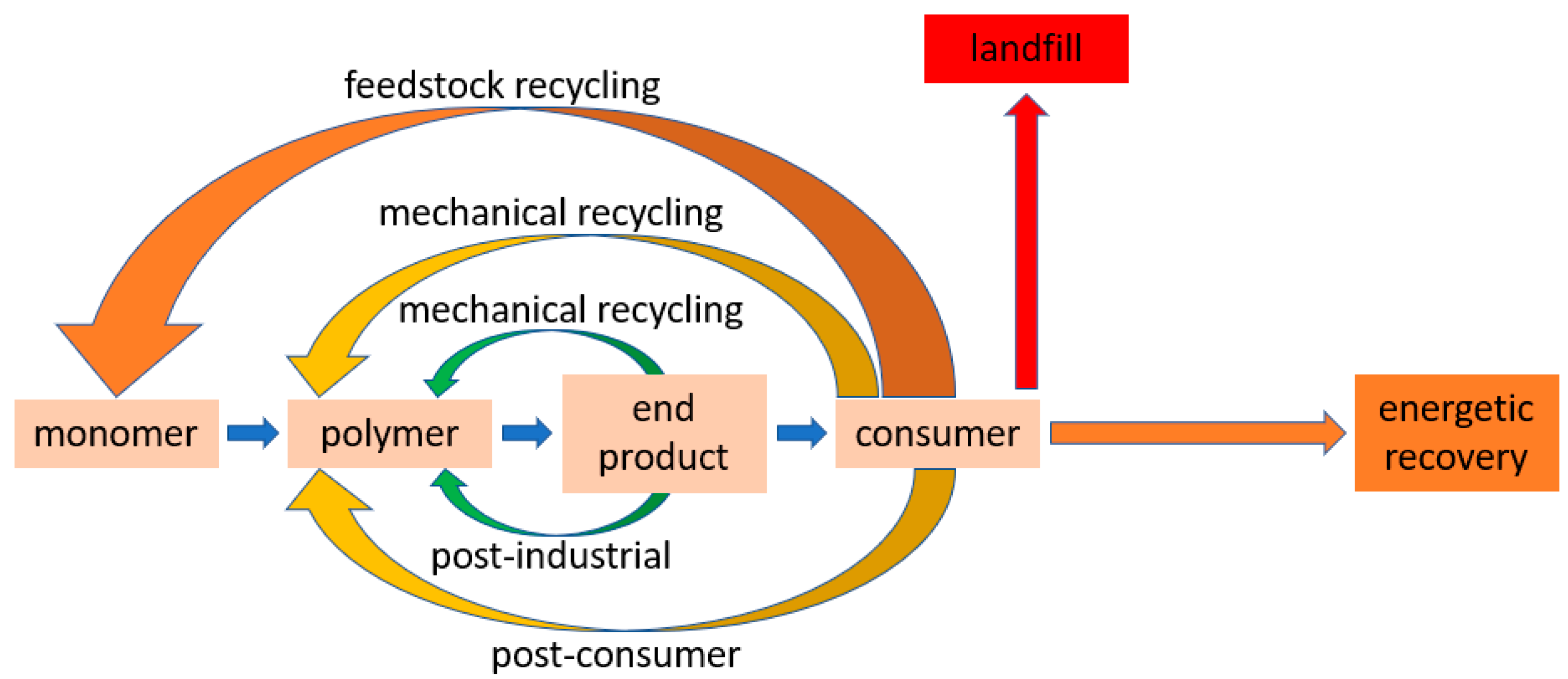
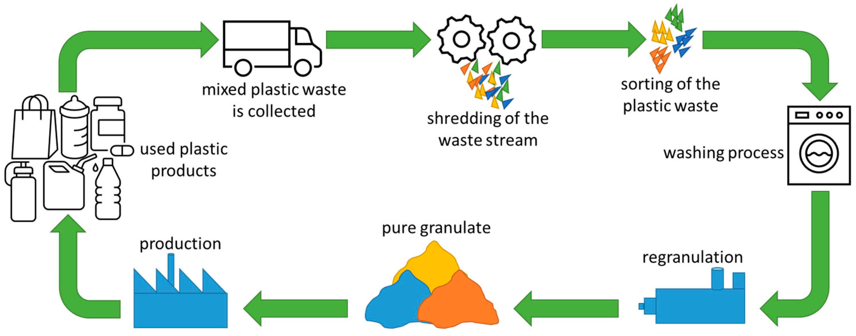
Fundamentally, distinctions are made between post-industrial and post-consumer plastic waste and between the recovery and recycling terms (Figure 1). Post-consumer waste is generated by the end consumer, while post-industrial waste is generated during production. Recovery is a generic term and describes all ways of recovering plastic waste. Recycling is a sub-term and describes all options of material reuse and resource recycling.

Figure 2 shows an overview of a mechanical recycling process. Post-consumer plastic waste is commonly collected by disposal companies. The plastic waste is often shredded before it is sent to a sorting process, where it is initially roughly sorted according to density, shape, size, and color [7,8,9]. Here, ferrous metals, for example, can be separated from the waste stream by using a magnet. Paper and label scraps are typically separated from plastics in an air classifier. A vibrating sieve can be employed to sort by size, and optical sensors detect color differences. The waste is then sorted automatically by polymer type, most commonly by means of near-infrared (NIR) spectroscopy. This optical surface technique, however, has problems with detecting black or very dark surfaces and potentially with multilayer films [10,11]. The sorted plastic waste is then sent for washing, where organic and adhesive residues and cellulose fibers are removed using media such as hot or cold water, with or without the addition of chemicals.

In the next step, the pretreated plastic waste is converted into granules in an extrusion or compounding process, where material quality can be improved, for example, by filtration or degassing and by the targeted addition of virgin materials or additives. In mechanical recycling, extrusion is the most important process for the regranulation of plastic waste. The direct processing of preconditioned plastic waste is often problematic due to the low bulk density of regrind and film material and the material variability of the input stream, especially in post-consumer waste. The end product made from recyclate is returned to the consumer, thus closing the material cycle. Consistently high recyclate quality is a basic requirement for achieving high recycling rates in future.

Products made of plastic come in different colors, and much plastic waste is also contaminated with volatile substances. This may not only affect the quality of the finished product; the product may also smell unpleasant and thus fail to meet the consumer’s expectations. In addition, plastic products entering the recycling chain have usually been exposed to combinations of various environmental influences during their service life, such as heat, light, moisture and oxygen, and mechanical stress, which causes material degradation by photooxidation processes [12]. Material degradation, due to thermomechanical processes both in use and in processing, results in the formation of low-molecular-weight volatile compounds, which are commonly referred to as volatile organic compounds (VOCs). These VOCs can affect not only the product properties (e.g., bubble formation and poorer mechanical performance), but also manufacturing processes (e.g., strong foaming of the melt and corrosion of the processing machine). A critical step in many polymer processing operations is therefore degassing—the removal of volatile components, such as reaction by-products, residual monomers, solvents, moisture and other impurities, from the polymeric phase [13]. For this purpose, various methods and devices are available in industries, which can be classified into two main categories: (i) rotating devolatilizers (e.g., vented extruders) and (ii) non-rotating devolatilizers (e.g., falling-strand devolatilizers) [14]. Although polymers can be degassed in the solid state (e.g., the removal of odors during the drying process), volatile components are often removed from the melt phase because VOCs evaporate more easily in this aggregate state (e.g., devolatilization in a degassing extruder). In this context, extrusion (and compounding) is of particular importance, where vacuum is used to extract volatile components via free surfaces in a partially filled screw channel.

There are two mechanisms that describe the mass transfer of volatile substances in polymeric phases: (i) diffusion-dominated film degassing and (ii) bubble-dominated foam degassing [15]. For bubble forming, the material must be supersaturated with volatile components and subjected to shear stress. In general, foam degassing is more efficient than film degassing because the free surfaces for volatilization of unwanted substances are many times larger [16]. In regranulation processes, mass transfer is commonly assumed to be diffusion-driven [14,15,17,18]. The diffusion coefficient describes the mass transport of molecules due to their random motion [19,20] and is a measure of the velocity at which diffusion processes occur. Regardless of whether the mass transport is diffusion-based (film degassing) or bubble-dominated (foam degassing), a proportion of mass is always transported via diffusion. From a general viewpoint, there is no universal measurement technique for determining, experimentally, the diffusion coefficients of VOCs in polymeric matrices. The diffusion coefficient depends on various variables, including (i) the molecular size of the diffusing substance, (ii) temperature, (iii) pressure, (iv) the viscosities of the medium in which the substance diffuses and (v) the concentration of the diffusing substance. The effects of these parameters depend on the aggregate state of the medium in which the molecules move, that is, in gas, liquid or solid [21]. The measurement of mass transfer properties is complex because it is difficult to measure the concentrations of volatile substances. Existing experimental techniques can be divided into direct and indirect methods [22]:

• Direct methods determine the diffusion coefficient by measuring the concentration of the diffusing substance as a function of penetration depth. These methods are based directly on Fick’s diffusion laws.
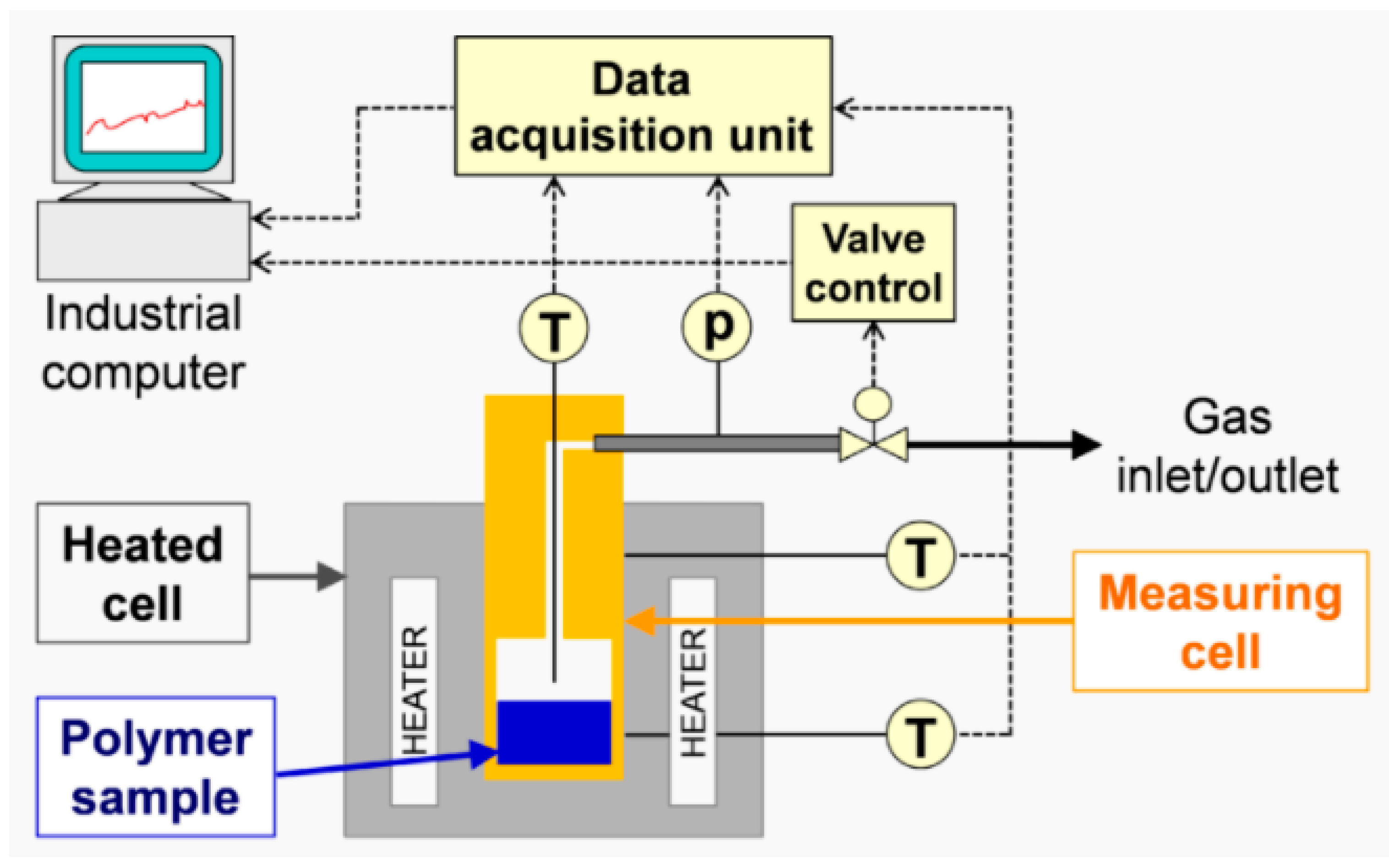
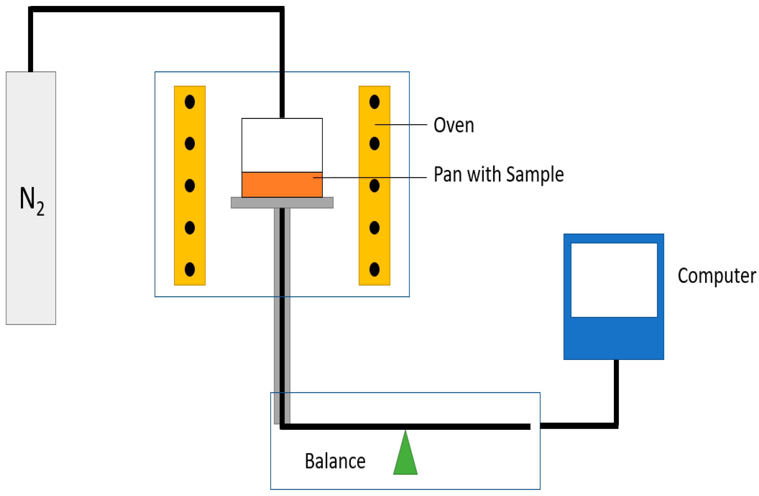
• Indirect methods measure the changes in a parameter that depends on the rate of diffusion, for instance, the rate of change in solution volume or the movement of the interface (e.g., gas–liquid interface), the rate of pressure drop in a closed cell or the rate of mass loss in a closed cell. The two techniques used in this study, thermogravimetric analysis (TGA) and pressure decay apparatus (PDA), are also indirect methods.

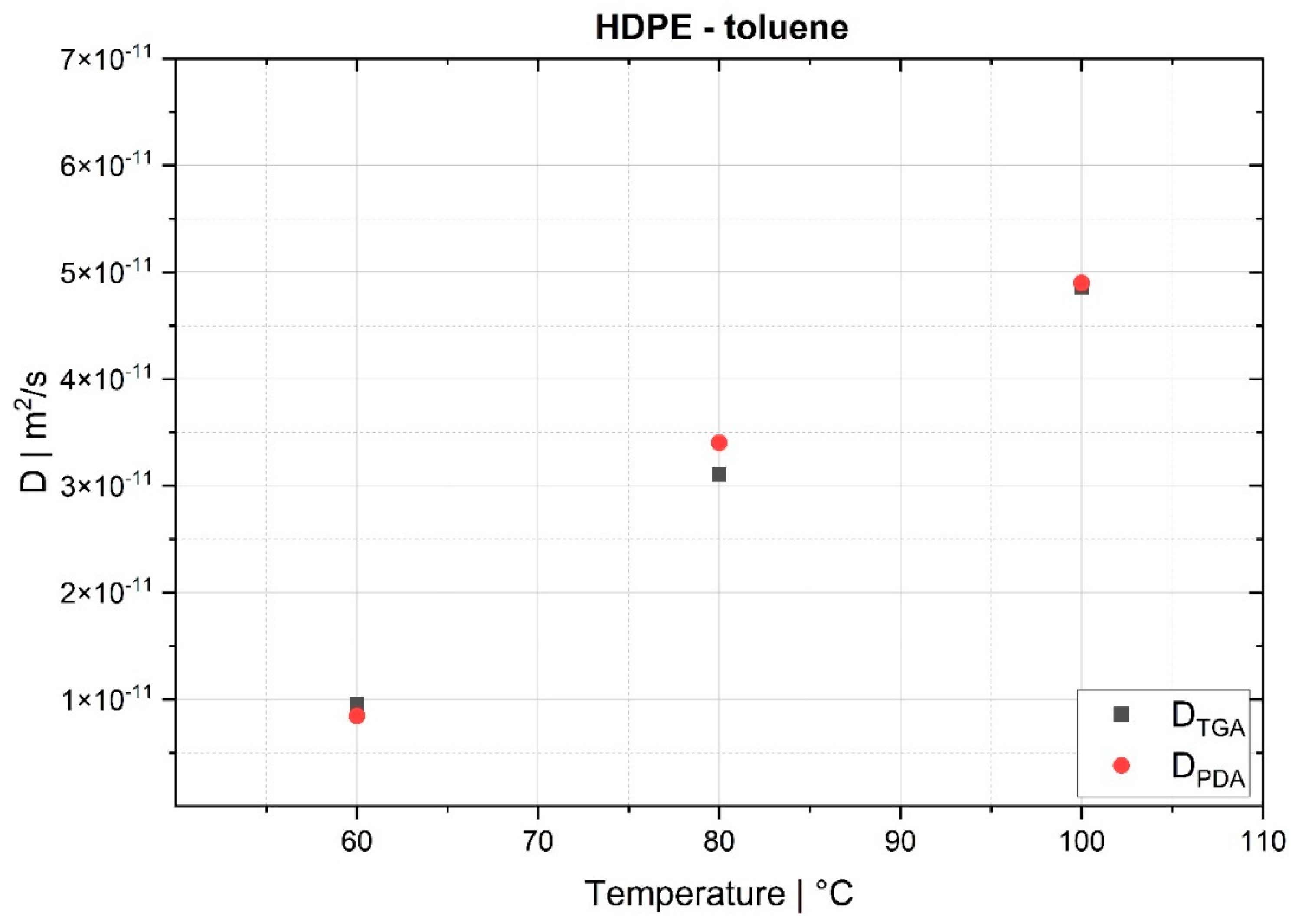
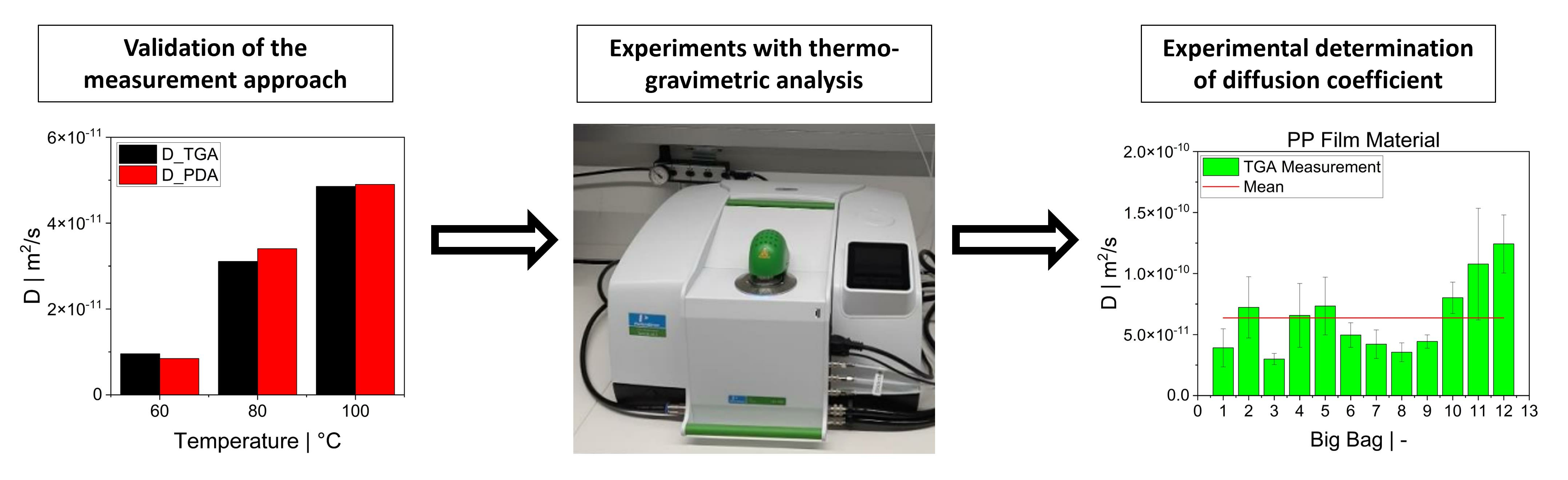
The focus of this study was on the assessment of a practically workable experimental method for evaluating diffusion coefficients under real process conditions. As the material feedstock in mechanical recycling usually exhibits some level of variation and contains unknown volatile substances, it is not possible to predict the diffusion coefficients for all binary mixtures involved. Therefore, our aim was to determine an “average” diffusion coefficient over all volatile substances at process temperatures. We present a feasible method using TGA to determine diffusion coefficients in the melt phase. 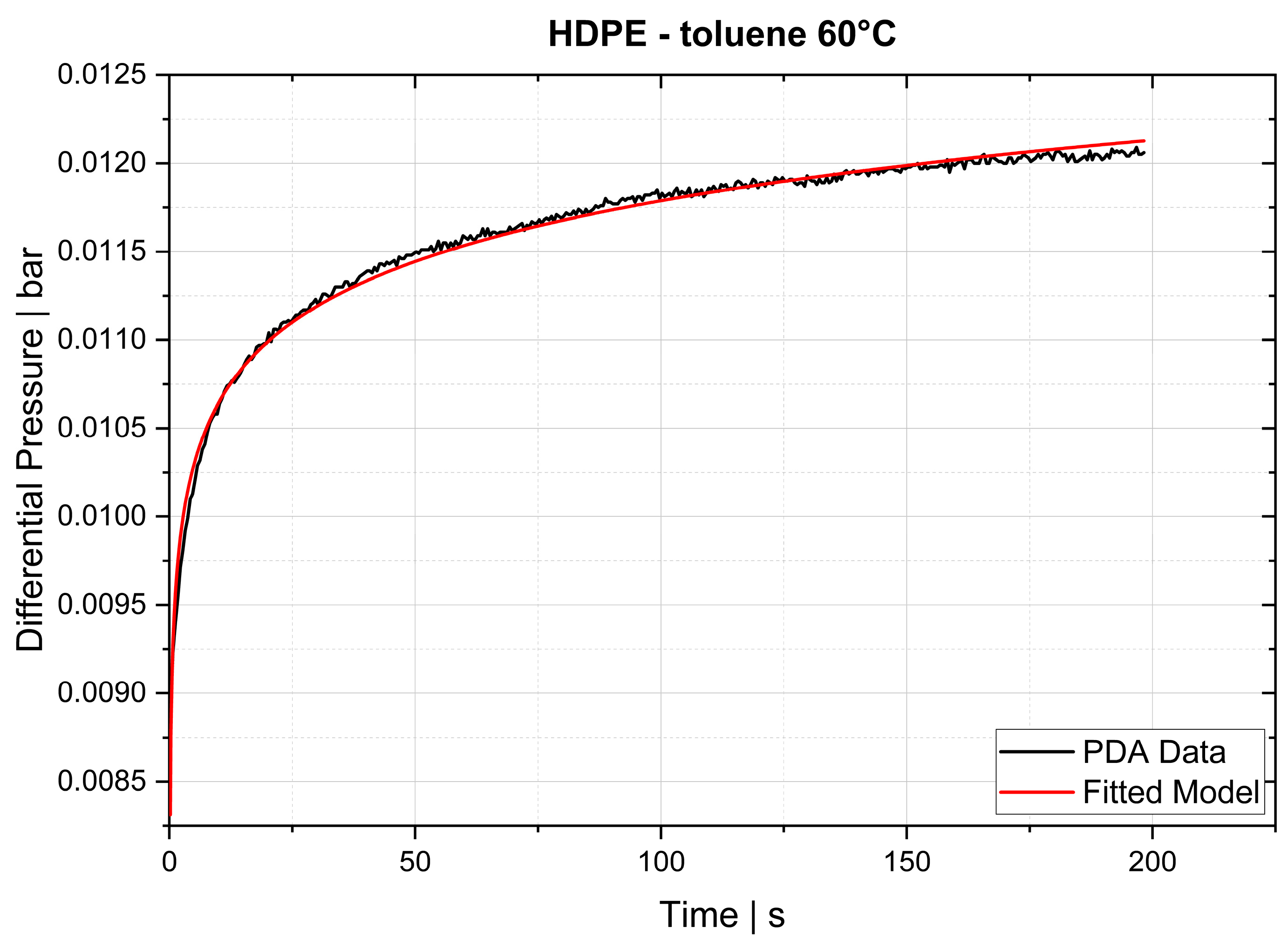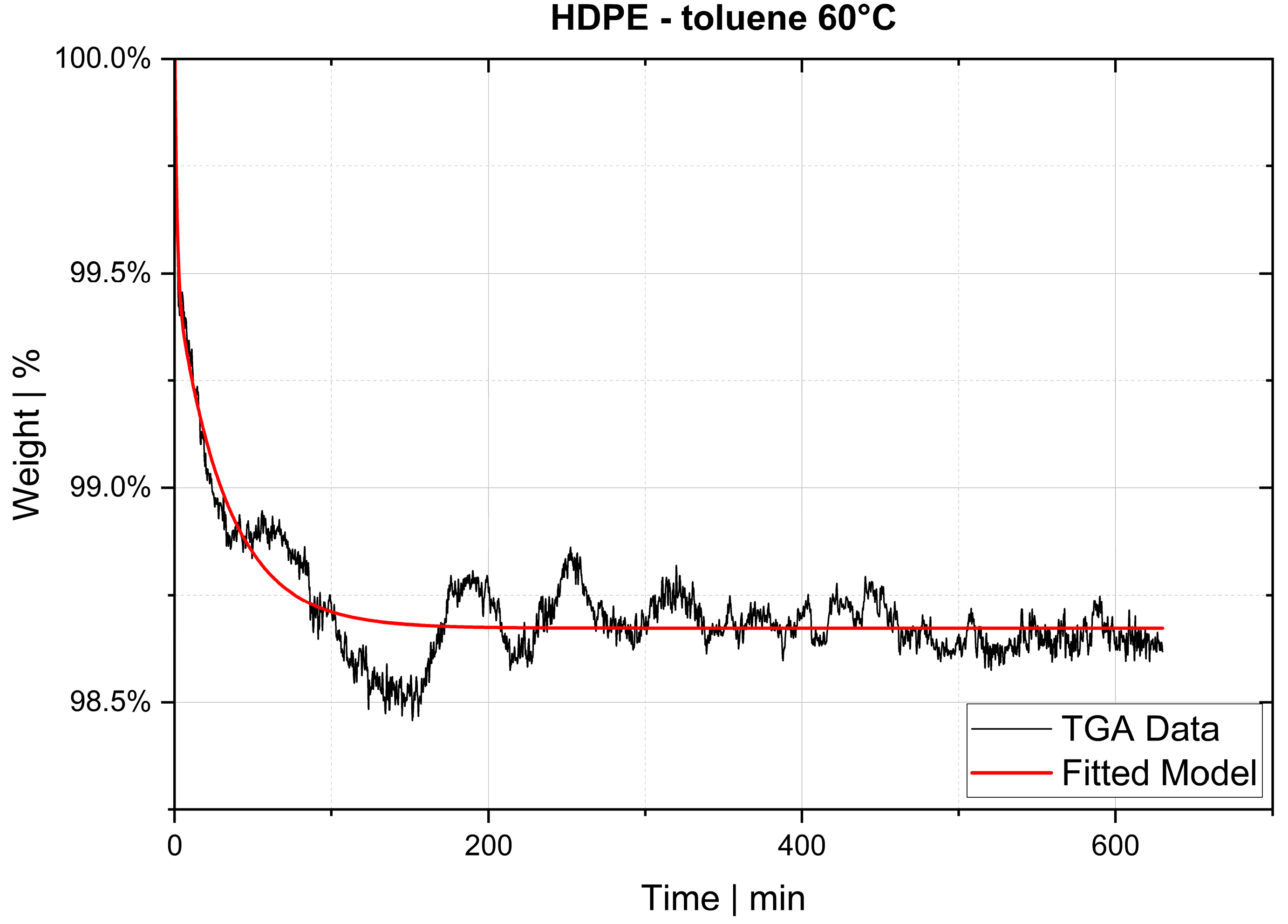Previous experimental studies on the measurement of diffusion coefficients sought to reproduce the literature values and/or were in most cases limited to a specific polymer/solvent system [23,24,25]. However, reproducing these experiments is difficult because the exact measurement conditions and the experimental procedure are in most cases poorly documented. Even the concentration of the substance in the sample depends on the test environment, as the equilibrium state is a function of, for instance, temperature and pressure. Rather than validating the TGA method by using the literature values, we took a different approach by applying a second experimental method. First, the TGA method was validated with experimental results obtained from a pressure decay apparatus (PDA). For this purpose, samples of high-density polyethylene (HDPE) and polypropylene (PP) were prepared and saturated with toluene. The same samples were used in both methods. The results of the PDA served as a reference value for the TGA. After successful validation, TGA was used to determine diffusion coefficients of post-industrial PP recyclates in the melt phase.

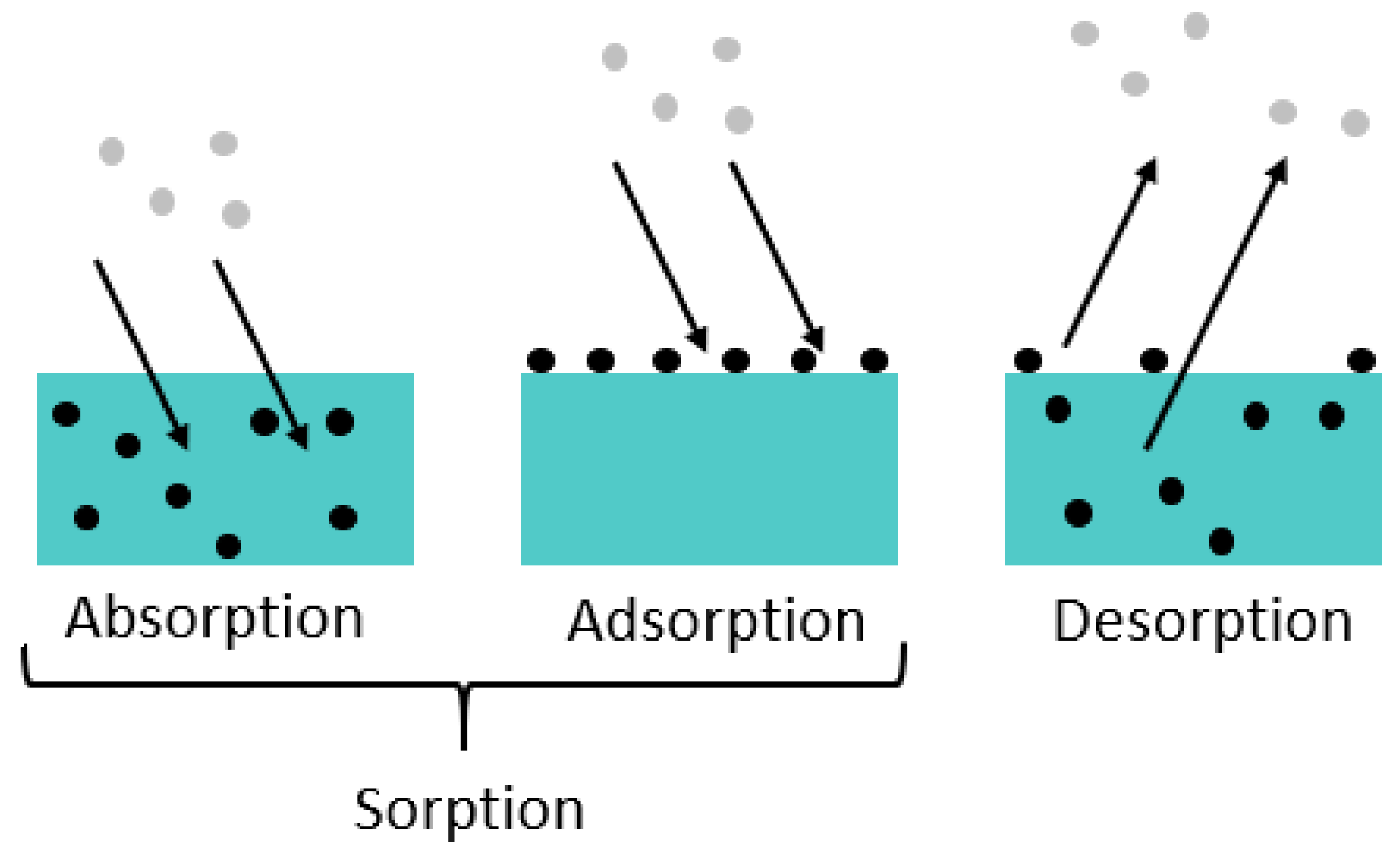
Diffusion is a physical process in which molecules of a substance become evenly distributed in a system. The Brownian motion causes the molecules to move from areas of higher concentration to areas of lower concentration. Three phenomena can be distinguished (see Figure 3 [26,27,28]): Sorption is a generic term and describes the accumulation of a particular substance in (i.e., absorption) or on (i.e., adsorption) another medium. Desorption is the reverse process, where the molecules of the dissolved substance leave, for example, the surface of a solid or the liquid in which they were dissolved.

2. Mathematical Background

Diffusion-based mass transport was described mathematically by Adolph Fick in 1855. He recognized analogies between diffusion and heat transfer by heat conduction. By adapting the equations of heat conduction, Fick established two relationships—still known today as Fick’s diffusion laws—that describe diffusion in isotropic materials [29]. To determine the diffusion coefficient, both methods we employed (TGA and PDA) use Fick’s second law, which describes the relationship between local and temporal changes in the concentration of a substance and states (see Equation (1)) that the dispersion of a gas or liquid is proportional to the spatial concentration gradient of that substance. The proportionality factor is called the diffusion coefficient (D) and is a measure of the velocity at which the substance is transported.

$$\frac{\mathit{\partial }c}{\mathit{\partial }t}=\frac{\mathit{\partial }}{\mathit{\partial }x}\left(D·\frac{\mathit{\partial }c}{\mathit{\partial }x}\right).$$

(1)

Solving Equation (1) strongly depends on the initial and boundary conditions [29]. If the initial concentration is $0$ or constant (i.e., $c=0$ or $c=c_0$) and the sample is symmetrical, then the boundaries can be defined as $x=0$ or $x=\pm l$. For a membrane, the following assumptions are made:

• In the area $-l<x<l$, there is a homogeneous initial concentration $c_0$, which means that $c=f\left(x\right)=c_0$.
• At the interfaces $x=\pm l$, the equilibrium concentration $c_2$ establishes spontaneously and prevails.
• The diffusion coefficient $D$ is constant, and is independent of the concentration in the sample ($D\ne D\left(c\right)$).

With these assumptions, Fick’s second diffusion law from Equation (1) results in the following trigonometric series:

$$\frac{c-c_0}{c_2-c_0}=1-\frac{4}{\pi }·\sum _{n=0}^{\infty }\frac{1^n}{2n+1}·\exp \left(\frac{-D·{\left(2n+1\right)}^2·{\pi }^2·t}{4·l^2}\right)·Cos\left(\frac{\left(2n+1\right)·\pi ·x}{2·l}\right).$$

(2)

If $M_t$ is the mass of substance diffused from the sample at time $t$ and $M_{\mathrm{\infty }}$ is the total mass of substance diffused from the sample at the thermodynamic equilibrium (steady state), the solution can be rewritten as:

$$\frac{M_t}{M_{\infty }}=1-\frac{8}{{\pi }^2}·\sum _{n=0}^{\infty }\frac{1}{{(2n+1)}^2}·\exp \left(\frac{-D·{\left(2n+1\right)}^2·{\pi }^2·t}{4·l^2}\right).$$

(3)

Since it is assumed that the diffusion coefficient is independent of concentration ($D\ne D\left(c\right)$), the mean value of the measurement is subsequently determined [29]. An analysis of TGA measurements requires making the following assumptions:

• A flat sample in the TGA crucible has only one diffusion surface; diffusion through the other surface is hindered by the bottom of the crucible. Although the symmetry of the sample as assumed in Equation (3) is thus no longer given, the solution can serve as a first approximation of the concentration profile when the total sample thickness is used, as suggested by Denson [23]. A more accurate treatment would involve solving Equation (1) with modified boundary conditions.
• The gas phase is initially free of diffusant.

3. Experimental

3.1. Pressure Decay Apparatus

The pressure decay method investigates the diffusion kinetics of a sample and records the pressure change over time at an isothermal temperature. As shown schematically in Figure 4, first the sample is heated to the desired temperature, and then the sample chamber is evacuated. The solvent, tempered in a separate chamber and brought into the gas phase, is introduced into the sample chamber to saturate the polymer sample. PDA allows for both sorption (saturation of a sample) and desorption (evaporation of volatiles from a sample) experiments to be carried out. In a sorption experiment, the solvent diffuses from the sample chamber into the sample over time. Consequently, both the concentration of the solvent in the sample chamber and the pressure decrease until a thermodynamic equilibrium is reached. In a desorption experiment, the solvent evaporates from the sample back into the sample chamber over time. Concentration and pressure in the sample chamber increase continuously until a steady state is reached. Figure 5 plots a desorption curve for a PDA experiment carried out with an HDPE-toluene system at a constant temperature of 60 °C. The diffusion coefficient, as shown in Equation (1), was fitted numerically from the entire measured curve shown in Figure 5. This gives different diffusion coefficients for individual measurements, from which a mean value is calculated as a material parameter.

3.2. Thermogravimetric Analysis

Without any modification to the instrument, TGA allows for only desorption tests to be performed. As with PDA, the diffusion kinetics of a sample over time at an isothermal temperature are investigated. A small circular sample was taken from saturated thin films. As shown in Figure 6, the sample was placed in the TGA crucible, and the sample chamber was purged with nitrogen as an inert gas. Over time, the solvent evaporated from the sample at an isothermal temperature. The resulting weight loss of the sample over time was recorded with a microbalance. The results of the pressure decay method served as benchmarks for validating the TGA method. The relationship between the two methods is as follows:

$$\frac{M_t}{M_{\infty }}=1-\frac{p_t}{p_{\infty }},$$

(4)

where $p_t$ is the pressure measured at time $t$ and $p_{\mathrm{\infty }}$ is the pressure at the steady state. The PDA experiment from Figure 5 was repeated with TGA. The desorption curve from the TGA measurement with the HDPE-toluene system at 60 °C is shown in Figure 7. Over time, the solvent diffuses out of the sample, decreasing the sample weight. This loss of weight over time is greatest at the beginning of the experiment because the difference in concentration is the greatest. The experiment continues until a thermodynamic equilibrium, and thus a steady state, is reached. In diffusion, the reaction processes occur in both directions. The solvent is also not distributed homogenously within the sample, which can lead to scattering in the measurement curve, as shown in Figure 7. As the system approaches equilibrium, the peaks and valleys converge.

To determine the diffusion coefficient from the TGA measurements, analogously to the PDA method, $D$ was fitted from the entire TGA curve using Equation (3), and the mean value was then calculated from multiple measurements.

3.3. Procedure for the Validation Study

For both the TGA and PDA measurements, thin sheets of HDPE and PP were pressed according to ISO 293:2004 standard [30] at 180 °C and 210 °C, respectively. The melt flow index (MFI) of the HDPE type was 4 g/10 min (test conditions: 190 °C and 2.16 kg) and the solid density was 954 kg/m³ [31], while the MFI of the PP type was 12 g/10 min (test conditions: 230 °C and 2.16 kg,) and the solid density was 908 kg/m³ [32]. Experiments were conducted with HDPE-toluene and PP-toluene systems using both TGA and PDA at temperatures of 60 °C, 80 °C and 100 °C to show the temperature dependence of the diffusion coefficient. For this purpose, the thin sheets with a thickness of approximately 150 μm (±5 μm) and dimensions of 58 mm × 108 mm were saturated with toluene in the PDA. The ambient pressure in the sample chamber during saturation (sorption experiment) was about 0.2 bar, which was approximately 60% of the vapor pressure of toluene. In the steady state, the excess toluene was evacuated from the sample chamber to subsequently investigate the dynamics of desorption diffusion. The diffusion coefficient from the PDA desorption experiments served as a reference value for the TGA experiments. For validation of the TGA method, all TGA measurements were carried out with the samples previously saturated in the PDA.

3.4. Procedure for Measuring Polymer Waste Materials

When successfully validated, TGA was used to experimentally determine the diffusion coefficient of various plastic waste materials at the processing temperature. This study shows the results of measuring post-industrial PP film material delivered in 12 big bags (approximately 10 tons in total). To consider the inhomogeneity of the feedstock and to obtain a statistically significant value, 3 TGA measurements per big bag (BB), and thus, a total of 36 measurements, were taken. Pre-shredding of the PP film material for the experiments resulted in flakes of various colors and sizes. Samples were taken from the BBs at three different positions: from the top, center and bottom of each BB [33]. These three samples were mixed and then crushed. The resulting “composite material” was used for the TGA measurements to ensure statistical validity. The diffusion coefficient in the polymer melt was determined at 220 °C, which is the barrel temperature in the degassing zone of an industrial extrusion process.

A strict interpretation of the method would require that all measurements be carried out until equilibrium is reached, when measurement values begin to plateau (steady state). In most measurements, this was not the case because the TGA experiments stopped after 20 h (1200 min). Since the slope of the curve is a measure of the diffusion coefficient and the curve is steepest at the beginning of each measurement, the contribution to the average diffusion coefficient is greatest at the beginning and smallest at the end of the experiment. To test whether ending the measurements before reaching the steady state affected the average diffusion coefficient measured, we simulated shortening the testing period for big bag 1 from 1200 min to 900 min. As can be seen in

Table 1. Comparison of the diffusion coefficients $D$ from 1200 min and 900 min measurements of samples from big bag 1.

Material	$\mathit{D}$1200 (TGA)|m2/s	$\mathit{D}$900 (TGA)|m2/s	$∆\mathit{D}$ (TGA)|m2/s
PP Film	2.963∙10−11	4.002∙10−11	1.039∙10−11
	2.660∙10−11	3.107∙10−11	4.463∙10−12
	6.112∙10−11	6.852∙10−11	7.404∙10−12

, reducing the measurement period caused only a small change—less than the scatter between measurements.

Since large variation in the feedstock material is to be expected when processing plastic waste, estimating the margin of error $m$ made with random samples from BBs is important. The equation for estimating the random sample size required is [34]:

$$n=\frac{\widehat{p}·(1-\widehat{p})·z^2}{m^2},$$

(5)

where $n$ is the sample size, $\widehat{p}$ is the proportion of the population, $z$ is the z-value for a given confidence interval (CI) and $m$ is the desired margin of error. The population is the entire set of flakes from which a statistical inference is to be drawn. Clearly, it is impossible to determine the diffusion coefficient for all flakes accumulated in the big bags. For this reason, a sufficiently large number of random samples must be taken to create a subset of the population that allows for conclusions to be drawn on the population with a specific degree of accuracy. The population proportion $\widehat{p}$ is in many cases—and was also in ours—unknown. For this reason, a “worst case” was assumed, and a value of $\widehat{p}$ = 0.5 was used. Since we sought to determine a diffusion coefficient for plastic waste, we did not choose the commonly used CIs of 0.99 or 0.95, but selected a value of 0.9. The corresponding $z$-value can be calculated or obtained from tables and is 1.28 for a CI of 0.9 [33]. Three measurements were carried out per BB. As a total of 12 BBs formed the population, we had a random sample size of $n$ = 36. Equation (5) can be transformed to obtain a margin of error $m$ of 0.11 for a mean value of D. The value of 0.11 corresponds to 11% and is close to the maximum value reported in the literature: According to Brase [34], the maximum value for the margin of error $m$ should be between 0.01 (1%) and 0.10 (10%). If the diffusion coefficients from the TGA measurements are normally distributed, then their mean value for any sample size $n$ is statistically representative. However, if this is not the case, the random sample size must be $n\ge$ 30 [34]. Although in this study the random sample size was 36, we took another 8 samples (11 in total) from big bag 1 to investigate more closely the scatter of measurements within a BB.

4. Results and Discussion

4.1. Validation Study

The experimental design for validating the TGA method, together with the results and the differences between TGA and PDA, is shown in

Table 2. Experimental validation of the diffusion coefficient D with data from TGA and the PDA.

System	Temp.|°C	$\mathit{D}$ (TGA)|m2/s	$\mathit{D}$ (PDA)|m2/s	$∆\mathit{D}$|m2/s
HDPE—toluene	60	9.565∙10−12	8.455∙10−12	1.110∙10−12
	80	3.105∙10−11	3.403∙10−11	2.979∙10−12
	100	4.856∙10−11	4.900∙10−11	4.366∙10−13
PP—toluene	60	9.732∙10−12	1.060∙10−11	8.679∙10−13
	80	1.670∙10−11	1.335∙10−11	3.353∙10−12
	100	5.259∙10−11	6.055∙10−11	7.958∙10−12

.

In the case of the HDPE-toluene system, both methods (TGA and PDA) gave similar results (see Table 2 and Figure 8). The diffusion coefficients for both techniques at 60 °C and 100 °C were almost identical. At 80 °C, the result from the TGA measurement was only marginally lower than that from the PDA. For the HDPE-toluene system, the diffusion coefficient exhibited an almost linear temperature dependence in the measurement range of 60–100 °C. Figure 9 shows the values for the diffusion coefficient of the PP toluene system from TGA and PDA tests at the same temperatures. Unlike for the HDPE-toluene system, a non-linear temperature relationship was observed using both methods, as exponentially higher $D$ values were obtained at 100 °C than at the other temperatures. Since the two approaches showed the same trend, both TGA and PDA were considered reliable. The different temperature dependencies for HDPE and PP might be explained by considering the morphological structure of the materials. For some polymers, tortuosity and the fraction of the amorphous phases can change with temperature and the presence of foreign substances. Therefore, the temperature relationship may be more pronounced at higher temperatures, which could explain the exponential slope.

4.2. Measurement of Polymer Waste Materials

The arithmetic mean of all TGA measurements of the post-industrial PP film material, together with standard deviation and standard error, can be seen in

Table 3. Mean value of the diffusion coefficients $D$ of all TGA measurements, including standard deviation SD and standard error SE.

Material	$\mathit{D}$mean (TGA)|m2/s	SD (TGA)|m2/s	SE (TGA)|m2/s
PP Film big bag 1	6.496∙10−11	2.243∙10−11	6.763∙10−12
(11 measurements)
PP Film total	6.367∙10−11	3.577∙10−11	5.962∙10−12
(36 measurements)

. The mean value of the TGA measurements across all BBs is almost identical to the mean value for big bag 1, and the standard deviations and standard errors also differ only slightly. Figure 10 and Figure 11 plot the results of the TGA measurements across all BBs and for big bag 1, respectively. Although the scatter of individual measurements, both within BB 1 and between BBs, is very high (see error bars), the mean values of the measurements are almost identical.

Figure A1 and Figure A2 in the Appendix A show an example TGA measurement for each BB, plotting both the TGA measurement curve and the corresponding curve fit. The values for the diffusion coefficient of the measurements over all BBs can be found in

Table A1. Values for diffusion coefficients $D$ from the TGA of PP film material (measured curve), including the mean value, standard deviation (SD) and concentration of volatile components C.

BB	$\mathit{D}$|m2/s	C|%	BB	$\mathit{D}$mean|m2/s	SD|m2/s
BB1-1	2.963·10−11	2.603
BB1-2	2.660·10−11	2.285	BB1	3.912·10−11	1.561·10−11
BB1-3	6.112·10−11	2.375
BB2-1	5.920·10−11	2.374
BB2-2	1.074·10−10	2.279	BB2	7.230·10−11	2.509·10−11
BB2-3	5.030·10−11	2.283
BB3-1	3.353·10−11	2.152
BB3-2	3.286·10−11	1.987	BB3	2.996·10−11	4.595·10−12
BB3-3	2.347·10−11	2.193
BB4-1	4.393·10−11	2.263
BB4-2	5.066·10−11	2.071	BB4	6.568·10−11	2.615·10−11
BB4-3	1.024·10−10	1.866
BB5-1	8.608·10−11	2.748
BB5-2	4.013·10−11	2.345	BB5	7.335·10−11	2.371·10−11
BB5-3	9.386·10−11	2.547
BB6-1	4.016·10−11	2.693
BB6-2	6.369·10−11	2.719	BB6	4.960$·$10−11	1.015·10−11
BB6-3	4.496·10−11	2.694
BB7-1	3.483·10−11	2.408
BB7-2	3.280·10−11	2.284	BB7	4.209·10−11	1.173·10−11
BB7-3	5.864·10−11	2.394
BB8-1	2.899·10−11	2.181
BB8-2	3.109·10−11	2.365	BB8	3.549·10−11	7.757·10−12
BB8-3	4.639·10−11	1.942
BB9-1	3.850·10−11	2.035
BB9-2	5.154·10−11	2.396	BB9	4.432·10−11	5.417·10−12
BB9-3	4.291·10−11	2.230
BB10-1	7.878·10−11	2.322
BB10-2	6.513·10−11	2.303	BB10	8.017·10−11	1.288·10−11
BB10-3	9.659·10−11	2.205
BB11-1	1.695·10−10	1.800
BB11-2	9.395·10−11	2.441	BB11	1.077·10−10	4.583·10−11
BB11-3	5.976·10−11	1.998
BB12-1	9.998·10−11	2.174
BB12-2	1.566·10−10	2.077	BB12	1.242·10−10	2.383·10−11
BB12-3	1.161·10−10	2.207

(Appendix A), and those for big bag 1 in

Table A3. Diffusion coefficients $D$ from the TGA of PP film material from big bag 1 (measured curve), including the mean value, standard deviation (SD) and concentration of volatile components C.

BB	$\mathit{D}$|m2/s	C|%	BB	$\mathit{D}$mean|m2/s	SD|m2/s
BB1-1	2.963∙10−11	2.603	BB1	6.496∙10−11	2.243∙10−11
BB1-2	2.660∙10−11	2.285
BB1-3	6.112∙10−11	2.375
BB1-4	7.567∙10−11	2.383
BB1-5	6.776∙10−11	2.579
BB1-6	5.634∙10−11	2.650
BB1-7	9.511∙10−11	2.485
BB1-8	7.701∙10−11	2.599
BB1-9	9.719∙10−11	2.458
BB1-10	6.563∙10−11	2.564
BB1-11	6.246∙10−11	2.662

(Appendix A). The diffusion coefficient characteristics were determined using the original, measured and not the fitted values. The diffusion coefficients calculated for the curve fittings are given in

Table A2. Diffusion coefficients $D$ from the TGA of PP film material (curve fit), including the mean value, standard deviation (SD) and concentration of volatile components C.

BB	$\mathit{D}$|m2/s	C|%	BB	$\mathit{D}$mean|m2/s	SD|m2/s
BB1-1	3.400·10−11	2.507
BB1-2	3.049·10−11	2.219	BB1	4.449·10−11	1.737·10−11
BB1-3	6.897·10−11	2.328
BB2-1	6.600·10−11	2.336
BB2-2	1.174·10−10	2.264	BB2	7.987·10−11	2.682·10−11
BB2-3	5.623·10−11	2.259
BB3-1	3.893·10−11	2.078
BB3-2	3.684·10−11	1.961	BB3	3.408·10−11	5.448·10−12
BB3-3	2.647·10−11	2.144
BB4-1	4.748·10−11	2.246
BB4-2	5.490·10−11	2.057	BB4	6.990·10−11	2.664·10−11
BB4-3	1.073·10−10	1.881
BB5-1	6.039·10−11	2.905
BB5-2	4.206·10−11	2.323	BB5	5.261·10−11	7.733·10−12
BB5-3	5.538·10−11	2.614
BB6-1	4.400·10−11	2.679
BB6-2	7.436·10−11	2.632	BB6	5.601·10−11	1.318·10−11
BB6-3	4.965·10−11	2.668
BB7-1	3.935·10−11	2.354
BB7-2	3.981·10−11	2.161	BB7	4.781·10−11	1.164·10−11
BB7-3	6.427·10−11	2.376
BB8-1	3.167·10−11	2.158
BB8-2	3.707·10−11	2.274	BB8	3.989·10−11	8.107·10−12
BB8-3	5.092·10−11	1.910
BB9-1	3.859·10−11	2.075
BB9-2	5.150·10−11	2.452	BB9	4.505·10−11	5.271·10−12
BB9-3	4.505·10−11	2.217
BB10-1	8.908·10−11	2.277
BB10-2	5.622·10−11	2.403	BB10	8.230·10−11	1.914·10−11
BB10-3	1.016·10−10	2.203
BB11-1	1.994·10−10	1.774
BB11-2	1.072·10−10	2.346	BB11	1.239·10−10	5.605·10−11
BB11-3	6.517·10−11	1.993
BB12-1	1.135·10−10	2.130
BB12-2	1.689·10−10	2.068	BB12	1.363·10−10	2.362·10−11
BB12-3	1.266·10−10	2.187

and

Table A4. Diffusion coefficients $D$ from the TGA of PP film material from big bag 1 (curve fit), including the mean value, standard deviation (SD) and concentration of volatile components C.

BB	$\mathit{D}$|m2/s	C|%	BB	$\mathit{D}$mean|m2/s	SD|m2/s
BB1-1	3.400∙10−11	2.507	BB1	8.347∙10−11	5.372∙10−11
BB1-2	3.049∙10−11	2.219
BB1-3	6.897∙10−11	2.328
BB1-4	8.333∙10−11	2.363
BB1-5	7.400∙10−11	2.563
BB1-6	6.052∙10−11	2.641
BB1-7	2.311∙10−10	1.734
BB1-8	8.561∙10−11	2.566
BB1-9	1.088∙10−10	2.426
BB1-10	7.191∙10−11	2.544
BB1-11	6.939∙10−11	2.626

(Appendix A). The difference between the diffusion coefficients from the original measurement curve and from the fitted curve is in most cases smaller than the scattering between the individual measurements. Interestingly, the values for the diffusion coefficient are almost consistently higher for the fitted curves. The fits result in values that are too high (higher than those measured), especially at the beginning of each measurement. However, it is precisely this early phase that is critical to determining the diffusion coefficient. For this reason, all calculations for the experimental determination of the diffusion coefficient used the original TGA measurement curves and not the fitted curves. With a few exceptions, the concentrations of the volatile components are clearly above 2% and are close together. Overall, considering that material from plastic waste was used, the measurement results are very satisfactory. The results from desorption tests always exhibit a high degree of scattering, as foreign substances are usually not homogeneously distributed in the material.

5. Summary and Conclusions

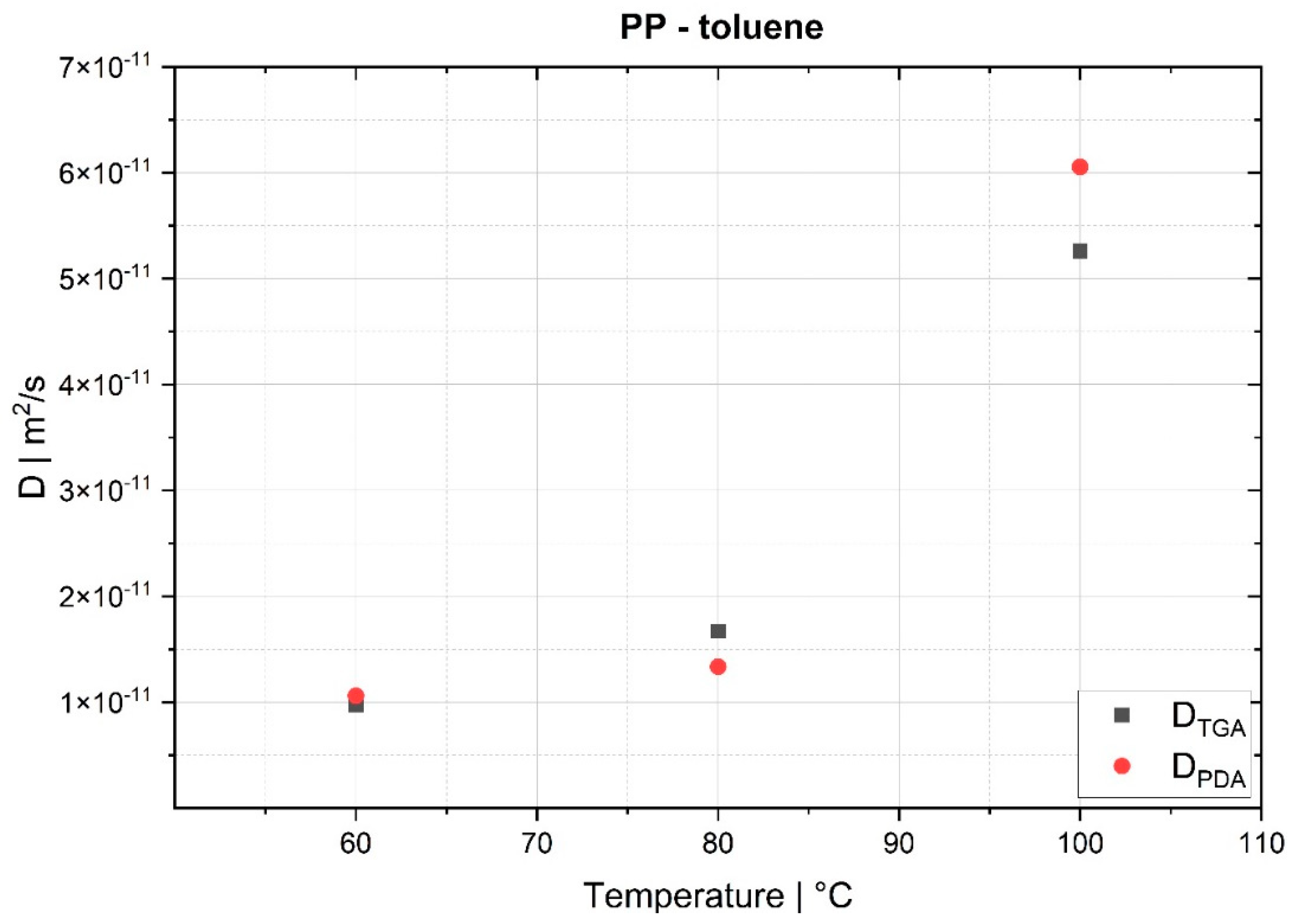
The desorption experiments in this study show that thermogravimetric analysis (TGA) offers a practical way to determine the diffusion coefficient experimentally. To validate the TGA method, both pressure decay apparatus tests and thermogravimetric analyses were performed at 60 °C, 80 °C and 100 °C. The two techniques yielded comparable results, with an average difference of 7.4% for the HDPE-toluene system and 14.7% for the PP-toluene system. Thus, TGA has potential for use in determining the diffusion coefficient in desorption experiments. The selection of a suitable method depends on many factors (e.g., application, material, and availability); in principle, both methods are suited for determining $D$, but each method has its own advantages.

On the one hand, the great advantages of the pressure decay method are (i) that it delivers results very quickly, as the measurements take only a few minutes, and (ii) that it allows for both sorption and desorption experiments to be carried out. TGA, on the other hand, offers the advantage of being an almost universal measuring technique and thus widely used in laboratories and research institutions, rendering the acquisition of new equipment unnecessary in most cases. TGA devices are easy to operate, and the amount of work per measurement is low. Further, as demonstrated, the method shows potential for determining $D$ in the melt under process conditions. However, TGA allows for only desorption tests to be performed, and measurements take several hours, which is a considerable disadvantage compared to the pressure decay method.

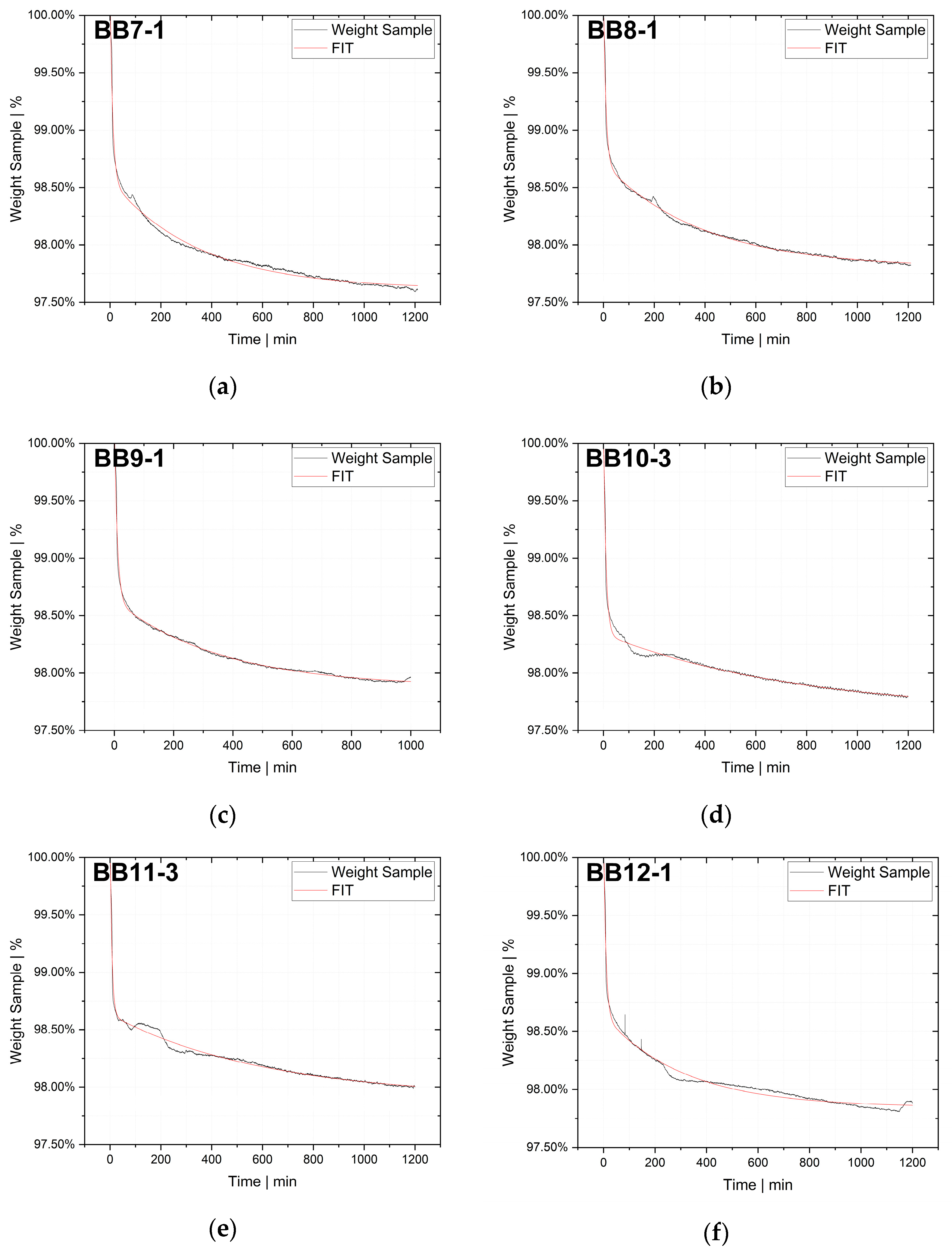
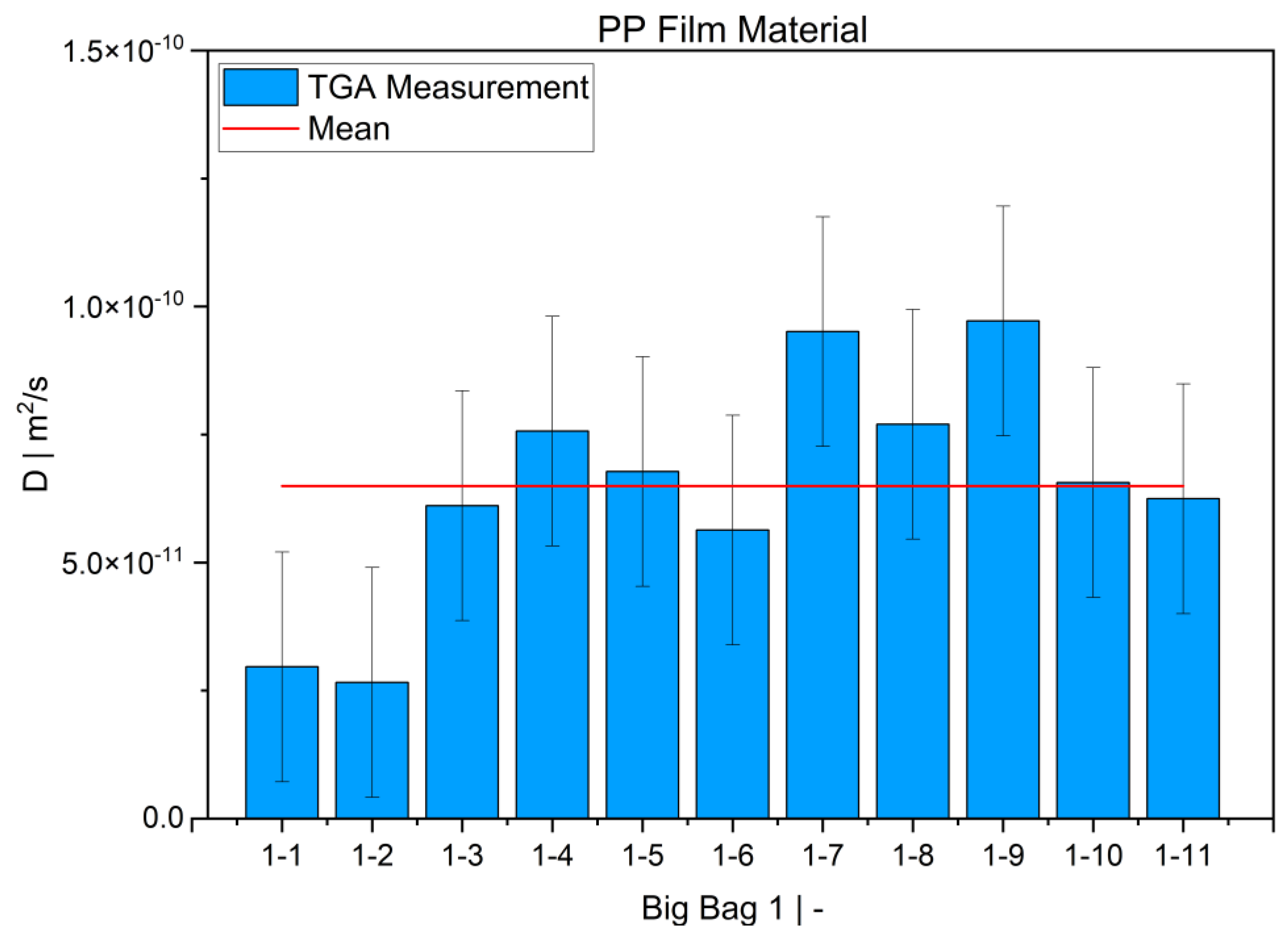
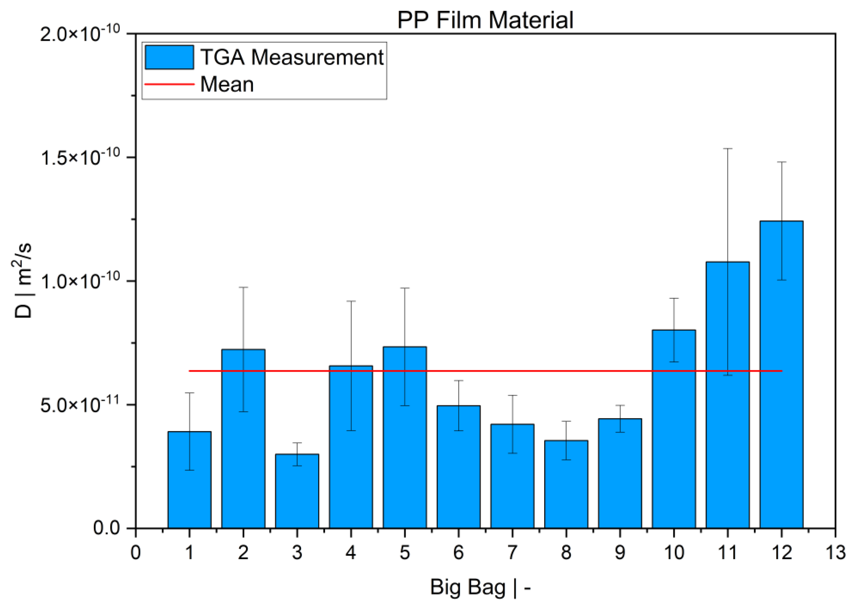
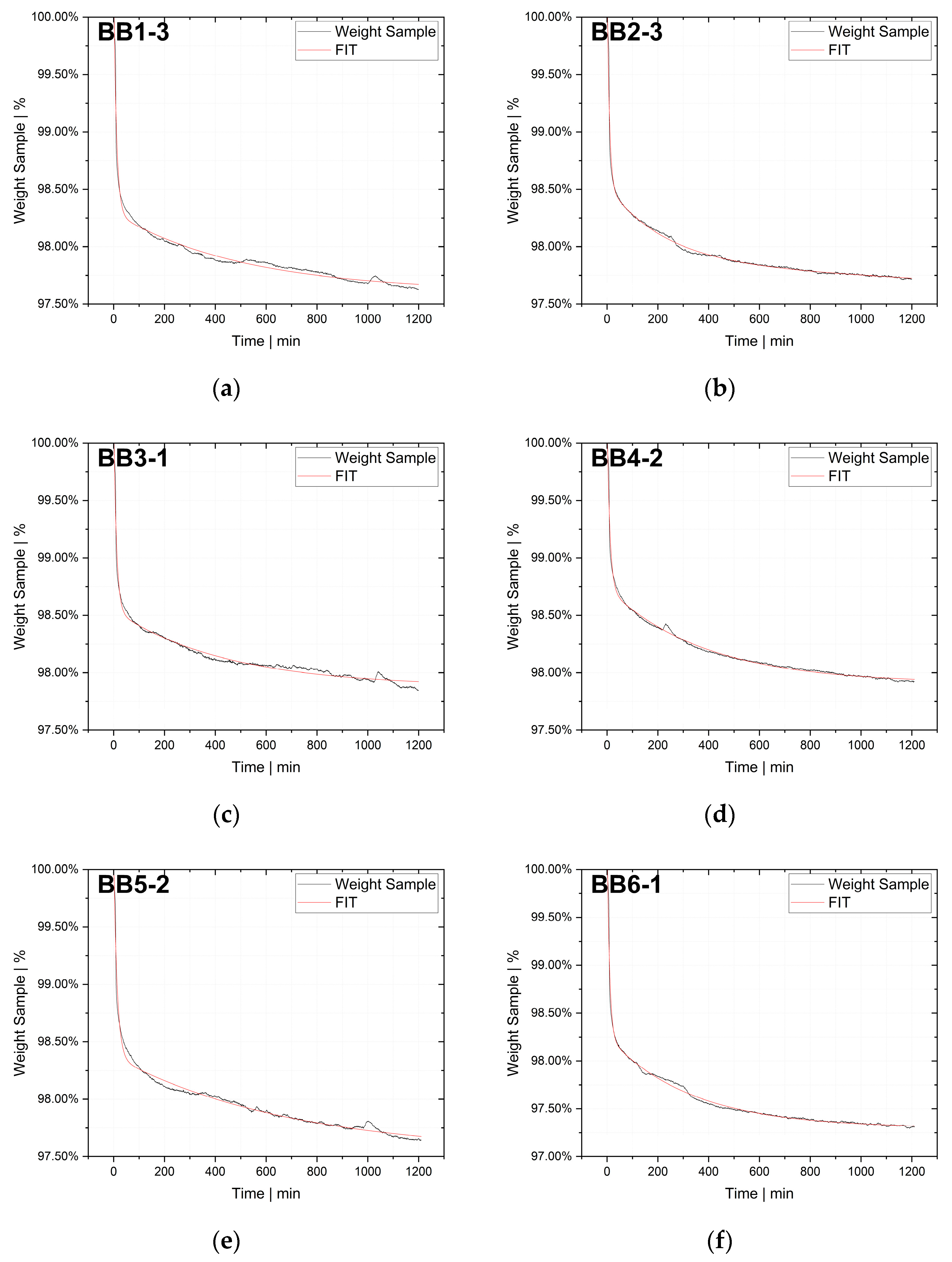
TGA was used in this study to determine the diffusion coefficient in the melt of plastic waste material at 220 °C. Care was taken to ensure that the measurements were statistically representative. All 12 big bags contributed material to the 36 TGA measurements carried out, from which the mean value was then determined. Overall, the standard deviations were low, thus indicating the reproducibility of the measurements. For big bag 1, 8 additional measurements (11 measurements in total) were taken to confirm the normal distribution of the TGA measurements in one big bag.

References

1. Plastics Europe. Plastics—The Facts 2022; Plastics Europe AISBL: Brussels, Belgium, 2022. [Google Scholar]
2. European Parliament. Directive 2008/98/EC on Waste and Repealing Certain Directives; European Union: Brussels, Belgium, 2018. [Google Scholar]
3. Badini, C.; Ostrovskaya, O.; Bernagozzi, G.; Lanfranco, R.; Miranda, S. Recycling of Polypropylene Recovered from a Composting Plant: Mechanical Behavior of Compounds with Virgin Plastic. Recycling 2023, 8, 62. [Google Scholar] [CrossRef]
4. Open Access Government. EU Green Deal: Creating a Circular Economy for Plastics. Available online: https://www.openaccessgovernment.org/circular-economy-for-plastics/97160/ (accessed on 25 March 2023).
5. European Commission. Fit for 55: Delivering the EU’s 2030 Climate Target on the Way to Climate Neutrality; European Commission: Brussels, Belgium, 2021. [Google Scholar]
6. Costa, A.A.; Martinho, P.G.; Barreiros, F.M. Comparison between the Mechanical Recycling Behaviour of Amorphous and Semicrystalline Polymers: A Case Study. Recycling 2023, 8, 12. [Google Scholar] [CrossRef]
7. Francis, R. Recycling of Polymers: Methods, Characterization and Applications; Wiley-VCH: Weinheim, Germany, 2016; ISBN 978-3-527-33848-1. [Google Scholar]
8. Hopewell, J.; Dvorak, R.; Kosior, E. Plastics recycling: Challenges and opportunities. Philos. Trans. R. Soc. B Biol. Sci. 2009, 364, 2115–2126. [Google Scholar] [CrossRef] [PubMed]
9. Ragaert, K.; Delva, L.; Geem, K.V. Mechanical and chemical recycling of solid plastic waste. Waste Manag. 2017, 69, 24–58. [Google Scholar] [CrossRef]
10. McKinlay, R. Sorting Requirements—PlastiCircle; PlastiCircle—Grant Agreement 730292; UK, 2018; Available online: https://plasticircle.eu/fileadmin/user_upload/PlastiCircle_D4.1_FINAL_PU_M10.pdf (accessed on 15 June 2023).
11. Schyns, Z.O.G.; Shaver, M.P. Mechanical Recycling of Packaging Plastics: A Review. Macromol. Rapid Commun. 2020, 42, 2000415. [Google Scholar] [CrossRef] [PubMed]
12. La Mantia, F.P. Basic Concepts on the Recycling of Homogeneous and Heterogeneous Plastics; Recycling of PVC and Mixed Plastic Waste; ChemTec Publishing: Scarborough, ON, Canada, 1996; ISBN 9781895198119. [Google Scholar]
13. Karpfer, K. Entgasen in der Kunststoffaufbereitungstechnik. Vak. Prax. 1993, 5, 15–22. [Google Scholar] [CrossRef]
14. Albalak, R.J. An Introduction to Devolatilization in Polymer Devolatilization; Marcel Dekker Inc.: New York, NY, USA, 1996; pp. 1–12. ISBN 0-8247-9627-6. [Google Scholar]
15. Hirschfeld, S.; Wuensch, O. Bubble-Free Polymer Devolatilization in a Simplified Extruder Model; AIP Publishing LLC: Melville, NY, USA, 2019. [Google Scholar] [CrossRef]
16. Gestring, I. Entgasen von Polymeren. Ph.D. Thesis, University of Hannover, Welfengarten, Germany, 2002. [Google Scholar]
17. Wang, N.H. Comparison between surface renewal devolatilizing performances of different screw extruders. Soc. Plast. Eng. 2007, 47, 1920–1926. [Google Scholar] [CrossRef]
18. Biesenberger, J.A. Entgasung von Kunststoffen in Scherströmungsfeldern; VDI Gesellschaft Kunststofftechnik: Duesseldorf, Germany, 1993; ISBN 3-18-401274-3. [Google Scholar]
19. Czeslik, C.; Seemann, H.; Winter, R. Basiswissen Physikalische Chemie—2. Auflage; Teubner Verlag: Berlin/Heidelberg, Germany, 2007; ISBN 978-3-8351-0047-3. [Google Scholar]
20. Job, G.; Rüffler, R. Physikalische Chemie—Eine Einführung nach Neuem Konzept mit Zahlreichen Experimenten; Vieweg + Teubner Verlag: Berlin/Heidelberg, Germany, 2011; ISBN 978-3-8351-0040-4. [Google Scholar]
21. Cussler, E.L. Diffusion—Mass Transfer in Fluid Systems; Cambridge University Press: Cambridge, UK, 2007; ISBN 978-0-511-47892-5. [Google Scholar]
22. Bakker, H.; Bonzel, H.P.; Bruff, C.M.; Dayananda, M.A.; Gust, W.; Horvath, J.; Kaur, I.; Kidson, G.V.; Le Claire, A.D.; Mehrer, H.; et al. Numerical Data and Functional Relationships in Science and Technology; Diffusion in Solid Metals and Alloys; Springer: Berlin/Heidelberg, Germany, 1990; ISBN 978-3-540-46109-8. [Google Scholar]
23. Denson, C.D. Measurement of Diffusion Coefficient of Organic Volatile Components in Polymer Melts; SPE Extrusion Division: Danbury, CT, USA, 1989. [Google Scholar]
24. Igwe, I.O.; Ewulonu, C.M.; Igboanugo, I. Studies on the Diffusion Characteristics of some Aromatic Solvents into Polypropylene Film. J. Appl. Polym. Sci. 2006, 102, 1985–1989. [Google Scholar] [CrossRef]
25. Prasad, T.V.; Brown, K.W.; Thomas, J.C. Diffusion coefficient of organics in high density polyethylene (HDPE). Waste Manag. Res. 1994, 12, 61–71. [Google Scholar] [CrossRef]
26. Grathwohl, P. Diffusion in Natural Porous Media: Contaminant Transport, Sorption/Desorption and Dissolution Kinetics; Springer Science and Business Media LLC: Berlin/Heidelberg, Germany, 1998; ISBN 978-1-4613-7602-6. [Google Scholar]
27. Rachinskii, V.V. The General Theory of Sorption Dynamics and Chromatography; Consultants Bureau: New York, NY, USA, 1965; ISBN 978-1-4757-0063-3. [Google Scholar]
28. Wutz, M.; Adam, H.; Walcher, W. Theorie und Praxis der Vakkumtechnik 5. Auflage; Vieweg Verlag: Wiesbaden, Germany, 1992; ISBN 978-3-528-34884-7. [Google Scholar]
29. Crank, J. The Mathematics of Diffusion, 2nd ed.; Clarendon Press: Oxford, UK, 1975; ISBN 0-19-853344-6. [Google Scholar]
30. ISO 293:2004; Plastics—Compression Moulding of Test Specimens of Thermoplastic Materials. 2004. Available online: https://www.iso.org/standard/39885.html (accessed on 15 June 2023).
31. Product Data Sheet. Polyethylene BorePure MB7541; Borealis AG: Vienna, Austria, 2018. [Google Scholar]
32. Product Data Sheet. Polypropylene HE125MO; Borealis AG: Vienna, Austria, 2007. [Google Scholar]
33. Akhras, M.H.; Fischer, J. Sampling Scheme Conception for Pretreated Polyolefin Waste Based on a Review of the Available Standard Procedures. Polymers 2022, 14, 3450. [Google Scholar] [CrossRef] [PubMed]
34. Brase, C.H.; Brase, C.P. Understanding Basic Statistics, 7th ed.; Cengage Learning: Boston, MA, USA, 2014; ISBN 978-1-305-25406-0. [Google Scholar]
Figure 1. Material stream in the life cycle of plastics.
Recycling 08 00072 g001
Figure 2. Overview of a mechanical recycling process.
Recycling 08 00072 g002
Figure 3. Schematics of sorption and desorption processes.
Recycling 08 00072 g003
Figure 4. Schematic illustration of PDA (source: http://www.kosekgroup.cz/equipment/pressure-decay-apparatus/ accessed on 18 February 2023).
Recycling 08 00072 g004
Figure 5. PDA desorption experiment using an HDPE-toluene system at 60 °C.
Recycling 08 00072 g005
Figure 6. Schematic illustration of TGA.
Recycling 08 00072 g006
Figure 7. TGA desorption experiment using an HDPE-toluene system at 60 °C.
Recycling 08 00072 g007
Figure 8. Comparison of the TGA and PDA results for the HDPE-toluene system.
Recycling 08 00072 g008
Figure 9. Comparison of the TGA and the PDA results for the PP-toluene system.
Recycling 08 00072 g009
Figure 10. Mean value of the diffusion coefficient for each BB (bars), mean value for all BBs (red line) and standard deviation per BB as the error bar.
Recycling 08 00072 g010
Figure 11. Mean value of the diffusion coefficient for BB 1 (bars), mean value over all measurements (red line) and standard deviation as the error bars.
Recycling 08 00072 g011