Abstract
This work contributes to the recycling of technical black plastic particles, for example from the automotive or electronics industries. These plastics cannot yet be sorted with sufficient purity (up to 99.9%), which often makes economical recycling impossible. As a solution to this problem, imaging fluorescence spectroscopy with additional illumination in the near infrared spectral range in combination with classification by machine learning or deep learning classification algorithms is here investigated. The algorithms used are linear discriminant analysis (LDA), k-nearest neighbour classification (kNN), support vector machines (SVM), ensemble models with decision trees (ENSEMBLE), and convolutional neural networks (CNNs). The CNNs in particular attempt to increase overall classification accuracy by taking into account the shape of the plastic particles. In addition, the automatic optimization of the hyperparameters of the classification algorithms by the random search algorithm was investigated. The aim was to increase the accuracy of the classification models. About 400 particles each of 14 plastics from 12 plastic classes were examined. An attempt was made to train an overall model for the classification of all 12 plastics. The CNNs achieved the highest overall classification accuracy with 93.5%. Another attempt was made to classify 41 mixtures of industrially relevant plastics with a maximum of three plastic classes per mixture. The same average classification accuracy of 99.0% was achieved for the ENSEMBLE, SVM, and CNN algorithms. The target overall classification accuracy of 99.9% was achieved for 18 of the 41 compounds. The results show that the method presented is a promising approach for sorting black technical plastic waste.
1. Introduction
The material recycling of raw materials is of growing importance in view of finite resources, rising demand, and environmentally damaging extraction and production conditions. This applies in particular to plastics, which are currently manufactured largely from crude oil. The rate of material recycling of plastics worldwide is currently only around 9%. A further 11% is used for thermal recycling, while the remainder is landfilled [1]. The majority of recycled plastics are also often processed into inferior secondary products. The reason for this is the lack of suitable sensor technologies for classifying plastics, which makes it possible to separate plastic mixtures with sufficient purity (sometimes up to 99.9%). This applies in particular to technical black plastics, which often consist of a complex material mix and are coloured black by carbon fillers. The standard separation technologies used for sorting plastics, such as classification using float-sink methods [2] or electrostatic separation [3] or sorting using hyperspectral imaging (HSI) in the near-infrared spectral range [4,5], are not suitable for black plastics. Other methods such as X-ray fluorescence (XRF) [6] are suitable for sorting black plastics but are limited to a small number of plastic combinations.
For the sorting of technical black plastics, some approaches are currently being developed, and some are already being offered commercially. These include hyperspectral imaging in the mid-infrared spectral range [7,8] and terahertz spectroscopy [9,10]. Both approaches allow the sorting of black plastics but are not optimal due to expensive instrument technology, low achievable throughputs, and large required particle sizes. Another possibility is the use of laser-induced breakdown spectroscopy (LIBS) or Raman spectroscopy [11,12]. However, both approaches are not yet widely used in industrial applications for sorting black plastics.
The most promising technology at present is the classification of black plastics on the basis of their fluorescence. Many plastics show a characteristic fluorescence if they are illuminated with intensive laser radiation. The exact causes of fluorescence are not well studied. It is assumed that fluorescence is mainly caused by additives or impurities in the plastics [13,14,15]. With this technology, it is also possible to classify black plastics, and there has already been commercial implementation. The achieved accuracies do not exceed 98% [16].
The aim of this work is to improve the technology of fluorescence spectroscopy for the sorting of black plastics and thus to further increase the classification accuracy. For this purpose, fluorescence spectroscopy is to be combined with hyperspectral imaging. In this way, in addition to the fluorescence spectra of the plastic particles, their shape and texture are also obtained. This is especially characteristic for the type of plastic for particles generated by cryogenic grinding [17]. Convolutional Neural Networks (CNNs), which have achieved great success in the classification of image data, will be used to consider the shape of the plastic particles in the classification [18,19,20].
For the experiments, about 400 particles each of 14 black plastics in 12 plastic classes were measured with an imaging fluorescence spectrometer. The particles were produced by cryogenic grinding and range in size from 5 mm to 12 mm. The data obtained was then used to train various machine learning algorithms and compare them using statistic methods. The ‘classical’ machine learning algorithms linear discriminant analysis (LDA [21]), k-nearest neighbour classification (kNN [22]), support vector machines (SVM [23]), and ensemble models with decision trees (ENSEMBLE [24]) were trained. The particle shape was not considered for these algorithms. Convolutional neural networks were trained considering the particle shape [18]. Therefore, spectral images of the particles were generated, which show the particle shape as well as their fluorescence properties. For plastics without fluorescence, reflectivity in the near-infrared spectral range (NIR) was used to detect the position and shape of the particles. For all trained algorithms, an automatic hyperparameter optimization by random search (RS, [25]) was performed. The aim was to increase the achievable overall classification accuracy of the models. The hyperparameter optimization by BOA was also tried but did not provide better results than RS and is therefore not shown for reasons of clarity. At the same time, an automated optimization of the hyperparameters of the classification algorithms allows for a simple training of models for the classification of new plastics. This reduces the demands placed on plant operators during subsequent industrial use, since the user does not need to have any prior knowledge of machine learning. The obtained classification accuracies of the models were examined by means of ANOVA with subsequent Tukey test with regard to statistically significant differences. Models for the simultaneous classification of all 12 plastic classes and for the classification of 41 industrially relevant mixtures of two to three plastic classes were examined.
It was found that CNNs using the spectral and shape information can achieve statistically significantly and better overall classification accuracy for the classification of all 12 plastics than classical machine learning algorithms using only the spectral information. For the classification of the mixtures, there were no differences between the three considered algorithms—ENSEMBLE, SVM, and CNN. Furthermore, the automatic optimization of the hyperparameters by random optimization proved to be a very good possibility to improve the overall classification accuracy of the models. In total, the desired overall classification accuracy of 99.9% could be achieved for 18 of the 41 plastic mixtures with two or three classes.
2. Materials and Methods
2.1. Description of the Used Black Plastics
For the experiments carried out, 14 different black plastics in 12 plastic classes were used. The sales description and the manufacturer of the plastic samples are not known. The following types of plastics have been investigated:
- high-density polyethylene (HDPE, 399 particles);
- polypropylene (PP, 399 particles);
- polyoxymethylene (POM, 399 particles);
- polyphenylene sulfide (PPS, 400 particles);
- polyamide 6 and polyamide 6 (PA6) with glass fibre /without glass fibre (798 particles);
- polyamide 66 and polyamide 66 (PA66) with glass fibre /without glass fibre (756 particles);
- polyamide 66 with flame retardant (PA66 V0, 396 particles);
- styrene-butadiene rubber (SBR, 390 particles);
- polybutylene terephthalate (PBT, 399 particles);
- thermoplastic elastomers (TPE, 397 particles);
- thermoplastic polyurethanes (TPU, 392 particles);
- thermoplastic copolyester (TEEE, 402 particles).
The numbers show the amount of particles measured per polymer. The samples of the polymers were obtained from a recycling company and crushed to a grain size of 5 mm to 12 mm by cryogenic grinding before examination [17]. The polyamides (PA6 and PA66) were measured with and without glass fibres as additional filler. For the evaluation, plastics with and without glass fibres were considered as one class.
2.2. Imaging Fluorescence Spectrometer
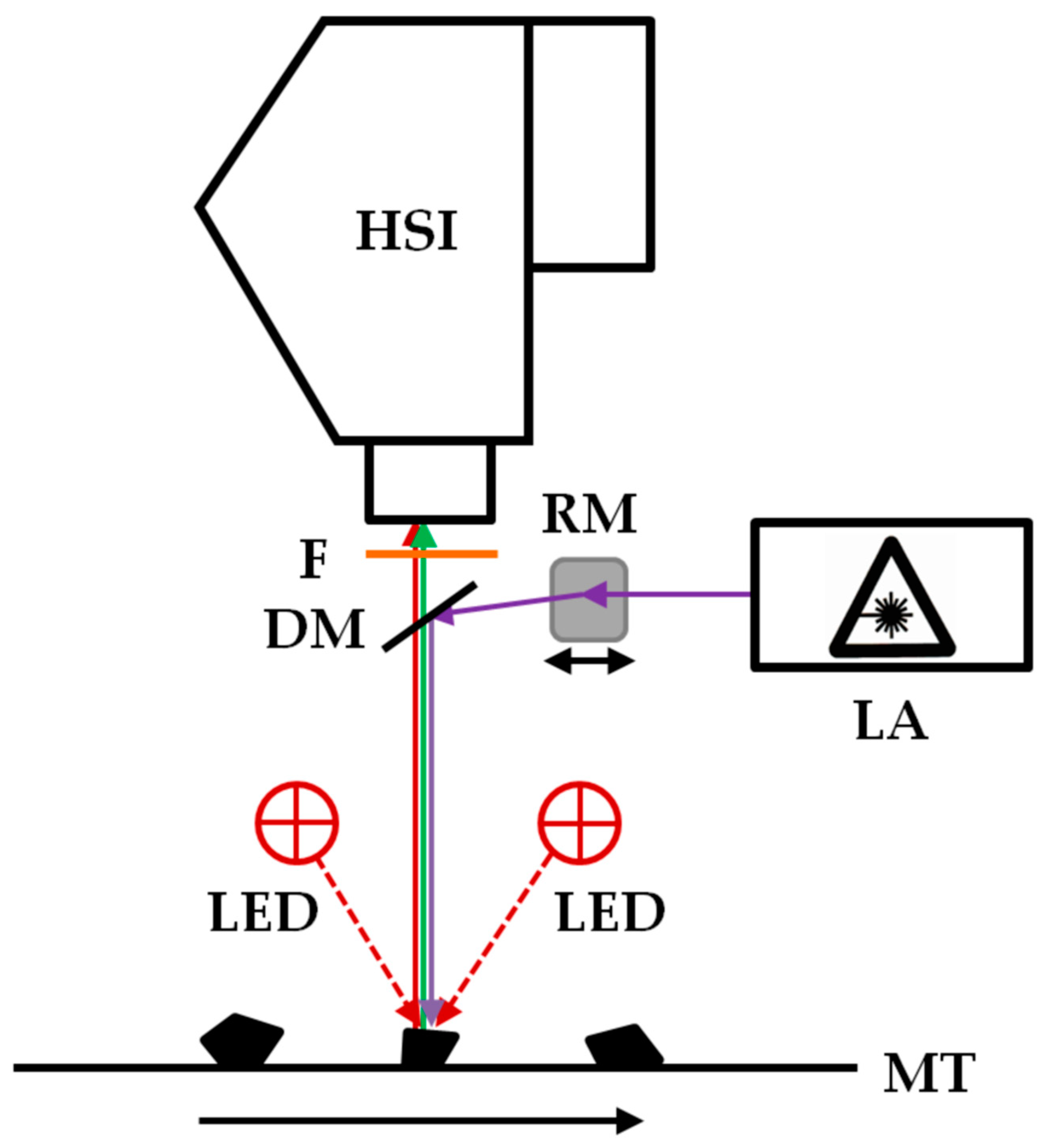
For the investigation of the black polymer particles, an imaging fluorescence spectrometer was used, which was described in detail by Gruber et. al. [26]. A schematic representation of the system is shown in Figure 1. It consists of an excitation laser with a wavelength of 450 nm and an output power of 2000 mW (4290 2W 450 nm Blue Dot Laser Module, Wuhan Besram Technology Inc., Wuhan, China), a rotating mirror (dynAxis S, Scanlab, Puchheim, Germany), a dichroic mirror with an cut-off frequence of 473 nm (Di03-R473, Semrock Inc., Rochester, NY, USA), a long pass filter with an edge wavelength of 458 nm (LP03-458RE, Semrock Inc., Rochester, NY, USA), and a visible and near infrared (wavelength range 400 nm to 1000 nm) hyperspectral camera (Hyperspec-VNIR, Headwall Photonics Inc., Bolton, MA, USA) with a Si-EMCCD detector with 1004 × 1002 pixels (Luca R 604, Andor Technology Ltd., Belfast, UK) and a lens with a focal length of 23 mm and a maximum aperture of f/1.4 (Xenoplan 23 mm f/1.4; Jos. Schneider Optische Werke, Bad Kreuznach, Germany). Lasers with other wavelengths were tested, but the 450 nm lasers provided the best compromise of achievable fluorescence and price performance ratio. In addition to the excitation laser, near-infrared LEDs with a wavelength of 870 nm (Vishay IR diode, RS Components GmbH, Frankfurt am Main, Germany) are used as additional illumination sources. The samples are moved with a linear stage (VT 80, PI Micos, Eschbach, Germany). The control of the system components and the data acquisition is carried out by software developed in-house (Imanto®pro, Fraunhofer IWS, Dresden, Germany).
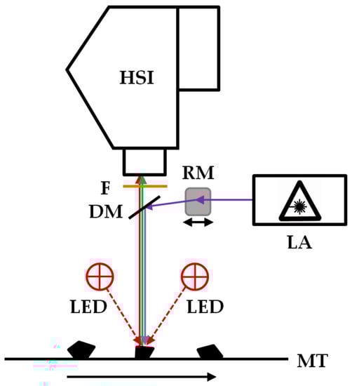
Figure 1.
Schematic representation of the imaging fluorescence spectrometer for the classification of black plastics. HSI: visible and near-infrared HSI camera. DM: Dichroic mirror. LED: near-infrared LEDs λ = 870 nm. F: Long pass filter. GM: Rotating mirror. LA: Excitation laser. MT: motion unit.
2.3. Data Acquisition and Preprocessing
The measurements of the black plastic particles were performed with the described imaging fluorescence spectrometer. The measurements were performed with a working distance of 280 mm, an exposure time of 25 ms, a recording frequency of 22 Hz, a gain of 2×, and 2× binning in the spectral and lateral dimensions. This results in a FOV of ~90 mm, a lateral resolution of ~360 μm, and a spectral resolution of ~1.5 nm. The velocity of the motion unit was set to 4 m s−1 to obtain square pixels. For the measurement, about 40 particles each were separated from each other and placed under the camera. Ten measurements were performed for each polymer, resulting in around 400 particles per plastic. The result of each measurement was one hypercube with a lateral size of ~1000 × 1000 pixel and 380 spectral bands between 400 nm and 1000 nm. The raw data of the measurements can be found in [27].
After data acquisition, the polymer particles in the hypercubes were separated from the substrate by a threshold value based on their NIR reflectivity at 870 nm. Very small particles with a size of less than 10 pixels (<0.5 mm side length) were removed from the data. Subsequently, the wavelength range of the hypercubes of the polymer particles was cut to 103 spectral channels between 501 nm and 664 nm. No fluorescence is to be expected outside these wavelengths.
2.4. Classification Experiments
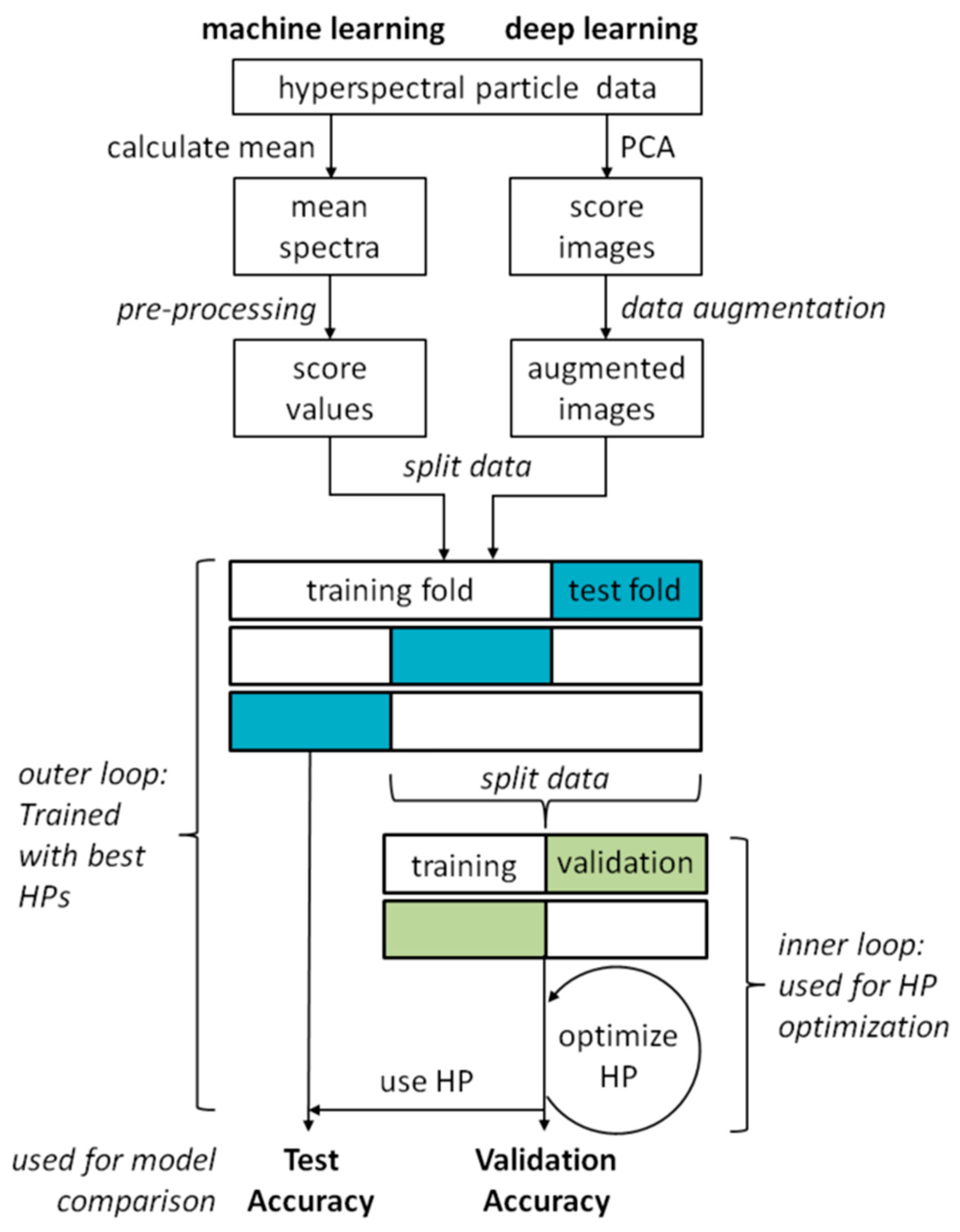
The sequence of the classification experiments including the pre-processing of the data and the optimization of the hyperparameters of the classification models is shown in Figure 2. Algorithms from ‘classical’ machine learning as well as from deep learning were used. In both approaches, the pre-processing of the data differs, while training and validation are the same. The individual steps are described in more detail in the following sections.
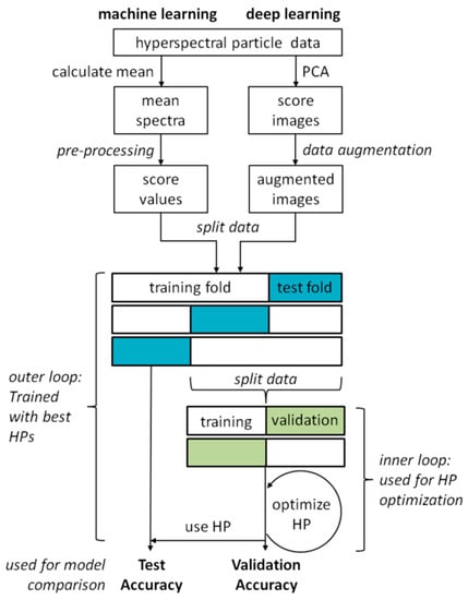
Figure 2.
Schematic representation of the classification experiment procedure with hyperparameter (HP) optimization.
Different data sets were considered for the classification attempts. The overall model of all measured plastic particles was considered (see chapter 2.1). In total, 5534 particles were used for the experiments. The overall model was used to compare the algorithms with regard to their overall classification accuracy and to estimate the influence of automatic hyperparameter optimization. Forty-one industrially relevant plastic mixtures with a maximum of three classes were considered (see Table A3). These data sets are based on actual plastic mixtures, in particular from the automotive and electronics industries. They thus enable a good estimation of the suitability of the imaging fluorescence method for the high-purity sorting of technical black plastic waste.
All calculations were performed with Matlab® R2017b and a Windows 10TM computer with an Intel® CoreTM i5-4590 with 3.3 GHz, 16 GB RAM and a Nvidia® GTX 1080 Ti graphics card with 11 GB GDDR5X memory and a processor clock of 1632 MHz.
2.4.1. Machine Learning
The first approach is to classify the mean spectra of the fluorescence of the plastic particles after pre-processing and principal component analysis [28] using classical machine learning algorithms. Four classification algorithms were compared—linear discriminant analysis (LDA [21]), k-nearest neighbour classification (kNN [22]), classification ensembles with decision trees (ENSEMBLE [24]), and support vector machines (SVM [23]) with a radial basis and linear kernel.
For these experiments, a mean spectrum was calculated for each plastic particle. Subsequently, the spectra were subjected to a data pre-processing consisting of principal component analysis and sometimes Savitzky-Golay smoothing [29] and normalization. Savitzky-Golay smoothing is a frequently used method for smoothing in spectroscopy. The obtained data set can then be used for training the classification models. The classification models were validated by tenfold cross-validation. For this purpose, each data set is divided into 10 parts, and then 10 classification models are trained, whereby one part of the data is always not taken into account for training. The obtained model is then applied to the part of the data not considered, and the overall classification accuracy is determined. The mean value of all 10 tests gives the cross-validated overall accuracy.
2.4.2. Deep Learning
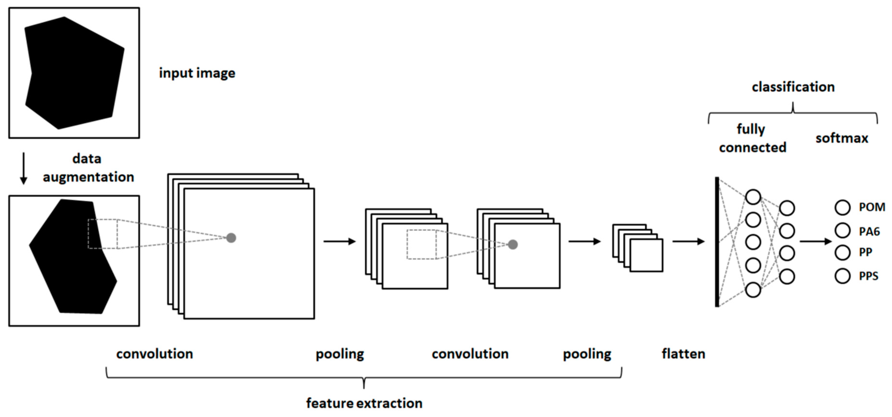
In the second approach, classification experiments were carried out using CNNs [18]. CNNs are a method of deep learning which can achieve very good results in the classification of image data. CNNs consist of artificial neurons arranged in several stacked layers (Figure 3). Typical CNNs consist of one or more convolutional layers followed by pooling layers. After some repetitions of convolutional and pooling layers, they can be followed by fully connected layers. The output of all layers is transformed by an activation function (often reLu function). The output of the fully connected layer is then transformed into a probability function. To avoid an overfitting of the CNNs dropout layer, augmentation of the input images or regularization methods like early stopping can be used. CNNs are trained with backpropagation in a supervised manner [18]. An example configuration of a CNN is show in Figure A1.
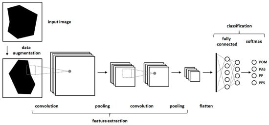
Figure 3.
A schematic structure of a convolutional neural network (CNN).
Before the actual classification experiments, the hypercubes of the HSI measurement had to be converted into an image with less spectral channels. For this purpose, a principal component analysis was first performed with all particle spectra [28]. A new image (called a score image) was then created for each polymer particle using the scores obtained from the first three principal components. The obtained scores were then scaled by nearest-neighbour interpolation to a size of 64 × 64 pixels. The obtained data set from the score images of the plastic particles and the associated classes was then used for the training of the CNNs. The validation of the CNNs is done by fivefold cross-validation. After each epoch of the training, the overall accuracy for the validation set was calculated. The training of the CNNs was aborted if, after five consecutive training epochs, no improvement of the overall classification accuracy for the validation data set could be determined. This method is called early stopping and is used to reduce overfitting during training.
Since the training of CNNs is very computationally intensive, it is not always useful to train a new CNN from scratch. Especially with similar classification problems, it is possible to use an already trained CNN as a starting point for a model for a new classification problem. This method is called transfer learning [30]. Transfer learning is used here for the classification attempts of the 41 industrial relevant plastic mixtures. Therefore, the best received CNN trained for the classification of all plastics is used. The learned weights of the neurons of this CNN are used as a starting point for the training of a new CNN for the new classification problem. For this, only the last layers of the original CNN (the last fully connected and the softmax layer) have to be adapted to the new classification problem, and then the training can be carried out normally.
2.4.3. Hyperparameter Optimization
Hyperparameters are the parameters of the classification algorithms used to control the algorithms themselves. These parameters are set before the actual training of the models and are not learned during the training. Other parameters, such as the pre-processing of spectral data by smoothing or normalization, can also be considered as hyperparameters. The hyperparameters can have a large effect on the overall classification accuracy of the trained algorithms, which is why an optimization is useful. Often this optimization is guided by trial and error and the experience of the user. This process is often time-consuming and finding an optimal result is not guaranteed. For this reason, methods for automatic hyperparameter optimization are increasingly being used, especially for classification algorithms with high computational effort and many hyperparameters (e.g., CNNs). These algorithms attempt an iterative approach to the optimal hyperparameters of the classification algorithm using various mathematical methods. An example of such an algorithm is the Bayesian Optimization Algorithm (BOA, [31]). A disadvantage of these algorithms is that their calculation itself is time consuming and computationally intensive. A quick and easy alternative is the Random Search algorithm (RS), which selects the next hyperparameter randomly. It has been shown that the differences between RS and other hyperparameter optimization algorithms are often small [25]. Therefore, the RS algorithm is used here for hyperparameter optimization. For this the algorithm implemented in Matlab R2017b was used slightly modified.
Hyperparameter optimization was used both for the ‘classical’ machine learning algorithms and for CNN training. The standard hyperparameters and the ranges in which these parameters were optimized are summarized in Table A1 for classical machine learning and in Table A2 for CNNs. For all algorithms, models with standard hyperparameters (derived from the Matlab® R2017b documentation) were also trained to estimate the effect of automatic hyperparameter optimization.
Hyperparameter optimization using RS was performed on 30 epochs, which means that 30 models with different random hyperparameters were trained to find a good set of hyperparameters. The validation was done by external and internal cross validation. For this purpose, the entire data set is divided into ten (for the classical machine learning algorithms) or five (for the CNNs) parts for the cross validation, and hyperparameter optimization is performed over 30 epochs with each of the partitions. For each part of the data, 30 models with different hyperparameters are trained to achieve good overall classification accuracy. Each of these individual models is in turn validated by five-fold cross-validation (for the classical machine learning algorithms) or two-fold cross-validation (for the CNNs). This is called the inner loop, which is used to optimize the hyperparameters. The model with the best overall classification accuracy found in the inner loop is then used to predict the left out data of the first cross-validation to obtain a good estimate of the real overall accuracy of the model. This is called the outer loop. This approach is shown schematically in Figure 2.
2.4.4. Model Comparison
The classification models are compared using the calculated overall classification accuracies of the cross validation. In order to determine whether there are statistically significant differences between the overall accuracies obtained, the overall accuracies were compared by means of univariate ANOVA and a subsequent Tukey test. The significance level chosen was α = 5%. The prerequisites for the application of ANOVA are the normal distribution and the homoscedasticity of the data. These conditions are checked here by the Anderson-Darling Test [32] and the Brown-Forsythe Test [33]. No deviations from these prerequisites were found for any of the experiments. The third prerequisite of ANOVA is the independence of the examined data. This is only partially given for cross-validation. Although the test data are independent of each other, since each data point appears only once in a test data set, the training data are not independent, since one data point is used several times for training. It has been shown that this dependency leads to a slightly increased Type 1 error when comparing different data sets [34]. This would mean that the ANOVA indicates a statistically significant difference, although none exists between the overall accuracies of the classification models. However, we accept the increased error here because the expected increase is small and because we do not have enough data to run the experiments with independent training, validation, and test sets. In addition, the effect of a slightly increased error probability is also small, and the method is nevertheless sufficient for comparing different classification methods.
3. Results and Discussion
3.1. Imaging Fluorescence Measurements
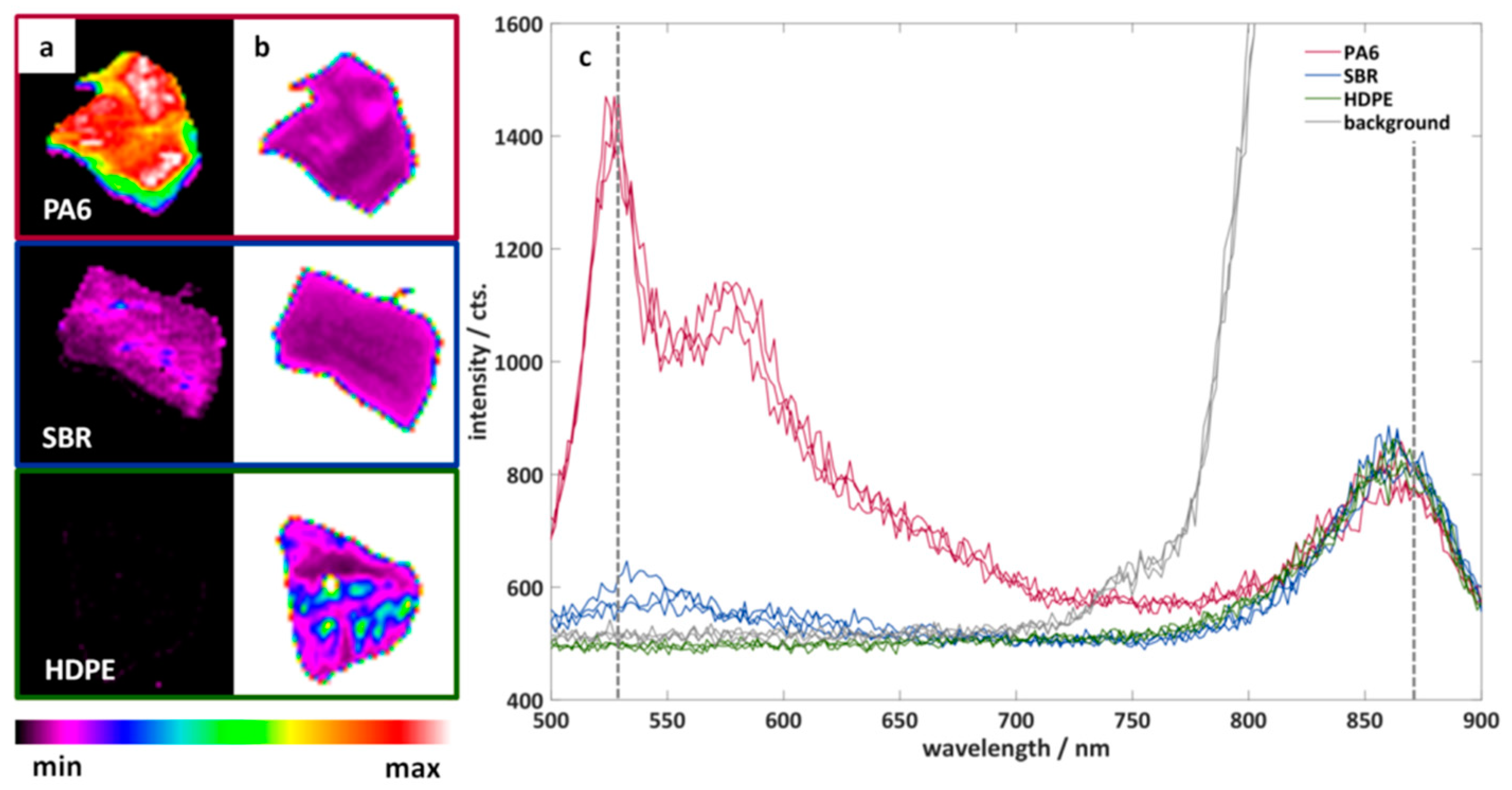
Figure 4 shows example measurements of three particles of different black plastics. The three plastics have different fluorescence properties: PA6 shows a clear fluorescence, SBR shows only a partial fluorescence, and HDPE shows no fluorescence. The additional illumination (870 nm) and measurement of the samples in the NIR spectral range is of particular importance for the measurement of HDPE. This makes it possible to measure the position and shape of non-fluorescent plastics. In addition, a simple differentiation between the background and the particles is easily possible.
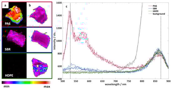
Figure 4.
Color-coded fluorescence intensity of three particles of black plastics measured with the imaging fluorescence spectrometer at a wavelength of (a) 530 nm and (b) 870 nm. (c) Example spectra of the three plastic particles. Red: polyamide 6 (PA6). Blue: styrene-butadiene rubber (SBR). Green: high-density polyethylene (HDPE). Grey: background.
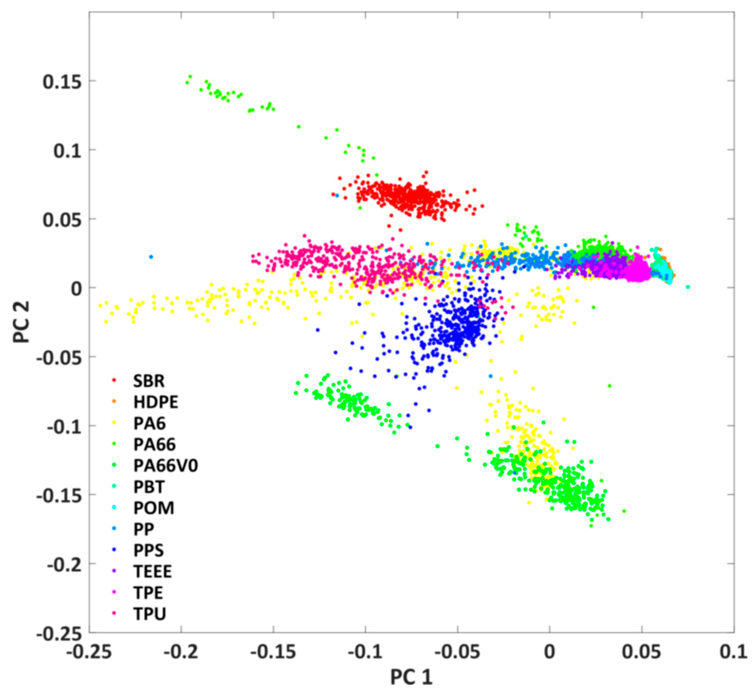
It can be seen that the shape of the plastic particles is well represented and that there are clear spectral differences between PA6 and SBR. In a next step, the fluorescence of all investigated plastics should be compared in order to estimate the spectral differentiability of the plastics. For this purpose, the hypercubes obtained were pre-processed as described in Chapter 2.3. The results are the mean value spectra of all measured plastic particles. A principal component analysis was applied to this data set after L1 normalization. Figure 5 shows the score plot of the first and second principal components. The first two principal components describe 95% of the variance of the data set. Each point in the score plot corresponds to the mean spectrum of a plastic particle. Similar spectra are close together in the score plot, while different spectra are separated.
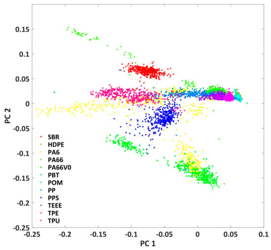
Figure 5.
Score plot of the first and second principal component of the principal component analysis of the mean value spectra of all studied plastic particles.
It can be seen that some of the plastics (e.g., SBR and PPS) are spectrally different from the others. However, some of the investigated samples also show clear overlaps (e.g., TPE, TPU, and TEEE) in the score plot. For these plastics, classification on the basis of spectral properties is probably more difficult. For these plastics, the classification can possibly be improved by considering the particle shape. Furthermore, it can be seen that the plastics PA6 and PA66 exhibit a large spectral variability and can be found at several positions in the score plot. This might be due to the fact that plastics with and without glass fibre additives are regarded as one plastic class. Overall, however, the score plot only provides an initial indication of the possibility of classifying plastics.
3.2. Classification Experiments
3.2.1. Classification of all Plastics by a Single Prediction Model
First, the classification experiments were carried out with a data set from all 12 plastic classes as a worst-case scenario. In the real recycling process, it is usually not necessary to identify and sort more than two or three different plastics. The calculation of the classification models serves to compare the performance of the different algorithms for the classification of the black plastic particles and to estimate the practicability of the automatic hyperparameter optimization. Only the evaluation for the overall accuracy and not for other accuracy measures, like kappa coefficients, is shown.
The models were trained once with the standard hyperparameters for the classification algorithms taken from the Matlab® R2017b documentation. In addition, the hyperparameters of the models were optimized using RS. No pre-processing or data augmentation takes place during these tests. For optimization using RS, the value range of the hyperparameters was also determined on the basis of the Matlab® R2017b documentation. The standard hyperparameters and their ranges for the optimization are shown in Table A1 for the algorithms LDA, kNN, SVM, and ENSEMBLE and in Table A2 for the CNNs. A total of seven hyperparameters must be optimized for the DA algorithm, eight for the kNN algorithm, eight for the SVM, 10 for the ENSEMBLE algorithm, and 17 for the CNN.
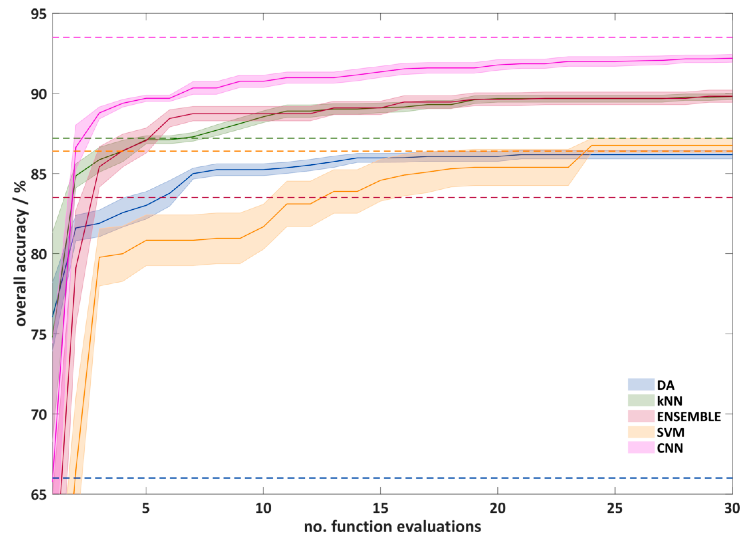
Figure 6 shows the course of the automatic hyperparameter optimization using RS. The plot shows the test accuracy (overall accuracy, often the outer loop) against the number of function evaluations performed. It can be seen that, after 10 calculated functions, significantly better hyperparameters were found. Between 10 and 25 function evaluations, only a slight improvement can be seen. After 25 function evaluations, only the CNNs show a slight improvement. The reason for this is probably the larger number of possible hyperparameter combinations for the CNNs. However, since the improvements after 30 function evaluations are also small for the CNNs and the computational effort is high, a termination of the experiments after 30 function evaluations seems reasonable. It can also be seen that the optimization for the SVMs works worst, which results in a slow increase of the average overall classification accuracy and a large standard deviation. After the optimization the overall classification accuracy (86.8%) is comparable with that of the DA algorithm (86.2%). For the remaining algorithms, the CNNs show the best results (92.2%). kNN and ENSEMBLE algorithms lead to very similar results (89.8%), and the DA provides a much lower overall classification accuracy.
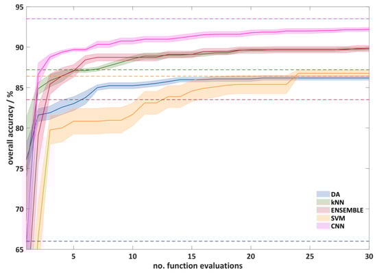
Figure 6.
The overall cross-validation accuracy of the outer loop as a function of the number of function evaluation in automatic hyperparameter optimization using random search (RS) optimization. For a better overview, only a quarter of the standard deviation is shown. The dashed lines show the overall classification accuracy with the standard hyperparameter.
Table 1 shows the comparison of the obtained overall classification accuracies and the kappa coefficients of the RS-optimized models and the overall accuracies and kappa coefficients of the models trained with standard hyperparameters. Only the overall accuracy is discussed here, because the results for the kappa coefficients are very similar. The highest overall accuracy is achieved for the CNNs, where the overall accuracy for the models trained with standard parameters is higher than for the models optimized with RS. However, the difference is small at 1.5%. With the other algorithms, higher overall classification accuracies are achieved using RS. The differences in the overall accuracies are statistically relevant for all algorithms except the SVMs, with a significance level of α = 5%. This result shows that the automatic optimization of the hyperparameters is suitable for the training of good classification models. With the CNN models, the high number of hyperparameters to be optimized probably leads to the worse result of the optimization. Perhaps training more models would further improve overall classification accuracy. However, this also results in a longer training time, which is already very long, especially for the CNNs.

Table 1.
Comparison of the obtained average overall classification accuracies and kappa coefficients with confidence intervals (α = 0.05) of the experiments with all 12 black plastics, with and without hyperparameter optimization. The best overall classification accuracy is shown in bold. The asterix (*) shows a statistically significant difference between the models trained with standard parameters and the models trained with RS (calculated with ANOVA, α = 0.05).
Overall, it can be seen that the best classification accuracy of 93.5% can be achieved with the CNNs for the classification of all 12 plastic classes. This result is statistically significantly better than the overall classification accuracy of the other models. In the classical machine learning algorithms, kNN and ENSEMBLE deliver the same overall classification accuracy of 89.8% and are thus statistically significantly better than the SVM and DA models. For these models, 86.8% and 86.2% overall classification accuracy, respectively, are achieved. For a further application, it makes more sense to use the ENSEMBLE instead of the kNN algorithm, since kNN models often require a lot of memory space and only allow a low prediction speed [21].
3.2.2. Classification of Relevant Plastic Mixtures by Individual Prediction Models
After the classification experiments with all investigated plastic particles, further experiments for the classification of 41 mixtures of a maximum of three different plastic classes were carried out. A total of 41 plastic mixtures were selected which correspond to them typically expected to receive at a recycling company (see Table A3). The number of samples per plastic class is shown in Section 2.1.
The following six models were trained for all mixtures:
For transfer learning, the best CNN for the classification of all plastic particles from Section 3.2.1 was selected. The training and the validation were carried out as for the models for the classification of all plastic classes.
The results of the experiments are presented in Table 2. The results for the kappa coefficients are not shown because the results are very similar. It can be seen that both the models with hyperparameter optimization by random search for the ENSEMBLE and SVM models and the CNNs trained with transfer learning are better than the models trained with the standard parameters. For ENSEMBLE and SVM, the mean improvement in overall classification accuracy is 0.7 percentage points and 1.9 percentage points, respectively. For the CNNs, the difference is even 21.7 percentage points. This large difference indicates that the completely new training of the CNNs does not work well for the data sets studied. One possible reason for this is the relatively low number of training images available for CNN training. When using transfer learning, the CNN only has to be adapted to the new data set, for which a smaller data set is sufficient. The results show that both automatic hyperparameter optimization and transfer learning are good methods for increasing the overall accuracy of the algorithms used. This would enable the relatively fast training of new algorithms even for untrained personnel in a later industrial application.
Table 2.
Results of the classification attempts of the 41 individual models considered. The highest overall classification accuracy is shown in bold. For reasons of clarity, the confidence interval of the tests is not shown. Only the overall accuracy is shown because the results for the kappa coefficient are very similar.
A possible disadvantage could be the relatively long training times, especially for the use of hyperparameter optimization by random search. For the data sets considered here, however, the average training time per model is only 220 s for the ENSEMBLE algorithm and 273 s for the SVM algorithm (Table 3). For transfer learning, the average training time is only 54 s. However, when increasing the number of training data, which may be necessary to improve the overall classification accuracy, the training times may increase considerably.
Table 3.
Average training times for the classification algorithms used. The ensemble learning with decision trees (ENSEMBLE) and support vector machine (SVM) models were trained with RS for 30 function evaluations with 10-fold cross-validation in the outer loop and five-fold cross-validation in the outer loop. The CNN models were trained with transfer learning and validated with five-fold cross-validation.
The average overall accuracy of all three algorithms is 99.0%. In total, 18 of the 41 plastic combinations achieved an overall classification accuracy of 99.9% or better, and 25 had an overall classification accuracy of more than 99.5%. The consideration of the particle shape through the use of CNNs did not on average lead to an improvement of the overall classification accuracy in the experiments with the plastic mixtures. A possible reason for this can also be found in the relatively small number of training examples. Since CNNs especially benefit from large amounts of training data, it might be possible to improve the overall classification accuracy by further data.
Further experiments should therefore concentrate on the generation of more data for the training of the classification algorithms. Furthermore, the development of a technical demonstrator is planned. The aim is to further investigate the suitability of imaging fluorescence spectroscopy technology for the classification of black plastics. Further development of the sensor system, in particular the excitation unit and the system for generating the laser line, is also planned. In addition, other HSI cameras will be investigated, which enable faster data acquisition and thus lead to a higher plastic throughput in later use.
4. Conclusions
In this study, an imaging fluorescence spectrometer with additional illumination in the NIR spectral range was used to classify technical black plastic particles after cryogenic grinding. These plastics are arising in particular during the recycling of plastic components from the automotive or electronics industries. Since these are often composite components, the waste is ground to small particles before recycling and must then be sorted with high purity (99.9%). Even the smallest impurities can reduce the quality of the recycled material and thus the achievable price. A sorting of technical black plastic particles is not yet possible with this purity. The aim was therefore to measure the fluorescence of the black plastics after excitation with a 450 nm laser and to classify them with high overall accuracy using machine learning models. In addition, attempts have been made to use the shape of the plastic particles for classification by using CNNs, thereby increasing the achievable overall classification accuracy.
A total of around 400 particles were measured from 14 plastics in 12 plastic classes. The classification was carried out using the algorithms discriminant analysis, k nearest neighbour classification, support vector machines, classification ensembles with decision trees, and convolutional neural networks. It was also attempted to find optimal model parameters, which can significantly increase the overall classification accuracy of the models. These parameters were determined by an automatic hyper parameter optimization by random search.
The experiments with the total data set of all plastics showed that the best results could be achieved using CNNs, kNN, and ENSEMBLE algorithms. The highest overall classification accuracy was 93.5% for the CNNs. Hyperparameter optimization led to a statistically significant improvement in overall classification accuracy for most algorithms.
When considering 41 plastic mixtures with two to three plastic per mixture, the desired overall accuracy of at least 99.9% was achieved for 18 of the plastic mixtures. Here, the use of CNNs showed no improvement compared to ENSEMBLE and SVM algorithms. In the future, an industry-oriented demonstrator for the classification of technical black plastic particles using imaging fluorescence spectroscopy will be developed, and more data is to be recorded for the training of better models.
Overall, the method presented seems to be a promising approach for the classification of black plastics and could contribute to an increase in the recycling of plastic waste.
Author Contributions
F.G. conducted the research presented in this study and wrote the paper. W.G., P.W., and S.K. contributed to the development of the overall research design, provided guidance along the way, and aided in writing of the paper.
Funding
This research was funded by the scholarship program of the Deutsche Bundesstiftung Umwelt grant number 20016/421 and by the Sächsische Aufbaubank of the state of Saxony.
Acknowledgments
Special thanks go to Beate Leupold, Oliver Throl, and Susann Kleber. Thanks to Kunststoffrecycling CKT GmbH & Co KG for providing the black plastic samples.
Conflicts of Interest
The authors declare no conflict of interest.
Appendix A
Table A1.
Overview of the default values and the optimization ranges of the hyperparameters of the classical machine learning models. For a description of the hyperparameters, please refer to the literature references.
Table A1.
Overview of the default values and the optimization ranges of the hyperparameters of the classical machine learning models. For a description of the hyperparameters, please refer to the literature references.
| Hyperparameter | Standard Value | Optimization Range | |
|---|---|---|---|
| for all algorithms | Savitzky-Golay smoothing | no | yes/no |
| polynomial degree for Savitzky-Golay smoothing | - | 1–5 | |
| data points for Savitzky-Golay smoothing | - | 3–21 | |
| normalization | none | none/L1/L2/Linf/SNV/min-max | |
| No. of PCs used | 10 | 2–20 | |
| discriminant analysis (DA) [35] | delta | 0 | 0–1 |
| gamma | 0 | 0–1 | |
| k-nearest neighbours (kNN) [36] | number of neighbors | 3 | 1–11 |
| distance metric | euclidean | euclidean/cityblock/cosine | |
| distance weight | equal | equal/invers/quadratic-invers | |
| ensemble learning with decision trees (ENSEMBLE) [37] | ensemble method | AdaBoost | Bag / RusBoost / AdaBoost |
| No. of decision trees | 100 | 10–500 | |
| learnrate | 1 | 0.001–1 | |
| max. number of decision splits | 1 | 1–100 | |
| min. leaf size | 1 | 1–100 | |
| support vector machines (SVM) [38] | kernel | rbf | rbf/linear |
| box-constraint | 1 | 0.001–1000 | |
| kernel-scale | 1 | 0.001–1000 |
Table A2.
Overview of the optimization ranges of the hyperparameters of the CNN models. For a description of the hyperparameters, please refer to the literature references.
Table A2.
Overview of the optimization ranges of the hyperparameters of the CNN models. For a description of the hyperparameters, please refer to the literature references.
| Hyperparameter | Standard Value | Optimization Range | |
|---|---|---|---|
| data augmentation [39] | reflexion | no | yes/no |
| rotation | 0 | 0–360° | |
| translation | 0 | 0–16 pixel | |
| scaling | 1 | 1–1.25 | |
| shearing | 0 | 0–25% | |
| network topologie [40] | No. of convolution blocks | 4 | 2–4 |
| convolution layer per block | 1 | 1–3 | |
| No. of filters of the 1st convolution layer 1 | 16 | 8–48 | |
| size of the convolution kernel | 3 × 3 | 1 × 1; 3 × 3; 5 × 5; 7 × 7 | |
| pooling mode | max-pooling | average-pooling; max-pooling | |
| No. of fully connected layer | 1 | 1–3 | |
| No. of neurons per fully connected layer | 50 | 25; 50; 75; 100; 150; 200 | |
| dropout possibility after last pooling layer 2 | 0 | 0–50% | |
| training parameter [41] | momentum | 0.95 | 0.5–0.999 |
| learnrate | 0.01 | 0.001–1 | |
| L2 regularisation | 0.0005 | 0.0001–1 |
1 The number of filters doubles after each convolution block. 2 There was no dropout at different places of the CNN.
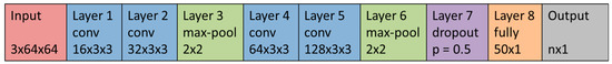
Figure A1.
Schematic representation of a sample CNN. The CNN has two convolution blocks with two convolution layers per block. The kernel size of the convolution layer is 3 × 3. The CNN uses max-pooling with a pooling size of 2 × 2. After the last pooling layer is a dropout layer with a dropout probability of 50%. There is one fully connected layer with 50 neurons. The reLu-Layers are not shown in this image.
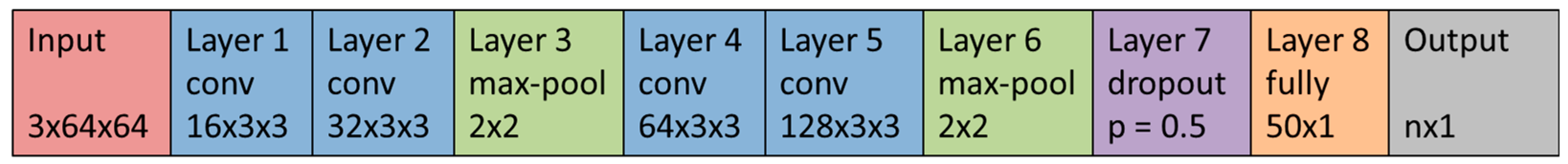
Table A3.
Overview of the plastic mixtures considered for the classification tests.
Table A3.
Overview of the plastic mixtures considered for the classification tests.
| Abbreviation | Polymers | Abbreviation | Polymers |
|---|---|---|---|
| M1 | HDPE|PP | M22 | PBT|TEEE |
| M2 | PA6|Gummi | M23 | PA6|TPE-HDPE |
| M3 | PA6|PBT | M24 | PA6|TPE-PBT |
| M4 | PA6|POM | M25 | PA6|TPE-PP |
| M5 | PA6|PPS | M26 | PA6|TPU-POM |
| M6 | PA6|TPE | M27 | PA6|TPU-TPE-TEEE |
| M7 | PA6|TPU | M28 | PA66|TPE-HDPE |
| M8 | PA6|PA66 | M29 | PA66|TPE-PBT |
| M9 | PA6|TEEE | M30 | PA66|TPE-PP |
| M10 | PA66|Gummi | M31 | PA66|TPU-POM |
| M11 | PA66|PBT | M32 | PA66|TPU-TPE-TEEE |
| M12 | PA66|POM | M33 | PBT|TPU-TPE-TEEE |
| M13 | PA66|PPS | M34 | PA6|TPE|HDPE |
| M14 | PA66|TPE | M35 | PA6|TPE|PBT |
| M15 | PA66|TPU | M36 | PA6|TPE|PP |
| M16 | PA66|PA66V0 | M37 | PA6|TPU|POM |
| M17 | PA66|TEEE | M38 | PA66|TPE|HDPE |
| M18 | PBT|Gummi | M39 | PA66|TPE|PBT |
| M19 | PBT|PP | M40 | PA66|TPE|PP |
| M20 | PBT|TPE | M41 | PA66|TPU|POM |
| M21 | PBT|TPU |
References
- Geyer, R.; Jambeck, J.R.; Law, K.L. Production, use, and fate of all plastics ever made. Sci. Adv. 2017, 3, e1700782. [Google Scholar] [CrossRef] [PubMed]
- Wang, C.-Q.; Wang, H.; Fu, J.-G.; Liu, Y.-N. Flotation separation of waste plastics for recycling—A review. Waste Manag. 2015, 41, 28–38. [Google Scholar] [CrossRef] [PubMed]
- Hearn, G.L.; Ballard, J.R. The use of electrostatic techniques for the identification and sorting of waste packaging materials. Resour. Conserv. Recycl. 2005, 44, 91–98. [Google Scholar] [CrossRef]
- Kulcke, A.; Gurschler, C.; Spöck, G.; Leitner, R.; Kraft, M. On-line classification of synthetic polymers using near infrared spectral imaging. J. Near Infrared Spectrosc. 2003, 11, 71–81. [Google Scholar] [CrossRef]
- Serranti, S.; Gargiulo, A.; Bonifazi, G. Hyperspectral imaging for process and quality control in recycling plants of polyolefin flakes. J. Near Infrared Spectrosc. 2012, 20, 573–581. [Google Scholar] [CrossRef]
- Riise, B.L.; Biddle, M.B.; Fisher, M.M. X-Ray Fluorescence Spectroscopy in Plastic Recycling; American Plastics Council: Arlington, VA, USA, 2000. [Google Scholar]
- Rozenstein, O.; Puckrin, E.; Adamowski, J. Development of a new approach based on midwave infrared spectroscopy for post-consumer black plastic waste sorting in the recycling industry. Waste Manag. 2017, 68, 38–44. [Google Scholar] [CrossRef] [PubMed]
- EVK DI KERSCHHAGGL GMBH. Black Polymer Sorting. Available online: http://www.bp-sorting.com/uploads/4/7/5/6/4756078/bp_sorting_-_laymans_report.pdf (accessed on 14 September 2015).
- Küter, A.; Reible, S.; Geibig, T.; Nüßler, D.; Pohl, N. THz imaging for recycling of black plastics. Tech. Mess. 2018, 85, 191–201. [Google Scholar] [CrossRef]
- Mikloweit, M. Sortierung Schwarzer Kunststoffe für Recycling. Available online: http://www.blackvalue.de/ (accessed on 25 June 2019).
- Shameem, K.M.M.; Choudhari, K.S.; Bankapur, A.; Kulkarni, S.D.; Unnikrishnan, V.K.; George, S.D.; Kartha, V.B.; Santhosh, C. A hybrid LIBS-Raman system combined with chemometrics: An efficient tool for plastic identification and sorting. Anal. Bioanal. Chem. 2017, 409, 3299–3308. [Google Scholar] [CrossRef]
- Unnikrishnan, V.K.; Choudhari, K.S.; Kulkarni, S.D.; Nayak, R.; Kartha, V.B.; Santhosh, C. Analytical predictive capabilities of Laser Induced Breakdown Spectroscopy (LIBS) with Principal Component Analysis (PCA) for plastic classification. RSC Adv. 2013, 3, 25872. [Google Scholar] [CrossRef]
- Heckmann, W. Characterization of polymer materials by fluorescence imaging. Microsc. Microanal. 2005, 11, 2036–2037. [Google Scholar] [CrossRef]
- Hawkins, K.R.; Yager, P. Nonlinear decrease of background fluorescence in polymer thin-films—A survey of materials and how they can complicate fluorescence detection in μTAS. Lab Chip 2003, 3, 248–252. [Google Scholar] [CrossRef] [PubMed]
- Soutar, I. The application of luminescence techniques in polymer science. Polym. Int. 1991, 26, 35–49. [Google Scholar] [CrossRef]
- UniSensor Sensorsysteme GmbH. POWERSORT 200. Available online: http://www.unisensor.de/en/products/product-details/recycling-industry-1/powersort-200-1.html (accessed on 1 July 2019).
- Suryanarayana, C. Mechanical alloying and milling. Prog. Mater. Sci. 2001, 46, 1–184. [Google Scholar] [CrossRef]
- Goodfellow, I.; Bengio, Y.; Courville, A. Deep Learning, Adaptive Computation and Machine Learning Series; MIT Press: Cambridge, MA, USA, 2016. [Google Scholar]
- Krizhevsky, A.; Sutskever, I.; Hinton, G.E. ImageNet classification with deep convolutional neural networks. In Advances in Neural Information Processing Systems 25; Pereira, F., Burges, C.J.C., Bottou, L., Weinberger, K.Q., Eds.; Curran Associates, Inc.: Red Hook, NY, USA, 2012; pp. 1097–1105. [Google Scholar]
- Simonyan, K.; Zisserman, A. Very deep convolutional networks for large-scale image recognition. arXiv 2014, arXiv:1409.1556. [Google Scholar]
- Bishop, C.M. Pattern recognition and machine learning, 11. (corr. printing). In Information Science and Statistics; Springer: New York, NY, USA, 2013. [Google Scholar]
- Cover, T.; Hart, P. Nearest neighbor pattern classification. IEEE Trans. Inform. Theory 1967, 13, 21–27. [Google Scholar] [CrossRef]
- Steinwart, I.; Christmann, A. Support vector machines. In Information Science and Statistics; Springer: New York, NY, USA, 2008. [Google Scholar]
- Breiman, L.; Friedman, J.H.; Olshen, R.A.; Stone, C.J. Classification and Regression Trees; Chapman & Hall/CRC: Boca Raton, FL, USA, 2017. [Google Scholar]
- Bergstra, J.; Bengio, Y. Random search for hyper-parameter optimization. J. Mach. Learn. Res. 2012, 13, 281–305. [Google Scholar]
- Gruber, F.; Wollmann, P.; Grählert, W.; Kaskel, S. Hyperspectral imaging using laser excitation for fast raman and fluorescence hyperspectral imaging for sorting and quality control applications. J. Imaging 2018, 4, 110. [Google Scholar] [CrossRef]
- Gruber, F. Imaging Fluorescence Measurements of Black Plastic Particles Measured with 450 nm Excitation. figshare. Dataset. Available online: https://doi.org/10.6084/m9.figshare.9205292 (accessed on 11 September 2019).
- Jolliffe, I. Principal Component Analysis; Springer: New York, NY, USA, 2011. [Google Scholar]
- Savitzky, A.; Golay, M.J.E. Smoothing and differentiation of data by simplified least squares procedures. Anal. Chem. 1964, 36, 1627–1639. [Google Scholar] [CrossRef]
- Yosinski, J.; Clune, J.; Bengio, Y.; Lipson, H. How transferable are features in deep neural networks? In Advances in Neural Information Processing Systems 27; Ghahramani, Z., Welling, M., Cortes, C., Lawrence, N.D., Weinberger, K.Q., Eds.; Curran Associates, Inc.: Red Hook, NY, USA, 2014; pp. 3320–3328. [Google Scholar]
- Snoek, J.; Larochelle, H.; Adams, R.P. Practical bayesian optimization of machine learning algorithms. In Advances in Neural Information Processing Systems 25; Pereira, F., Burges, C.J.C., Bottou, L., Weinberger, K.Q., Eds.; Curran Associates, Inc.: Red Hook, NY, USA, 2012; pp. 2951–2959. [Google Scholar]
- Anderson, T.W.; Darling, D.A. Asymptotic theory of certain “goodness of fit” criteria based on stochastic processes. Ann. Math. Stat. 1952, 23, 193–212. [Google Scholar] [CrossRef]
- Brown, M.B.; Forsythe, A.B. Robust tests for the equality of variances. J. Am. Stat. Assoc. 1974, 69, 364–367. [Google Scholar] [CrossRef]
- Dietterich, T.G. Approximate statistical tests for comparing supervised classification learning algorithms. Neural Comput. 1998, 10, 1895–1923. [Google Scholar] [CrossRef] [PubMed]
- The MathWorks, Inc. Fitcdiscr: Fit Discriminant Analysis Classifier. Available online: http://de.mathworks.com/help/stats/fitcdiscr.html (accessed on 5 July 2019).
- The MathWorks, Inc. Ficknn: Fit K-Nearest Neighbor Classifier. Available online: http://de.mathworks.com/help/stats/fitcknn.html?s_tid=doc_ta (accessed on 5 July 2019).
- The MathWorks, Inc. Fitcensemble: Fit Ensemble of Learners for Classification. Available online: http://de.mathworks.com/help/stats/fitcensemble.html?s_tid=doc_ta (accessed on 5 July 2019).
- The MathWorks, Inc. Fitcecoc: Fit Multiclass Models for Support Vector Machines or Other Classifier. Available online: http://de.mathworks.com/help/stats/fitcecoc.html?s_tid=doc_ta (accessed on 5 July 2019).
- The MathWorks, Inc. imageDataAugmenter: Configure Image Data Augmentation. Available online: http://de.mathworks.com/help/deeplearning/ref/imagedataaugmenter.html?s_tid=doc_ta (accessed on 5 July 2019).
- The MathWorks, Inc. List of Deep Learning Layers. Available online: http://de.mathworks.com/help/deeplearning/ug/list-of-deep-learning-layers.html (accessed on 5 July 2019).
- The MathWorks, Inc. TrainNetwork: Train Neural Network for Deep Learning. Available online: http://de.mathworks.com/help/deeplearning/ref/trainnetwork.html (accessed on 5 July 2019).
© 2019 by the authors. Licensee MDPI, Basel, Switzerland. This article is an open access article distributed under the terms and conditions of the Creative Commons Attribution (CC BY) license (http://creativecommons.org/licenses/by/4.0/).