Abstract
The digitalization of mechanical waste treatment can have a supporting effect in recovering valuable raw materials from mixed solid waste, achieving the EU’s recycling targets, and developing the waste industry into a circular economy. Therefore, influencing factors on machines and the entire plant must be known. Furthermore, optimization potentials can be developed with the help of digital approaches, such as dynamic control of machine and plant operation, to be able to control the heterogeneous material streams to enable optimized treatment and preserve valuable materials. To establish dynamic control in waste treatment machines, sensors are required to record the necessary variable parameters. In this work, the focus of those variables is placed on the volume flow leaving the shredding machine, where a volume flow sensor is used as a sensor system. To predict the volume flow of the shredder’s output to create a possible dynamic control, forecasting with ARIMA models is used. Initial results show that it is possible to predict a heterogeneous material stream with a selected model, currently over a time period of 10 s. However, the testing of additional prediction models still offers the opportunity of predicting the material stream over a longer period of time to enable dynamic control.
1. Introduction
To achieve the target values set by the EU, member states are required to optimize their national waste management towards a circular economy [1,2,3]. Innovative and digital technologies should be used to implement measures to combat climate change. The waste sector must become more sustainable, reliable and transparent through digitalization [4]. Digitalization supports the development towards a circular economy [2,5,6]. In many other industries, digitization and automated work processes are state of the art, in waste treatment, digitalization is also becoming increasingly important, with more and more companies seeing opportunities through digitalization and actively engaging with it [3,7]. In the future, mechanical waste treatment plants are to be controlled dynamically, made possible by the use of different sensors, which provide information about the operating status of the plant, but also information about the qualities, masses, and volumes of the individual material streams after each treatment step. The system should adjust itself automatically according to the quality requirements based on real-time information. Machines should therefore communicate with each other and be coordinated with each other to form an optimized overall system. Environmental legislation will force the waste management industry, among others, to constantly optimize and adapt, but also to innovate further [8]. The digitalization of municipal waste management is inevitable, which was recently also anchored in national legislation, for example, as a crucial method in the Austrian circular economy strategy [2]. On the one hand, the use of technologies could lead to improved efficiency and cost reduction as part of the circular economy, by providing alternative materials (for example, materials from mixed waste). Furthermore, the use of digital technologies can promote sustainability if economic development goes hand in hand with climate and environmental protection [9,10]. Some digital technologies are already in use in the waste treatment sector, such as intelligent containers, artificial intelligence for material characterization, robot automation, and semi-autonomous trucks, which were extensively reviewed by the authors of [3]. In terms of material characterization, waste management has developed further in recent years using new methods; digital technologies such as image recognition and machine data analysis, or on-site waste separation using integrated sensors for material characterization have been integrated [7]. Furthermore, in [11], deep learning-based methods were used to estimate the waste composition; this requires large amounts of data to train the model, which is supposed to predict predefined waste categories at the pixel level.
The digitalization of waste treatment plants starts with the digitalization of the individual machines. A comprehensive characterization and understanding of these machines and their operating parameters is critical to this process. This paper specifically examines the shredding machine, in which the parameters throughput, particle size distribution, and energy consumption play a special role. In the present study, however, the throughput parameter, represented as volume flow (as well as its fluctuations), is examined. The shredder, as the first machine in a waste treatment plant, has a dosing effect and therefore a significant influence on the subsequent process [12,13]. Throughput fluctuations caused by this first machine could be smoothed out by dynamic control, which in turn should influence the subsequent machines, as the fluctuations tend to have a negative impact on them [12,14]. Ref. [15] attempt to implement dynamic control of a shredder and thus create an approach to digitalization. However, this approach did not show any improvements in a direct comparison of the continuity of the volume flow with and without activated dynamic control. A better description of the material stream and the fluctuations caused by the shredder should be recorded and described more precisely in order to ensure improved dynamic control.
The present paper is therefore intended to provide an approach to better describe and understand the material stream, more precisely, the volume flow, that comes out of the shredder. Investigations were carried out in order to better understand the material stream under investigation (mixed commercial waste) with regard to possible correlations in the material stream, and time series analyses were carried out to predict the material stream. In general, forecasts are used in many areas, such as in business, trade, marketing, and various branches of science. For example, forecasts of future sales are used to plan production, or sometimes time series are used in water resources and environmental engineering [16,17]. Time series data comprises all sequential observations over time; forecasting of data aims to predict the future development of this sequence [18]. To predict future values based on previously observed data, time series forecasting models are used. The aim is to determine whether a suitable model can be used to predict the volume flow in the shredder output over a certain period of time, or how large the respective confidence intervals are, and whether this information can be used to control a shredder in order to enable improved control implementation on the shredder. With the help of an ARIMA (Autoregressive Integrated Moving Average) model, predictions of the material stream for test runs are to be made. The widths of the confidence intervals for the next values are then compared with the confidence intervals of a benchmark—in this case, the median value with a 95% quantile range placed above it. By comparing these two confidence intervals, it should be possible to see how well the calculated model performs in comparison to the benchmark and whether predictions for a dynamical control system are possible.
2. Results
The results of the models explained in the method part are shown in this chapter, divided into various subchapters.
2.1. Time Series
The results of using successive KPSS tests, as described by [19], and supplementing it with the ADF Test revealed that the 32 datasets are not stationary, but become stationary after differencing the time series once (d = 1). With the differentiated data, the ADF and KPSS tests consistently accept the hypothesis of a stationary time series, so that stationarity can be assumed in this case, and the analysis will proceed under this assumption.
2.2. Model Choice
In Figure S1 (Supplementary Material), the AIC values for some of the best ARIMA models are displayed and compared with the other p, d, q models. The order for p, d, q was chosen by finding the best p, d, q order for each given individual dataset and then calculating the AIC value of that order for every dataset as well as comparing the best AIC values by fitting each dataset with an individually chosen p, d, q order. The best ARIMA model orders for p, d, q according to the AIC are calculated for all 32 datasets for each of the individual fittings, and also the AIC for all the best AIC values using individually fitted datasets, and the results are shown in Figure S1.
The two bulges in the violin plot correspond to the V (approx. 16,000 AIC bulge) and the F and XXF (approx. 19,200 AIC bulge) cutting tools. This result is not surprising since the V cutting tool creates a much less fluctuating output, visible by the higher V10/V90 ratio of the output seen in the appendix of [13].
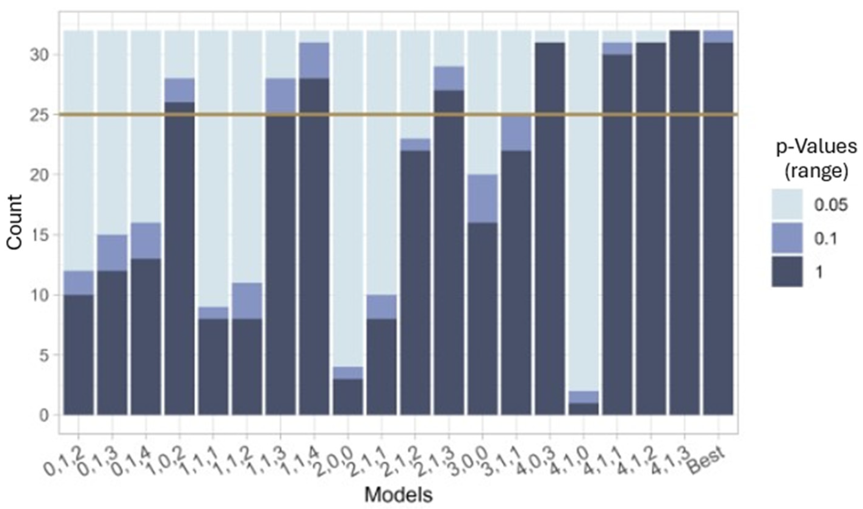
The quantity of better p-values, i.e., within the chosen significance range indicated by the upper range value (α = 0.05, 0.1, 1), is seen in Figure 1. Some of the models show that the residuals have less correlation and therefore the model accounts for more of the initial correlations across all datasets.

Figure 1.
Ljung–Box p-values from 32 datasets that are within ranges 0–0.05, 0.05–0.1, 0.1–1.
After considering p, d, and q models for both their median AIC values and the quantity of p-values that accept H0 from the Ljung–Box statistic, some strong candidates emerge. In Table 1, the median AIC values from each p, d, q model are calculated, for the top nine options (more than 25 out of 32 datasets indicated by the solid line in Figure 1) with the most p-values of the residuals being greater than 5%.

Table 1.
Median AIC values for the models with the most acceptable p-values.
Using this information as a basis, four possibilities establish themselves. The first option is to choose an ARIMA (best individual), which has the lowest median AIC and has 31 p-values above 0.05; however, it means defining the ARIMA order for every dataset rather than having a model for all shredder settings. Second, select the ARIMA (2,1,3); this has the lowest AIC and 27 p-values above 0.05 and is a model for all shredder settings. As a third option, an ARIMA (1,1,3) can be considered; this model has the second lowest median AIC, 25 p-values above 0.05, and works for all shredder settings. The fourth option is an ARIMA (1,1,4); it has the second lowest median AIC, 28 p-values above 0.05, and works for all shredder settings. For the sake of this study, the forecasting will be performed with the ARIMA (1,1,4) since its p-values are high and the AIC is as good as the individual fitting, while having the same number of parameters as option ARIMA (2,1,3). However, forecasting with the other models is also an option.
The original data have a significantly non-normal distribution, based on some trend and a cut off after some lags. Taking the first difference of the datasets results in a non-normal mean around 0, with strong correlations seen in the ACF and PACF plots up to lag 2 and 4, respectively (c.f. Figure S3 in the Supplementary Material). The residuals of the ARIMA model are tested for normal distribution and correlations using the Shapiro–Wilk test and the Ljung–Box test, which gave back consistent results for no correlation and non-normal distribution (31 out of 32 datasets). Therefore, the forecasting with the models is performed considering these conditions.
2.3. Coefficients
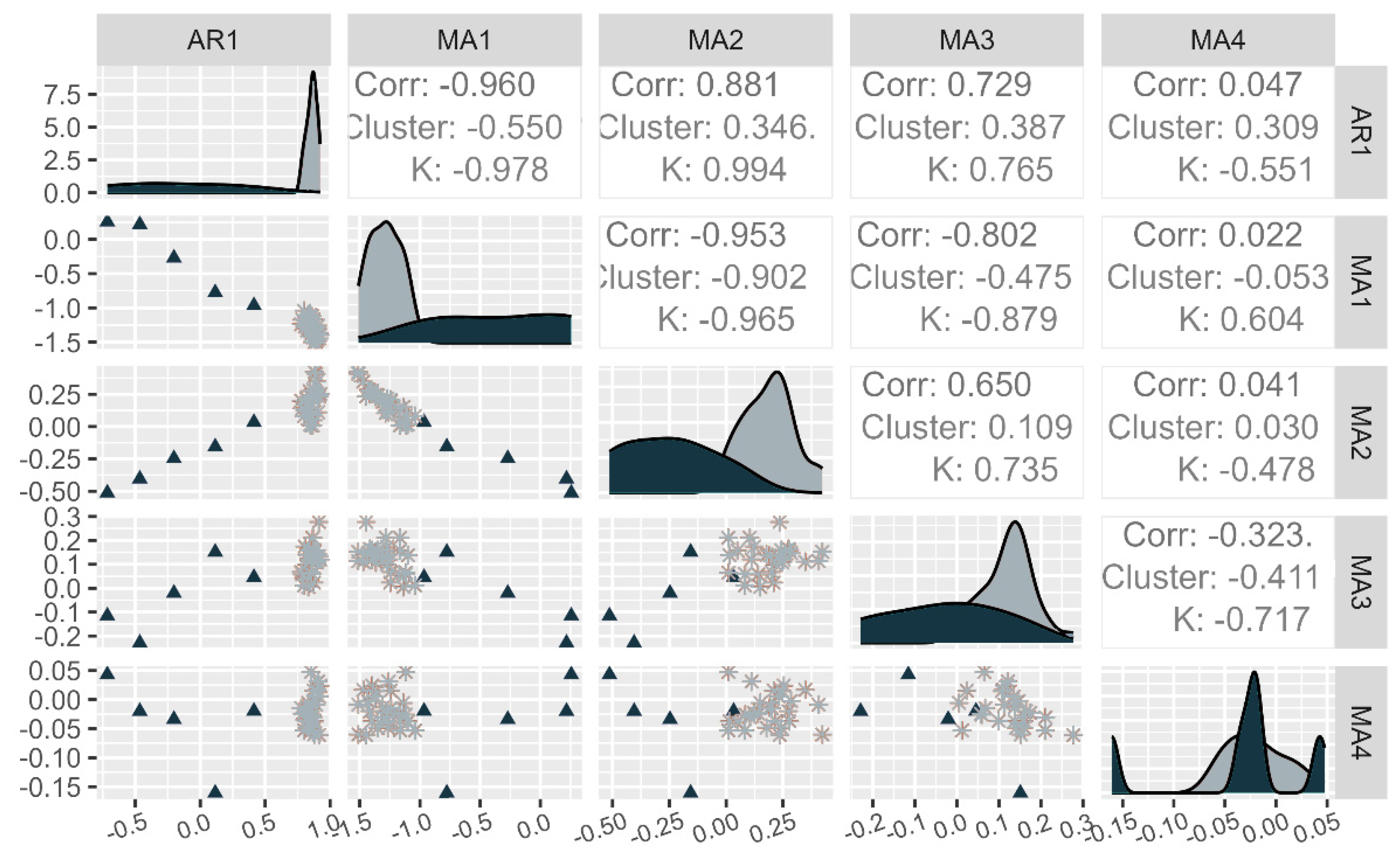
After the PCA of the coefficients resulted in a grouping of 27 datasets except for five outliers, a simple pairs plot was used to ensure the five individual outliers are the only outliers and see how wide the variance of the remaining group was across all five dimensions (coefficients AR(1)…MA(4)). The results of the pairs plot were that the datasets K02, K04, K06, K07, and K24 were the outliers and the others are grouped in limited range with a width for the AR(1) = 0.25, MA(1) = 0.5, MA(2) = 0.44, MA(3) = 0.3, MA(4) = 0.11. The outliers could not be grouped in any particular way and were from multiple shredder settings. The individual pairs plots can be seen in Figure 2 and additional figures are available in the Supplementary Material. The dataset K06 is close to the cluster, except in the AR1 dimension.
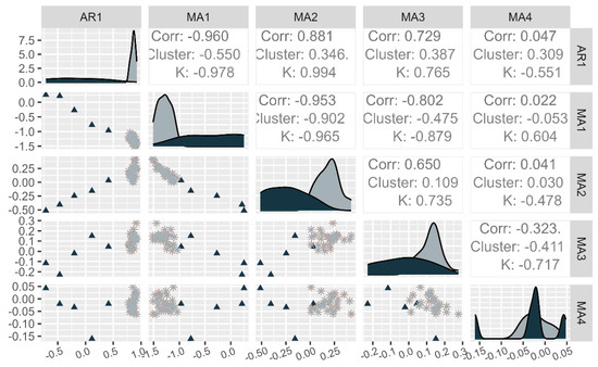
Figure 2.
Pairs plot of coefficients from ARIMA (1,1,4) outliers—triangles, cluster—stars.
2.4. Prediction Quality
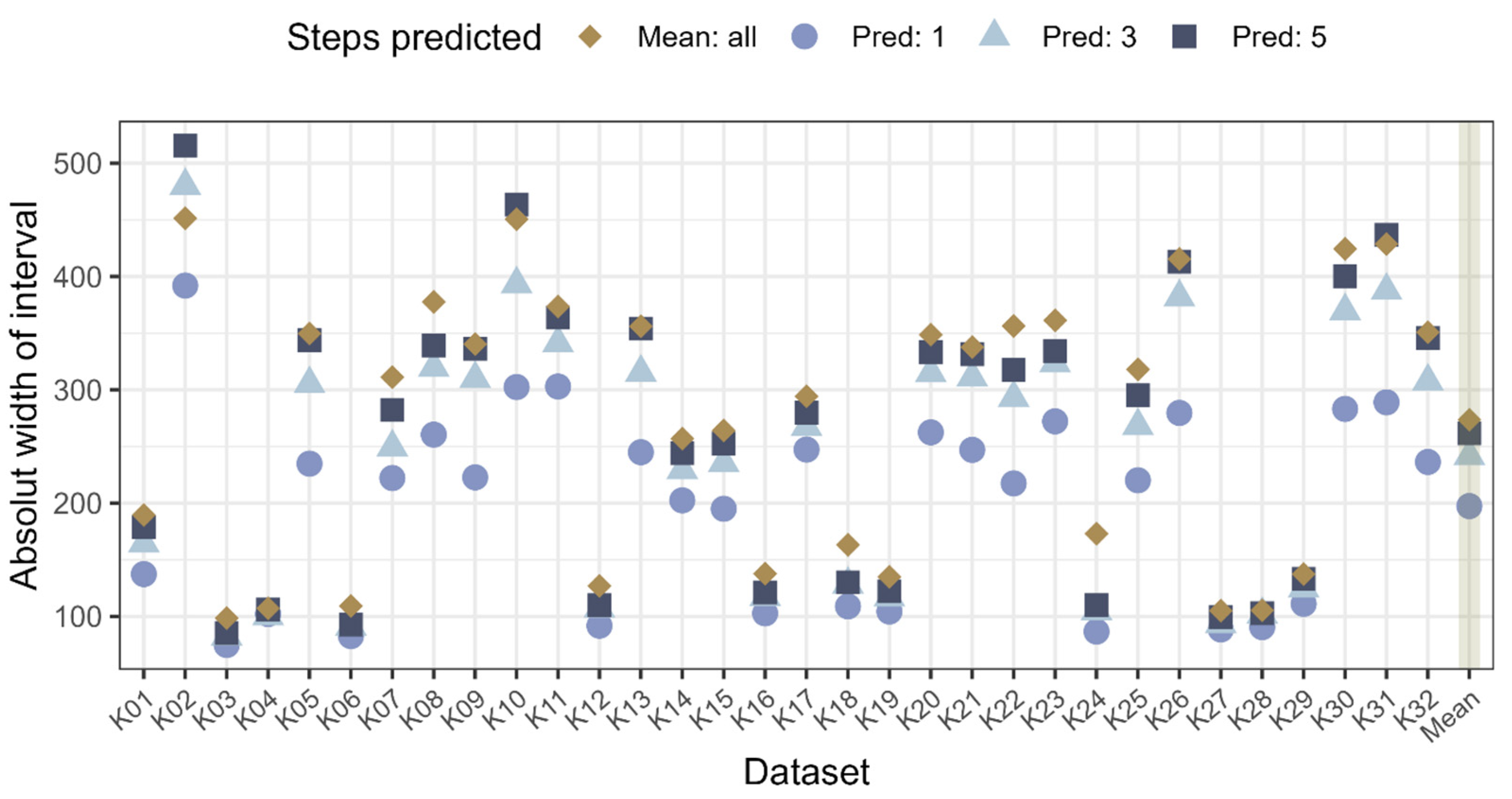
The confidence interval for the next predictions is used to compare how well the predictions perform for different prediction horizons (here, the prediction horizons are selected for one, three, and five steps) and the chosen benchmark. In Figure 3, the absolute width of the confidence intervals is displayed. It can be seen that the group with the V shaped cutting tools (lower AIC bulge: K03, K04, K06, K12, K16, K18, K19, K24, K27, K28, K29) have significantly more narrow prediction intervals, as well as the benchmark having narrower intervals compared to the F and XXF cutting tools (upper AIC bulge).
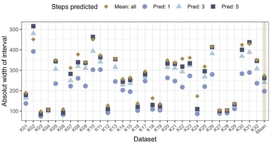
Figure 3.
ARIMA forecasting confidence interval for next one, three, and five steps with absolute values (dataset K01-K32) and mean of prediction width across all datasets (highlighted with shading on the right side of the diagram).
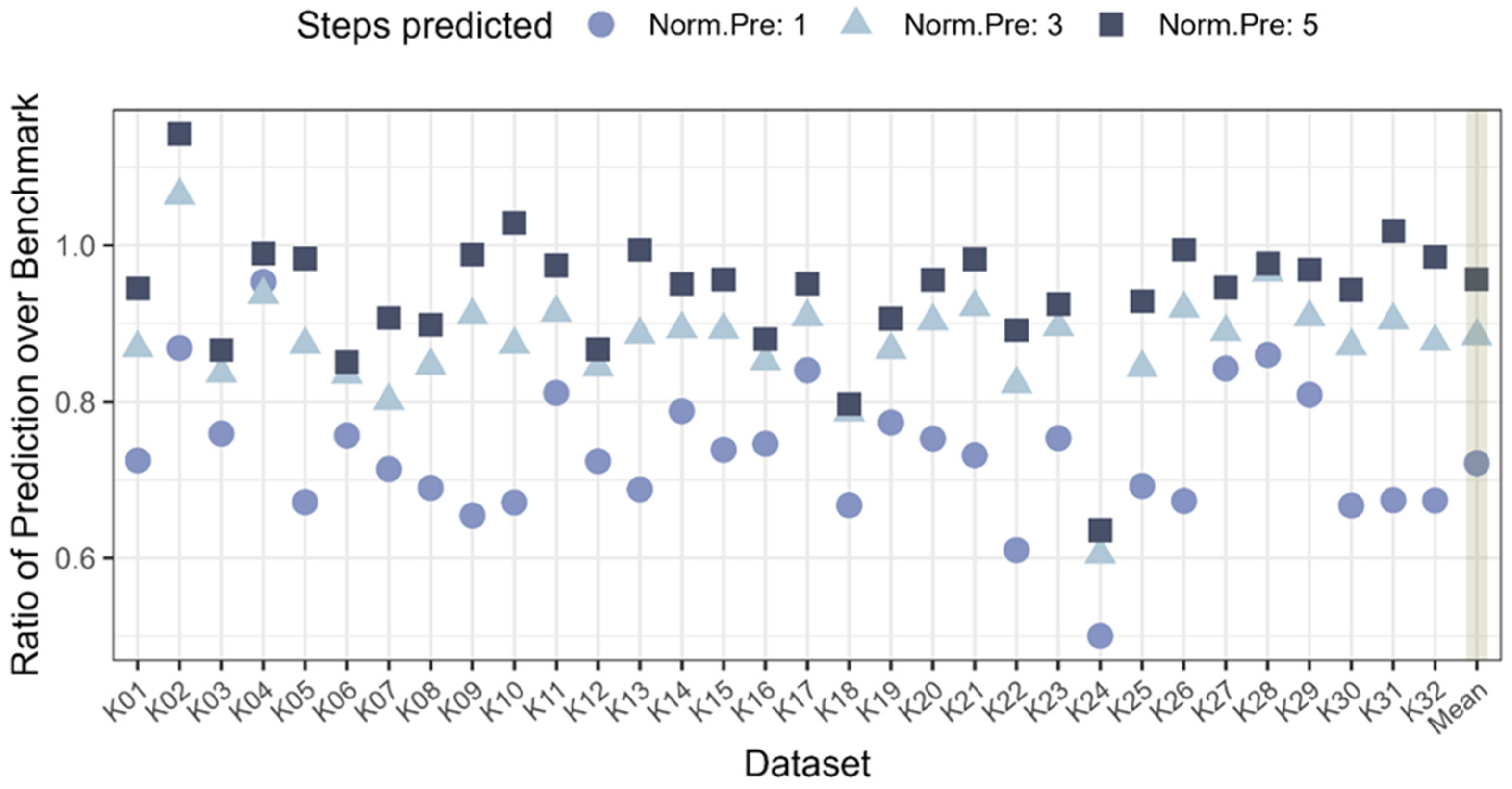
A better comparison for the relative improvement of the confidence intervals across the datasets is given in Figure 4. This gives a clearer picture of how well the model performs compared to the benchmark, as the ratio for the ARIMA model tends to be between 0.6 and 1, thus indicating an improvement of up to 40% for a one-step ahead prediction. The average of all the ratios across the 32 datasets is Pred.1: 0.72, Pred.3: 0.88, Pred.5: 0.96. This shows that on average the improvement for the ARIMA prediction is significant for one step ahead but is all but diminished by five steps ahead and seems to follow the square root prediction width increase (R = 0.9997 for y = 0.7206 × 0.1794), which would be expected for a prediction using the previous variance as a measure for future values.
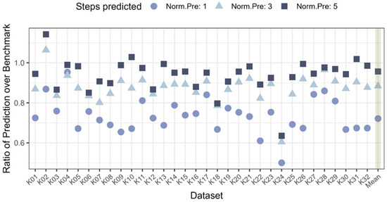
Figure 4.
Ratio of interval from ARIMA prediction over benchmark, confidence intervals of all data sets and the mean (highlighted with shading on the right side of the diagram).
The final comparison to provide a more robust evaluation is performed using the ARIMA prediction with a moving training data history. These are calculated for each of the 32 datasets, and a mean across all the values is taken for estimating the overall effectiveness of the method. The training data are presented as a moving block that is updated with the actual data coming in over time, and the prediction is made for the next value and the fifth next value for 30 consecutive data blocks (at 2 s per data point it is a time frame of 60 s, across which the training data block is shifted). The result for 30 such training data shifts is shown in Figure 5. This illustrates that the distributions for all three forecasting types have several similarities and also display the same trend of the median interval width increasing towards higher prediction horizons, yet still remaining below the benchmark value. Therefore, the better performance of the ARIMA (1,1,4) model for short-term predictions up to five steps (or 10 s) over the basic benchmark is demonstrated.
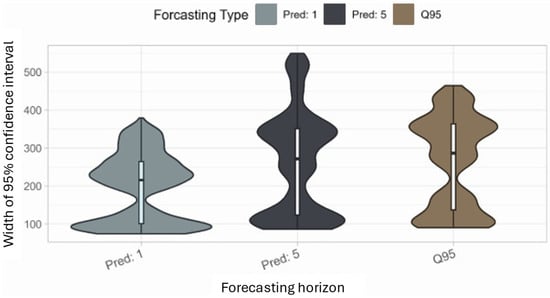
Figure 5.
Distribution of confidence width for 30 different training datasets across 32 shredder settings.
The application of this prediction for the control loop is limited since, at a prediction horizon of five steps ahead with a step time of 2 s, this means that the prediction quality of 10 s ahead is only 5% better than the quantile range across all previous values. The increased prediction quality at one step ahead is significant, but only gives a 2 s reaction time for the control loop which is too short for the change in shaft rotation speed to show an effect on the output material stream, considering that it requires approximately 1 s for the shaft rotation speed to change after the command is given for the speed change and the material also takes some seconds from exiting the shredder compartment to arriving at the volume measuring unit.
The forecast horizon is therefore limited to a maximum of 10 s with ARIMA time series modeling. Using alternative forecasting methods, e.g., the Long Short-Term Memory (LSTM) neural network model proposed by [20], could possibly reveal a higher forecasting horizon since the underlying correlations are present and can be exploited for models.
3. Discussion
This study has shown the possibility of a short-term prediction of the volume flow with a 35% smaller 95% confidence interval over a simple benchmark prediction method. This improved prediction method shows that there are some correlations in the volume flow of the shredder output stream that can be taken advantage of. However, the effect seems to be limited to a prediction horizon of only 10 s. This significantly reduces the application in a control loop suggested by [15]. In order to realize a dynamic control of a shredder, as described in [15], based on the output volume flow of a shredder, more complex models must be used to predict a longer period of time. Furthermore, the data could be obtained at an earlier position on the shredder and not generated by the volume flow sensor positioned on the discharge conveyor. Ref. [21] describes an approach for determining the volume flow by an indirect estimation of the volume throughput based on machine parameters such as drum speed and drum torque. If this potentially results in a more accurate measurement or at least a time advantage, it could provide a means of obtaining data for control, and the prediction of material composition could be made for a shorter period of time. Furthermore, other sensor technologies, or a combination of sensors (sensor-fusion), could lead to better results in data gathering and help to predict the volume flow. For example, a sensor or camera for the filling level in the shredder could provide additional information; recognizing the material composition would allow for conclusions to be drawn about the shredding behavior and further the output flow.
4. Materials and Methods
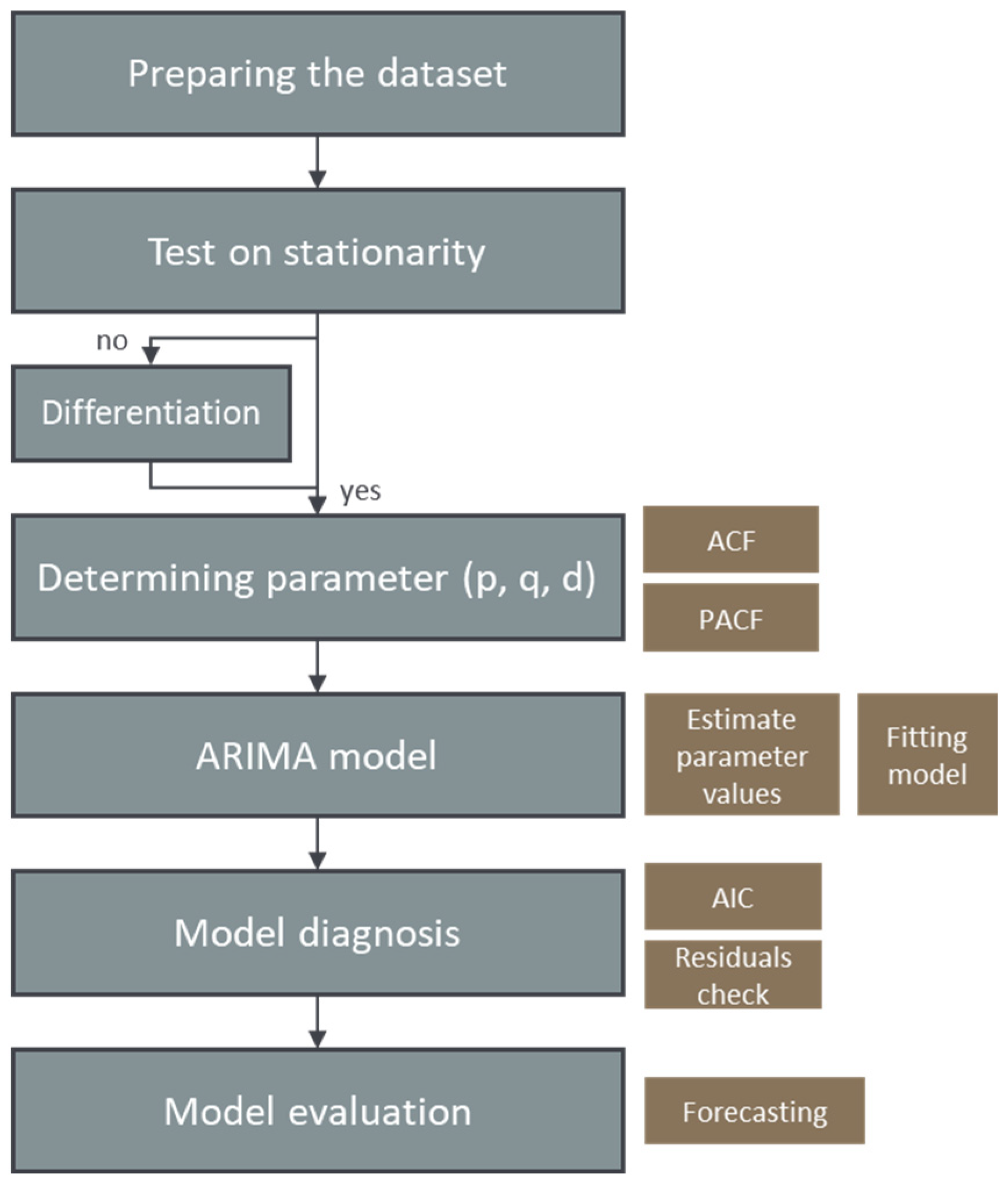
To describe the output volume flow of a shredder, time series analyses are made, which are to be described by means of a suitable ARIMA model to predict future sensor measurements based on previous knowledge. The datasets discussed in the following come from experimental runs described in [13]; in total, there are 32 datasets from 32 test runs. Details can be found in the original publication, but the following section gives a short overview of the most important data. Mixed commercial waste was comminuted by a shredder and, in addition to other data, volume flow data have been recorded. A laser triangulation measurement was used for determining the volume flow; the values were updated every 2 s, representing the arithmetic mean of the volume flow during this time. The settings on the shredding machine (gap width, shaft speed, and the cutting tool) have been changed for each test run. The cutting tools are divided into three groups, type F, type XXF, and type V; the technical details of the geometries are tabulated and described in [13]. The gap width is described as a percentage of the maximum aperture and ranges from 0 to 100%; 11 factor levels are possible here, as the changeover takes place in 10% steps. The shaft speed is described as a percentage of the maximum rotation frequency (31 rpm), ranging from 60 to 100%, and could be varied in 10% steps, resulting in five possible factor levels. The experiments were performed according to a DoE [13]. The data are analyzed based on the “Run planned” numbering, to be found in the supplementary material of [13]. The datasets, as a part of preprocessing, are cleaned up and filtered for further processing in R, as well as typical intervals between significant changes in the measurement values are determined. The data are reduced by selecting only representative rows based on the change in values, to avoid using data points multiple times. Figure 6 is intended to support the steps described below, which were taken to find a suitable ARIMA model used in these investigations for forecasting.
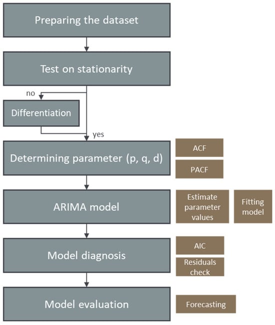
Figure 6.
Method graphic to illustrate the steps for creating an ARIMA model for time series analysis.
4.1. Time Series Analysis
Time series analysis is a statistical method in which data points collected at regular intervals are analyzed in order to examine underlying trends and to determine the correlation between observations that vary over time. The order of the data points is crucial; rearranging them could lead to a loss of meaningful insights or distort the interpretation. In addition, time series analysis often requires a large dataset to maintain the statistical significance of the results. This allows analysts to filter out the “noise” and ensure that the patterns observed are not just outliers, but statistically significant. To predict future values based on previously observed data, a time series forecasting model is used [22,23].
4.2. ARIMA Models
ARIMA models are among the most commonly used approaches for time series forecasting by describing the autocorrelations in the data [18]. The ARIMA model is a statistical analysis model that utilizes time series data either to understand the dataset better or to predict future trends, or to predict the current value from a series of past values. Equation (1) gives the mathematical definition of the ARIMA model. The following text passage should serve as additional information to the mathematical description. The Autoregressive (AR) part can predict future values based on p historical values, where p is the number of steps into the past. The Integration (I) is performed to make the time series stationary, the component d indicates the number of differentiations. The differentiated values are reintegrated after the model has been created to form a model for the original data series. The Moving Average (MA) model of order q takes errors of the predictions to form the observed data [19,23]. The current value of the series, xt, is described by the AR(p), the MA(q), and the I(d) part. The AR part is a series xt defined by p past values xt−1, …, xt−p, and after each value is multiplied by a corresponding coefficient φt, and wt (the white noise) is added to the sum. The moving average assumes a linear combination of the white noise wt to form the observed data, which are multiplied by the coefficients θt [23].
Equation (1): ARIMA Model of Order p, d, q [23].
Many of the methods to fit and apply an ARIMA model require the dataset to be stationary. This means the mean and variance are constant over time. If necessary, differentiation of the dataset must be applied to achieve stationarity. Stationarity is tested for via the presence of a unit root, which results in a time series variance or mean to change over time, and is tested using the Augmented Dickey–Fuller (ADF) test and the Kwiatkowski–Phillips–Schmidt–Shin (KPSS) test [24,25]. The following methods are applied under the assumption of stationarity.
An ARIMA model is determined to have an optimal fit to the underlying data. The aim of this identification is to select the three parameters p, q, and d of the time series as effectively as possible. This can be performed with the help of ACF (autocorrelation function) and PACF (partial autocorrelation function). The ACF indicates the duration and presence of a temporal relationship in the material flow. In the study [15], the dynamic control of the shredder relies on the material-based relationship of the ACF. The joint consideration of ACF and PACF plots can aid in the model selection of an ARIMA model for investigating time series [23]. In time series analysis, ACF and PACF plots are two of the most important tools for identifying the underlying structure of a time series. The ACF plot shows the correlation of a time series with itself at various time lags, while the PACF plot shows the correlation of a time series with itself at various lags after removing the effects already explained on previous lags. The ACF plot can be used to determine the order of the MA part of an ARIMA model. The PACF plot can be used to determine the order of the AR part [23]. Furthermore, the ACF and PACF plots are used to identify trends, structures, and seasonal patterns in data. For example, significant peaks in certain lags indicate seasonal patterns. The ACF and PACF are calculated using the R stats package (version 4.2.1) [26].
After determining the appropriate parameters (p, q, and d) for the model, the parameter values are estimated using common estimation methods. After fitting the model to the data, it is important to perform a review to assess the appropriateness of the model and identify areas for improvement, which can be performed using the Akaike Information Criterion (AIC). It is a measure of how well a statistical model represents the data, taking into account both the quality of fit and the model’s complexity. In the context of ARIMA models in time series analysis, AIC is often used to select the best ARIMA model. When choosing between different ARIMA (p, d, q) models with different values for p, d, and q, the model with the lowest AIC value is selected [27,28]. In this study, the AIC value is used for model selection, which is calculated with the forecast-package from the R-Library software [19,27].
4.3. Model Evaluation
The first steps after deciding on the model involve cleaning up the datasets. In this context, this means removing time sections where there was no material available to the shredder, and ensuring that each measurement is only represented once in the datasets. Secondly, time plots were checked by using ACF and PACF plots for any trends, periodic or seasonal effects, or anomalies. Next, the gathered information from the ACF and PACF is used to begin estimating the range of p, d, and q ARIMA parameters. Then the R-simulation for the range of p, d, q values is run, and the AIC values from the various model orders are calculated. Finally, the results are evaluated, and a model to proceed with for the prediction of the next output datapoints is chosen.
The AIC values are not the only criteria to consider for the model fit. Another measure of how well the model fits the data is whether the residuals after fitting the model to the data are distributed normally and have no correlations. This can be tested using the Ljung–Box statistic, of which the Null Hypothesis (H0) is “The data is uncorrelated”. Therefore, it is desirable to have p-values above the chosen significance level since H0 should be accepted [29,30]. The Shapiro–Wilk test is used to evaluate whether a dataset is normally distributed (Null Hypothesis H0) or is not normally distributed (Alternative H1) and is calculated using the R stats package 4.2.1 [31]. If the data cannot be assumed to be normally distributed, as is the case with these 32 datasets, but does not show significant correlations, and the variance can be assumed to be constant, a forecast is performed using the bootstrapping method. This forecasting method uses previous residuals from the training data to randomly use the residuals as an error term for the next predicted value. The applied function in R uses Moving Block Bootstrap (MBB), which is best at preserving any correlations [27,32,33].
4.4. Coefficients
After choosing an order for the ARIMA model, the calculated coefficients (i.e., AR(1)…MA(4)) for each dataset are saved, and the values can be compared to each other. The coefficients for each dataset model are calculated by using the first part of the respective dataset as training data to which the ARIMA model with individual coefficient values is fitted. This way, the last part of the time series data can be used as test data for the prediction part of the process. The idea to check for clusters and similarities within the coefficient values was tested using the principal component analysis (PCA). This is a method to reduce the dimensionality of a complex dataset and transform it onto a new coordinate system with orthogonal axes that represent the principal components and capture the most variance [34].
4.5. Prediction Quality and Analysis of Residuals
A prediction for the next value (Pred 1) and the fifth next value (Pred 5) is made using the chosen ARIMA model. When using datasets for prediction purposes, the time series sets are split into two parts to create a dataset where the prediction can be tested. This is performed by using the first part of the data as training data for the model to be fitted and the second part, or testing data, to compare the model predictions to the recorded historical data. The training data of the 32 datasets are used while taking into account the non-normality of the data by using the bootstrapping method. The values for Pred 1 and 5 are predicted by using the ARIMA equation, see Equation (1), with its coefficients and inserting an error term for the next value based on the residual error from the training data. The assumption is that the distribution of the future residuals will be similar to the distribution of the previous residuals. Using the calculated prediction widths of the confidence interval for the next five values to compare them against the chosen benchmark of predicting the median value of the training data and placing a 95% quantile range over it, i.e., the range is Q2.5–Q97.5. This prediction method is very basic but describes 95% of the data variance, and so the ARIMA model must perform better than this chosen benchmark. By using the 95% quantile range rather than ±1.96×σ, the range of the 95% confidence interval for a normal distribution, the prediction is not dependent on the assumption of a normal distribution, which is not granted in this application. The width of the ARIMA prediction interval is calculated by R using the MBB from the forecast Package as described in [27,32].
5. Conclusions
Throughput and, more specifically, throughput fluctuations, are a relevant issue in mechanical waste treatment processes. Smoothing the fluctuations could lead to better results in terms of processing the material (e.g., mixed solid waste) in the individual machines and overall, to better material qualities (e.g., if subsequent machines are not overloaded). As can be seen in [15], a simple implemented control of the throughput to reduce the fluctuations at the shredder output volume flow did not produce a positive result. For this reason, this study focused on a solution that could predict the volume flow and thus give the control system more time to react to the material flow. In order to be able to predict the volume flow, time series analyses were carried out using ARIMA models. One of several possible ARIMA models was selected (ARIMA (1,1,4)) and used to make a prediction. It was possible to predict for 10 s, still providing significant results. However, this time period is slightly not long enough to implement a dynamic control; alternative prediction methods could still be tested to predict for a longer time horizon. Nevertheless, time series analysis also works in the waste sector and could therefore still provide good insights in terms of dynamic control.
Supplementary Materials
The following supporting information can be downloaded at: https://www.mdpi.com/article/10.3390/recycling10030083/s1, Figure S1: AIC comparison for all the best ARIMA models for order AR(p), I(d), MA(q) across all 32 datasets. Figure S2: Autocorrelation function (ACF)–left, and Partial Autocorrelation function (PACF)–right of differenced K31 (run planned). Figure S3: ARIMA Residual density, Normal density distribution–orange line, Density distribution of Residuals from ARIMA (1,1,4)–blue area. Figure S4: ARIMA (1,1,4) coefficients. Figure S5: Prediction based on ARIMA (1,1,4) Model and Mean of All (MoA) benchmark with 95% confidence Intervals.
Author Contributions
Conceptualization, T.L. and K.K.; methodology, T.L., J.I. and K.K.; software, T.L., J.I., L.K. and K.K.; validation, T.L., J.I. and K.K.; formal analysis, T.L. and J.I.; investigation, K.K. and R.S.; resources, K.K. and R.S.; data curation, T.L., I.J., K.K. and R.S.; writing—original draft preparation, T.L. and J.I.; writing—review and editing, T.L., L.K., K.K. and R.S.; visualization, T.L., L.K. and J.I.; supervision, R.S.; project administration, R.S.; funding acquisition, R.S. All authors have read and agreed to the published version of the manuscript.
Funding
Recycling and Recovery of Waste for Future (project nr. 882512) is a COMET Project within the COMET–Competence Centers for Excellent Technologies Programme and funded by BMK, BMAW and the federal state of Styria. COMET is managed by FFG. The Center of Competence for Recycling and Recovery of Waste 4.0 (acronym ReWaste4.0) (contract number 860 884) under the scope of the COMET–Competence Centers for Excellent Technologies–financially supported by BMVIT, BMDW, and the federal state of Styria, managed by the FFG.
Data Availability Statement
The raw data supporting the conclusions of this article will be made available by the authors on request, the data presented in this study are available on request from the corresponding author due to as it is partly confidential data.
Conflicts of Interest
The authors declare no conflicts of interest.
Abbreviations
The following abbreviations are used in this manuscript:
| ACF | Autocorrelation function |
| ADF | Augmented Dickey–Fuller |
| AIC | Akaike Information Criterion |
| Approx. | Approximately |
| ARIMA | Auto-Regressive Integrated Moving Average |
| EU | European Union |
| i.e., | Id est (that is) |
| KPSS | Kwiatkowski-Phillips-Schmidt-Shin |
| LSTM | Long Short-Term Memory |
| MBB | Moving Block Bootstrap |
| PACF | Partial autocorrelation function |
| PCA | Primary Component Analysis |
| Pred 1 | Prediction for the next value |
| Pred 3 | Prediction for the 3rd next value |
| Pred 5 | Prediction for the 5th next value |
| Q | Quantile |
References
- European Commission. Communication from the Commission to the European Parliament, the Council, the European Economic and Social Commitee and the Commitee of the Regions: A New Circular Economy Action Plan. For a Cleaner and More Competitive Europe, Brussels. 2020. Available online: https://eur-lex.europa.eu/legal-content/EN/TXT/?qid=1583933814386&uri=COM:2020:98:FIN (accessed on 17 December 2024).
- Federal Ministry Republic of Austria Climate Action. Environment, Energy, Mobility, Innovation and Technology, Austria on the Path to a Sustainable and Circular Society; The Austrian Circular Economy Strategy: Vienna, Austria, 2022.
- Sarc, R.; Curtis, A.; Kandlbauer, L.; Khodier, K.; Lorber, K.E.; Pomberger, R. Digitalisation and Intelligent Robotics in Value Chain of Circular Economy Oriented Waste Management—A Review. Waste Manag. 2019, 95, 476–492. [Google Scholar] [CrossRef]
- Fatimah, Y.A.; Govindan, K.; Murniningsih, R.; Setiawan, A. Industry 4.0 based sustainable circular economy approach for smart waste management system to achieve sustainable development goals: A case study of Indonesia. J. Clean. Prod. 2020, 269, 122263. [Google Scholar] [CrossRef]
- Antikainen, M.; Uusitalo, T.; Kivikytö-Reponen, P. Digitalisation as an Enabler of Circular Economy. Procedia CIRP 2018, 73, 45–49. [Google Scholar] [CrossRef]
- Moreno, M.; Charnley, F. Can Re-Distributed Manufacturing and Digital Intelligence Enable a Regenerative Economy? An Integrative Literature Review. In Sustainable Design and Manufacturing 2016; Springer: Cham, Switzerland, 2016; pp. 563–575. [Google Scholar] [CrossRef]
- Borchard, R.; Zeiss, R.; Recker, J. Digitalization of waste management: Insights from German private and public waste management firms. Waste Manag. Res. 2022, 40, 775–792. [Google Scholar] [CrossRef] [PubMed]
- Sarc, R.; Curtis, A.; Khodier, K.; Koinegg, J.; Ortner, M. Digitale Abfallwirtschaft. Digital Waste Management; Recy & DepoTech: Leoben, Austria, 2018. [Google Scholar]
- Kurniawan, T.A.; Avtar, R.; Singh, D.; Xue, W.; Othman, M.H.D.; Hwang, G.H.; Iswanto, I.; Albadarin, A.B.; Kern, A.O. Reforming MSWM in Sukunan (Yogjakarta, Indonesia): A case-study of applying a zero-waste approach based on circular economy paradigm. J. Clean. Prod. 2021, 284, 124775. [Google Scholar] [CrossRef] [PubMed]
- Kurniawan, T.A.; Othman, M.H.D.; Liang, X.; Goh, H.H.; Gikas, P.; Kusworo, T.D.; Anouzla, A.; Chew, K.W. Decarbonization in waste recycling industry using digitalization to promote net-zero emissions and its implications on sustainability. J. Environ. Manag. 2023, 338, 117765. [Google Scholar] [CrossRef] [PubMed]
- Gursch, H.; Körner, S.; Thaler, F.; Waltner, G.; Gastner, H.; Rinnhofer, A.; Oberwinkler, C.; Meisenbichler, R.; Bischof, H.; Kern, R. Digitalisation of Refuse Sorting with Image Recognition and Time Series Analysis; Recy & DepoTech: Leoben, Austria, 2022. [Google Scholar]
- Feil, A.; Pretz, T. Ungenutzte Potenziale in der Abfallaufbereitung. Unused Potentials in Waste Treatment; Recy & DepoTech: Leoben, Austria, 2018. [Google Scholar]
- Khodier, K.; Feyerer, C.; Möllnitz, S.; Curtis, A.; Sarc, R. Efficient Derivation of Significant Results from Mechanical Processing Experiments with Mixed Solid Waste: Coarse-Shredding of Commercial Waste. Waste Manag. 2021, 121, 164–174. [Google Scholar] [CrossRef]
- Küppers, B.; Seidler, I.; Koinig, G.R.; Pomberger, R.; Vollprecht, D. Influence of throughput rate and input composition on sensor-based sorting efficiency. Detritus 2020, 9, 59–67. [Google Scholar] [CrossRef]
- Lasch, T.; Imhof, J.; Sarc, R.; Khodier, K. Development of a method for shredder characterisation and dynamic control of the output material stream. J. Sustain. Dev. Energy Water Environ. Syst. 2024, 12, 1–10. [Google Scholar] [CrossRef]
- Araghinejad, S. Time Series Modeling: Data-Driven Modeling: Using MATLAB® in Water Resources and Environmental Engineering; Springer: Dordrecht, The Netherlands, 2014. [Google Scholar] [CrossRef]
- Chatfield, C. Time-Series Forecasting; Chapman & Hall/CRC: Boca Raton, FL, USA, 2000. [Google Scholar] [CrossRef]
- Hyndman, R.J.; Athanasopoulos, G. Forecasting: Principles and Practice; Otexts Online Open-Access Textbooks: Melbourne, Australia, 2021. [Google Scholar]
- Hyndman, R.J.; Khandakar, Y. Automatic Time Series Forecasting: The forecast Package for R. J. Stat. Softw. 2008, 27, 1–22. [Google Scholar] [CrossRef]
- Cubillos, M. Multi-Site Household Waste Generation Forecasting Using a Deep Learning Approach. Waste Manag. 2020, 115, 8–14. [Google Scholar] [CrossRef]
- Feyerer, C.; Khodier, K.; Lasch, T.; Pomberger, R.; Sarc, R. Indirect Estimation of the Volumetric Throughput Performance in Shredding of Solid Waste. Clean Technol. 2025. [Google Scholar]
- Fahrmeir, L.; Heumann, C.; Künstler, R.; Pigeot, I.; Tutz, G.; Fahrmeir, L.; Heumann, C.; Künstler, R.; Pigeot, I.; Tutz, G. Statistik: Der Weg zur Datenanalyse, 9th ed.; Springer: Berlin, Germany, 2023; pp. 553–578. [Google Scholar] [CrossRef]
- Shumway, R.H.; Stoffer, D.S. Time Series Analysis and Its Applications: With R Examples; Springer: Cham, Switzerland, 2017. [Google Scholar]
- Kwiatkowski, D.; Phillips, P.C.B.; Schmidt, P.; Shin, Y. Testing the null hypothesis of stationarity against the alternative of a unit root. J. Econom. 1992, 54, 159–178. [Google Scholar] [CrossRef]
- Said, S.E.; Dickey, D.A. Testing for Unit Roots in Autoregressive-Moving Average Models of Unknown Order. Biometrika 1984, 71, 599–607. [Google Scholar] [CrossRef]
- Chambers, J.; Eddy, W.; Härdle, W.; Sheather, S.; Tierney, L.; Venables, W.N.; Ripley, B.D. Modern Applied Statistics with S; Springer: New York, NY, USA, 2002. [Google Scholar] [CrossRef]
- Hyndman, R.; Athanasopoulos, G.; Bergmeir, C.; Caceres, G.; Chhay, L.; O’Hara-Wild, M.; Petropoulos, F.; Razbash, S.; Wang, E.; Yasmeen, F. Forecast: Forecasting Functions for Time Series and Linear Models: R Package Version 8.21.1; Monash University: Melbourne, Australia, 2023. [Google Scholar]
- Newbold, P. ARIMA model building and the time series analysis approach to forecasting. J. Forecast. 1983, 2, 23–35. [Google Scholar] [CrossRef]
- Lijung, G.M.; Box, G.E.P. On a measure of lack of fit in time series models. Biometrika 1978, 65, 297–303. [Google Scholar] [CrossRef]
- Box, G.E.P.; Pierce, D.A. Distribution of Residual Autocorrelations in Autoregressive-Integrated Moving Average Time Series Models. J. Am. Stat. Assoc. 1970, 65, 1509–1526. [Google Scholar] [CrossRef]
- Shapiro, S.S.; Wilk, M.B. An analysis of variance test for normality (complete samples). Biometrika 1965, 52, 591–611. [Google Scholar] [CrossRef]
- Pan, L.; Politis, D.N. Bootstrap prediction intervals for linear, nonlinear and nonparametric autoregressions. J. Stat. Plan. Inference 2016, 177, 1–27. [Google Scholar] [CrossRef]
- Bergmeir, C.; Hyndman, R.J.; Benítez, J.M. Bagging exponential smoothing methods using STL decomposition and Box–Cox transformation. Int. J. Forecast. 2016, 32, 303–312. [Google Scholar] [CrossRef]
- Vandeginste, B.; Massart, D.L.; Buydens, L.; de Jong, S.; Lewi, P.J.; Smeyers-Verbeke, J. Chapter 31—Analysis of Measurement Tables. In Handbook of Chemometrics and Qualimetrics: Part B; Data Handling in Science and Technology; Elsevier: Amsterdam, The Netherlands, 1998. [Google Scholar]

Disclaimer/Publisher’s Note: The statements, opinions and data contained in all publications are solely those of the individual author(s) and contributor(s) and not of MDPI and/or the editor(s). MDPI and/or the editor(s) disclaim responsibility for any injury to people or property resulting from any ideas, methods, instructions or products referred to in the content. |
© 2025 by the authors. Licensee MDPI, Basel, Switzerland. This article is an open access article distributed under the terms and conditions of the Creative Commons Attribution (CC BY) license (https://creativecommons.org/licenses/by/4.0/).