1. Introduction
The battery industry is growing at an exceptional rate driven by the growing electric vehicle industry. Range and power demands from consumers are forcing the industry to develop more capable batteries. Therefore, along with new chemistries being developed, existing chemistries are continually tweaked to meet a need. These often small changes can result in large changes in the behaviour of the battery over a single cycle and/or its lifetime. To understand cell performance, extensive tests are required. These tests should reflect the usage case, both in terms of operational load and thermal conditions. Since testing is expensive and time-consuming, the battery industry looks to minimise the experimental work required during the development of any new battery pack. Numerical models provide an excellent alternative and are employed whenever there is sufficient confidence in their outputs and results.
There are different methods for modelling batteries such as physics-based models or equivalent circuit models (ECMs). Physics-based models predict the behaviour of the underlying electrochemical mechanisms through parameterisation of material properties and mathematical equations that define the electrochemistry. Equivalent circuit models predict battery performance by fitting the parameters of an equivalent circuit to experimental training datasets such that the equivalent circuit’s voltage response closely matches the voltage response from the training set [
1,
2]. ECMs are often preferred within the automotive industry because they are comparatively simpler, requiring far less computational effort compared to their physics-based counterparts, and they can be tailored to be most effective in a specific application [
3,
4]. There are three stages to developing a robust ECM: (i) equivalent circuit design, (ii) model parameterisation and (iii) model validation. Model parameterisation further splits into two stages: experiments for data collection required for parametrisation and then parameter value identification based on a fitting process of the equivalent circuit to the experimental data. The focus of this study is on the experimental techniques used for data collection for parametrisation of ECMs.
Two factors are important in developing battery models: their accuracy, which is intuitively critical given the role the model will subsequently play in battery pack development and operation, and the time it takes to develop the model. The latter is often overlooked within academia but is a critical component of success for companies looking to build battery packs; it can be prohibitively expensive to spend several months creating a battery model. Most importantly, the accuracy and speed of development of all models are affected by the experimental method [
5] and the precision of the experimental data used to parameterise these models.
With bad model parameters, it is impossible to create a good model. Moreover, the accuracy of the experimental data used for the parametrisation is temperature-dependent. The type of temperature control during testing is important as it does not just set a single temperature, but also affects the magnitude of the thermal gradients within a cell and, hence, the electrochemical behaviour. The speed at which a model can be developed depends on the type of model being developed. Fully discretised 3D equivalent circuit models (ECMs) are significantly more complex than single-node ECMs and, thus, the development time increases; this is further increased when the model is thermally coupled. Whilst the model code can be re-used, their model parameters vary for each battery. Therefore, a developer may spend considerable time creating the model, but this only needs to be conducted once. However, a full parameterisation procedure must be followed for every single physical battery the model will be used to emulate. As a result, parameterisation is a long-term bottleneck and minimising the time taken to conduct the parameterisation experiments is important.
Experimental techniques typically used for the parametrisation of ECMs are electrochemical impedance spectroscopy (EIS) [
6,
7,
8], Galvanostatic intermittent titration technique (GITT) [
9,
10,
11,
12,
13] and hybrid pulse power characterisation (HPPC) [
5,
14,
15,
16,
17]. GITT is the most common technique used by the battery industry, in part because it does not require complex cell-cycling equipment. By contrast, EIS requires expensive specialist potentiostats that are fitted with additional capability to run EIS cycles. Such potentiostats are not typically found in labs of private-sector companies [
11,
18,
19].
The purpose of this study is to present parameterisation methods that are relevant to industry and comparable to existing and widely used techniques. HPPC has a series of pulses applied at different SoC intervals. The charge pulses are followed by a discharge pulse and are repeated at different pulse magnitudes at every SoC but the pulses generate heat and cause errors in ECM parameters and, therefore, HPPC is not commonly used in industry in comparison to GITT. Therefore, GITT was used as the benchmark throughout the presented investigation. The procedure combines constant current discharge pulses (i.e., current loading the battery) followed by long rest periods where the electrochemical relaxation of the cell is monitored and recorded.
However, GITT is not perfect—there are considerable limitations associated with the procedure. As previously introduced, the time–cost of parameterisation is an important consideration for private-sector companies, and in this regard GITT is limiting. The time to complete a GITT procedure can vary, depending on the accuracy of the experimental data required. One set of GITT experiments lasting up to 80 h are commonly reported [
11,
13]. These include long rest times which are essential to allow the cell to return to chemical and thermal equilibrium between current loading pulses [
20,
21]. When parameterising a thermally coupled ECM that operates over a range of currents, this time is multiplied by the number of temperatures and C-rates experiments should be conducted. Hence, it can easily take many months to collect the full suite of data required for complete parameter extraction and model accuracy.
This study presents a novel accelerated model parameterisation procedure (AMPP) to meet the clear need of reduced parameterisation time. The performance of the AMPP was assessed against the GITT benchmark through parameterisation of ECMs which are then compared directly via the WLTP (worldwide harmonised light vehicle test procedure) driving cycle. All experiments were conducted at two different temperatures, 10 °C and 25 °C. This facilitated the assessment of the parameterisation procedure performance in ambient and sub-ambient conditions, where battery resistance will be higher and sensitivity to temperature change is more significant. This point leads to the second key objective of the investigation—evaluating the suitability of climate chamber control compared with high-precision conductive thermal control when GITT and AMPP are used for ECM parameterisation experiments. Misrepresentation of battery temperature leads to error ridden results, since temperature affects the electrochemical response of any battery [
5,
8,
11,
22]. Isothermal conditions are typically desired during battery parameterisation, but seldom achieved in climate chambers given the limitations associated with convective cooling. To demonstrate the influence of good temperature control on accurate experimental data, a comparison of two temperature control methods is made for the AMPP technique: a climate chamber and a Peltier element control system. In this study, the Peltier element control system will be referred to as the ICP (isothermal control platform). The ICP uses Peltier elements to control the temperature of cooling plates which sandwich the cell; the whole setup is then submerged in oil to extract heat from the Peltier elements [
13].
2. Modelling and Parametrisation Method
2.1. Model and Parameter Extraction
The sole focus of this paper is on the experiments for the parameterisation. Hence, for the model selection and parameter extraction, care was taken to ensure that no new methodology was introduced and existing methodology from the literature was used.
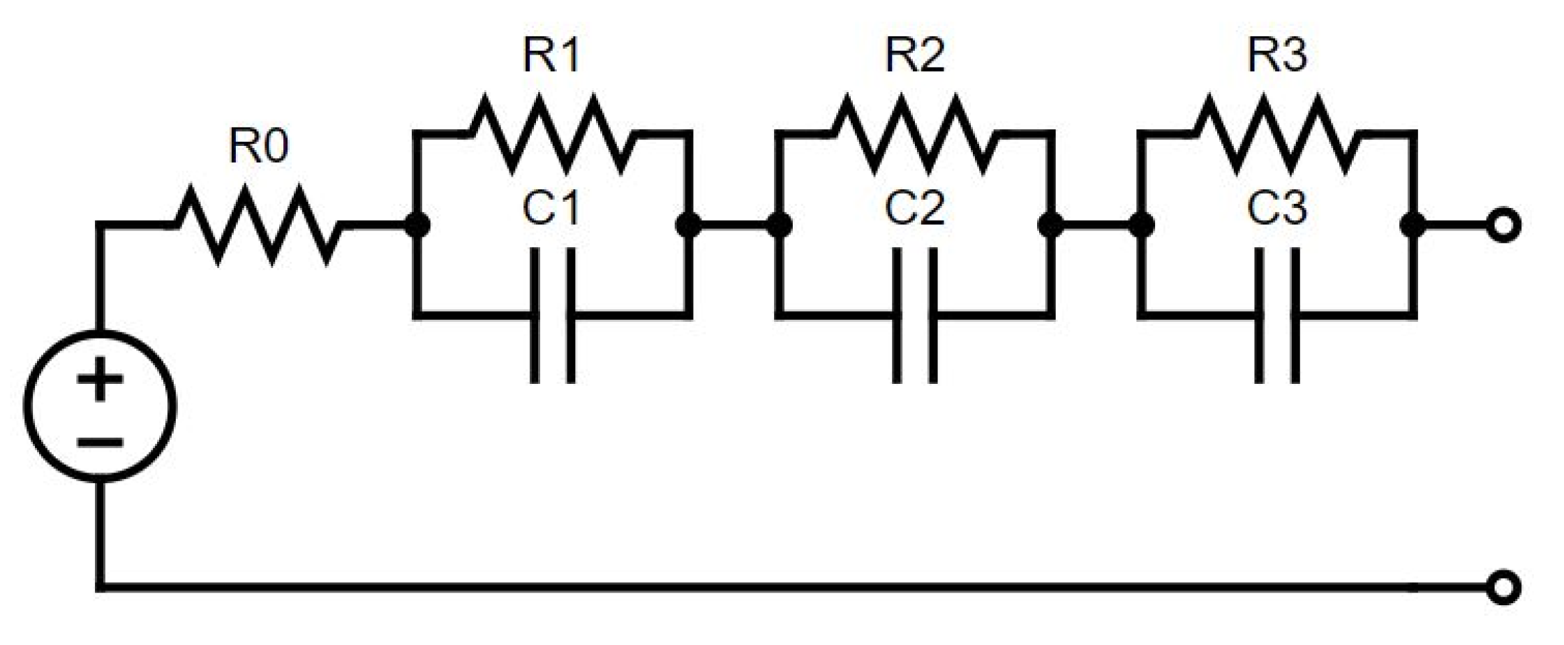
Each set of experimental data for parameterisation was used to extract a unique set of ECM parameters (
Figure 1), bounded by limits set for the investigation. In all cases, the data were used to parameterise a simple equivalent circuit containing three resistor–capacitor (RC) parallel pairs in series with each other and a series resistor to represent the ohmic resistance of the cell [
11]. The time constant, τ = RC, of each RC pair was set to τ
1 = 2.1 s, τ
2 = 35 s and τ
3 = 350 s. These values are typical for the 622NMC-graphite chemistry (LiNi
0.6Mn
0.2Co
0.2O
2) present in our test cell [
12]. The time constants were held constant to remove a degree of freedom from the parameter extraction process, which would add variability to the subsequent performance of the parameterised ECMs. Fixing the time constants does not favour GITT over AMPP or vice versa; it allows us to isolate resistive response during the completion of each procedure, which in turn yields a more robust comparison process, increasing confidence in quoted quantities within the confinements of the investigation.
The parameter extraction process was built around the MATLAB optimisation toolbox, employing methods developed by Jackey et al. [
23]. An identical procedure was followed for each unique set of parameters, in order to normalise results and reduce procedural error from one set to the next. Parameters were extracted for specific state-of-charge (SoC) windows. The SoC windows used by Li et al. [
12] were followed in this study, such that 2% SoC windows were employed below 20% SoC and above 90% SoC. From 20–90% SoC, the window size was 4% SoC.
2.2. Parametrisation of ECM
A 20 Ah NMC-622 pouch cell was used to conduct the GITT and AMPP experiments (
Table 1). Both experiments were conducted on the same physical cell. For the AMPP, a Biologic HCP-1005 Potentiostat (Seyssinet-Pariset, France) was used, with a maximum allowable current of 100 A. For the GITT, a 120 A Maccor model Series 4000 battery cycler (Tulsa, OK, USA) was used.
2.2.1. Galvanostatic Intermittent Titration Technique (GITT)
GITT is a popular experimental test procedure used for parametrisation of models and is sometimes referred to as the pulse–discharge technique [
11,
13]. This experiment uses a set of constant current pulses followed by long rests at different states of charge. This experiment can be carried out upon charge or discharge. Due to the long rest times involved, this procedure takes significant time to complete—in this case, approximately 80 h.
The GITT used in this experiment (
Figure 2a) followed the method previously presented by Zhao et al. [
11] and was split into three regions depending on the SoC in order to capture the cell response in finer increments at low and high SoC where there is greater variation in cell OCV with respect to SoC. The three regions are as follows:
- I.
100–90% SoC discharge: 1C discharge rate applied in 1% ΔSoC increments with a 2 h rest following each pulse.
- II.
90–20% SoC discharge: 1C discharge rate applied in 5% ΔSoC increments with a 2 h rest following each pulse.
- III.
20–0% SoC discharge: 1C discharge rate applied in 1% ΔSoC increments with a 2 h rest following each pulse. Note that this step is not completed as the lower voltage cut-off (2.7 V) is reached prior to 0% SoC.
Prior to starting the GITT, the cell was charged using constant current at 0.5 C (10 A) to 4.2 V. A constant voltage hold was applied at 4.2 V until the current dropped below C/100. This was followed by a 30 min rest. All charges were performed with the test cell held at 25 °C.
2.2.2. Accelerated Model Parameterisation Procedure (AMPP)
A novel parametrisation-testing profile has been carefully designed to capture the cell’s response across the full SoC window with a smaller time–cost than that associated with GITT (see
Table 2). The aim of the AMPP technique is to be more representative of what a cell would experience in application while reducing the experimental time for collecting experimental data required for parametrising ECMs. Unlike GITT, the AMPP technique is unique in that it comprises a combination of charge and discharge pulses with varying current rates (C-rate) and durations. The pulses are applied at different SoCs to effectively capture the cell’s behaviour. As with GITT, prior to starting the AMPP technique, the cell was charged at constant 0.5 C (10 A) current to 4.2 V. A constant voltage hold was applied at 4.2 V until the current dropped below C/100 (200 mA). This was followed by a 30 min rest.
The AMPP technique is outlined in
Table 2. After an initial discharge to take the cell’s SoC down by 5% (−0.5C for 360 s), the sum of the charge passed during the discharge pulses and the sum of the charge passed during charge pulses are equivalent and, therefore, keep the state of the cell at the end of the test, the same as the beginning. For example, the initial discharge of 0.5 C brings the SoC to 95%. After the first set of charge and discharge pulses is completed, the cell finishes at 95% SoC again. Prior to the start of the second set of pulses, the cell SoC is brought down to 90% (−0.5 C for 360 s) and the sequence is repeated.
The parametrisation test procedure was applied until 19 sets of the procedure were completed (
Figure 2). If the upper or the lower voltage cut-off was reached within a given set, the procedure would skip to a 60 s rest and then the next step in the procedure (i.e., the next pulse) would begin. The total time taken for the 19 sets of the procedure to be completed was approximately 6.5 h (8 h including an initial charge step following by a constant voltage hold).
2.3. Temperature Control
Temperature control is an important part of any battery experiment, but especially so in experiments required to capture transient responses from the battery where the current is associated with heat generation [
11,
24,
25]. When developing a temperature-dependent model, the method used for controlling the temperature becomes important too because it takes time to transition from one temperature to the next. The cell will also be required to rest at a particular temperature to ensure thermal equilibrium in the cell prior to starting the experiment.
In the reviewed literature, temperature control is achieved through convective or conductive heat transfer using three main methods: climate chamber, fluid immersion, and Peltier elements. Each temperature control method has benefits and drawbacks. The climate chamber is commonplace in the battery industry [
26,
27,
28] because it is easy to operate and can accommodate a variety of cell form factors and sizes. However, temperature control is achieved via forced air convection—air’s limited thermal inertia leads to low cooling rates and, thus, a lag in thermal response. The consequence is inaccuracies between the setpoint and cell temperature. Direct immersion temperature control is another method which typically involves submerging a cell inside a dielectric fluid such as a mineral oil [
29,
30]. Direct liquid immersion drastically enhances cooling rates, compared to forced air convection [
31], but there is still a significant lag in the performance of the thermal control for the test cell because the immersion fluid may only be heated or cooled to the desired temperature at a certain (slow) rate. Furthermore, the method is time-intensive in terms of setup and costly as it requires specialised test rigs and expensive coolant fluids. Peltier elements provide an alternative which incorporates conductive cooling. In the case of cell cooling, Peltier elements are mounted onto copper plates that are in direct contact with the cell surface (using thermal paste at the cell interface). On each Peltier element’s waste heat side, a cooling system is required to remove heat from the system. Whilst complex, this thermal-control solution is consistently regarded in the literature to be the most effective [
32]. Conductive cooling through Peltier elements has very little thermal lag—meaning a far more reactive thermal-control system can be implemented. Peltier elements can operate in both directions. Heating a cell to a desired temperature is also possible—this is once again to the considerable benefit of the control–feedback system built to maintain isothermal surface conditions on the test cell.
The experiments in this study were repeated under two different cooling methods so that differences in results due to an improved cooling system could be assessed. The standard cooling method used was forced air convection in a climate chamber (representative of the apparatus most widely used in the battery industry). In addition, the ICP which utilises Peltier elements was used as a conductive cooling method. Each set of experiments was conducted under two temperatures, 10 °C and 25 °C.
2.3.1. Climate Chamber
A Binder KB53 climate chamber (Bohemia, NY, USA) was used. Prior to every experiment, the cell was left at rest for 24 h at the desired testing temperature, so that the entire cell would be at thermal equilibrium.
2.3.2. Isothermal Control Platform (ICP)
The ICP, developed by Thermal Hazard Technology to accurately control the temperature of batteries during testing, was used as an alternative temperature control method in this study.
Figure 3 shows the ICP’s cell containment area, including multiple temperature control modules which are made up of Peltier elements and copper blocks and mounted across both surfaces of the cell. A PID control system was employed, using the Peltier elements to drive temperature which is measured through Type-T thermocouples mounted in the copper blocks. Heat produced by the cell was removed via conduction cooling through the Peltier elements. In cooling mode, the Peltier elements generate waste heat in addition to the heat generated by the test cell. This waste heat is removed by having the whole setup submerged in an oil bath. The oil bath has a separate thermal control system, allowing the user to maintain a near-constant temperature difference between the test area and the oil, regardless of the desired test temperature. In turn, this contributes towards further optimisation of the thermal control system. Further details about the ICP have been covered by Hales et al. [
13]. Prior to every experiment, the cell was left at rest for one hour at the desired setpoint temperature to ensure thorough thermalisation.
2.4. Parameter Performance Evaluation
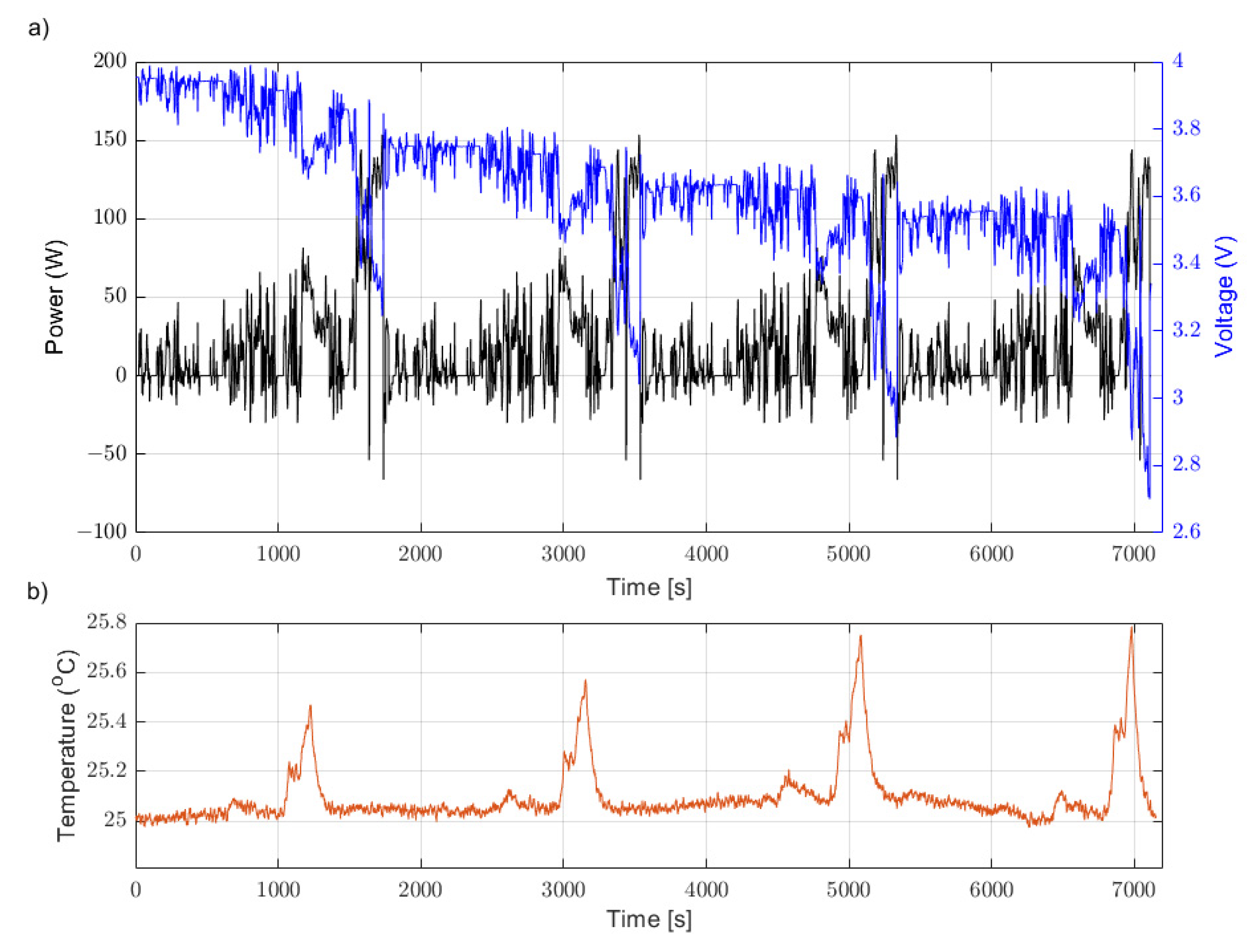
Evaluating parameter performance required a driving cycle and experimental data against which the performance of each unique parameter set could be benchmarked. The WLTP drive cycle was used as this is a common standard benchmark [
33]. This was repeated twice and scaled to create a two-hour driving cycle which would discharge exactly 60% of the cell’s quoted watt-hour capacity (
Figure 4). During the experimental process, the input to the battery cycler was a power demand time series, defining the power demanded from the cell (discharge, shown as positive in
Figure 4a) or power demanded by the cell (charge, shown as negative in
Figure 4a). The battery cycler software includes a feedback loop which reads the terminal voltage of the cell under test in order to determine the current flow out of/into the cell. This feedback loop operates at a frequency of 10 Hz. The experiments were conducted beginning at 80% SoC, thus ending approximately at 20% SoC (taking into account a slight variance given SoC is a coulombic measure and the WLTP is defined by power). This allowed the assessment of the extracted parameters across a wide SoC range. The experimental data were gathered from tests on the same cell, once again using the ICP to maintain isothermal cell surface conditions, at 25 °C and 10 °C. By way of example,
Figure 4 also shows the voltage response from the cell for the test conducted at 25 °C. It is observable in
Figure 4 that a large portion (2.72–3.97 V) of the cell’s operating window (2.7–4.2 V) was covered during the experiment. This ensured that the parameters across the full SoC of the cell were being evaluated—essential for confidence in analysis and conclusions.
The modelled results were created for each unique ECM parameter set by running the same driving cycle through the parametrised ECM. As with the experiments, the model was set to begin at 80% SoC, defined via a high resolution SoC vs. OCV dataset gathered during preliminary experiments. The model predicted cell terminal voltage as a time series over the course of the driving cycle, which was immediately comparable to the experimental data. This provided the means for a thorough investigation of the respective performance of each parameterisation experiment, as is set out in the following section.
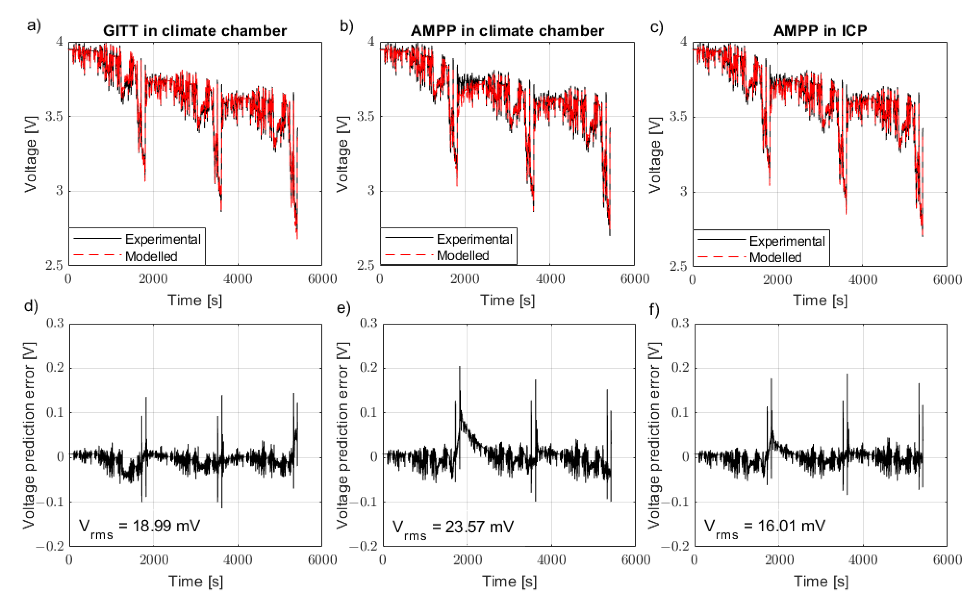
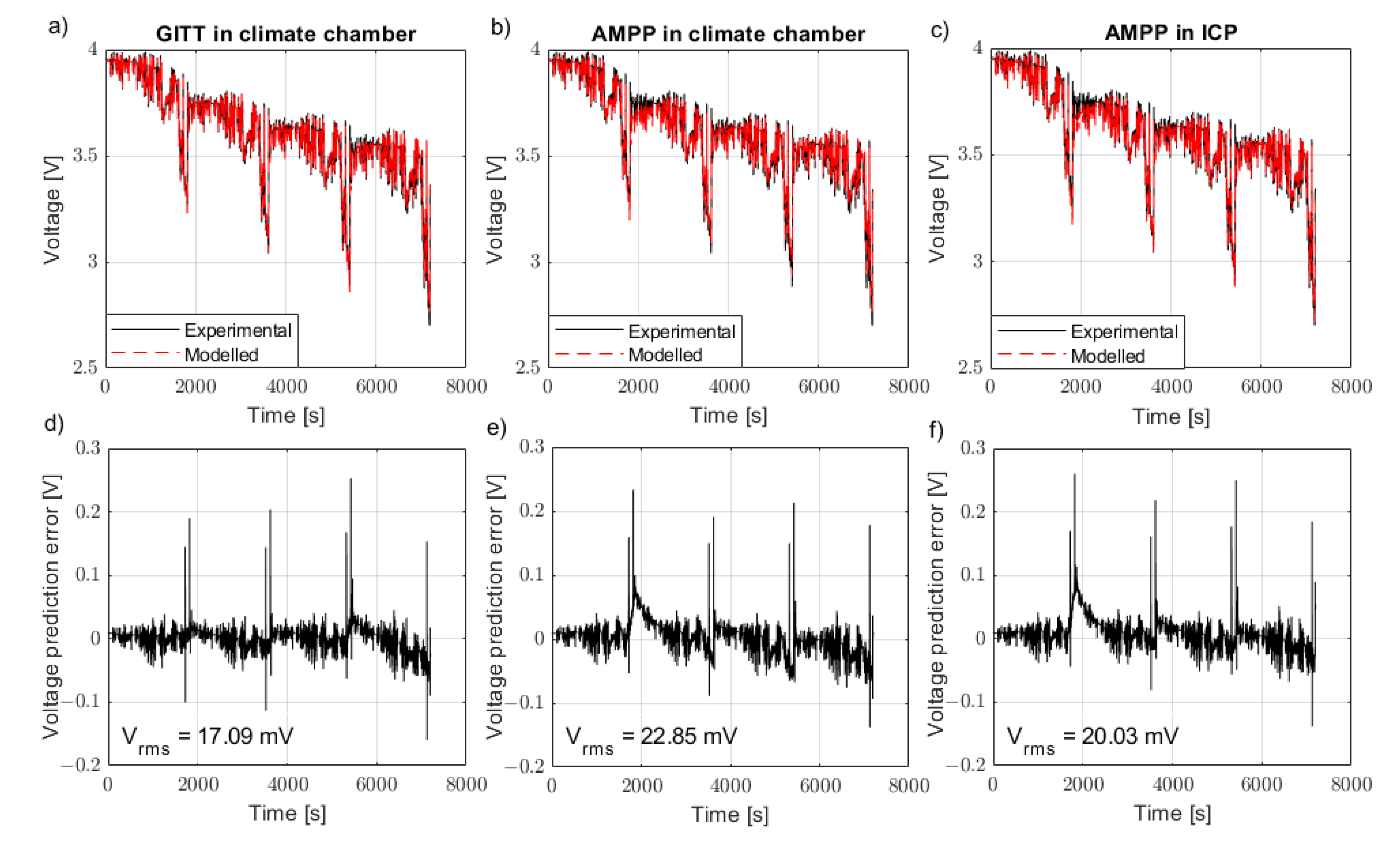
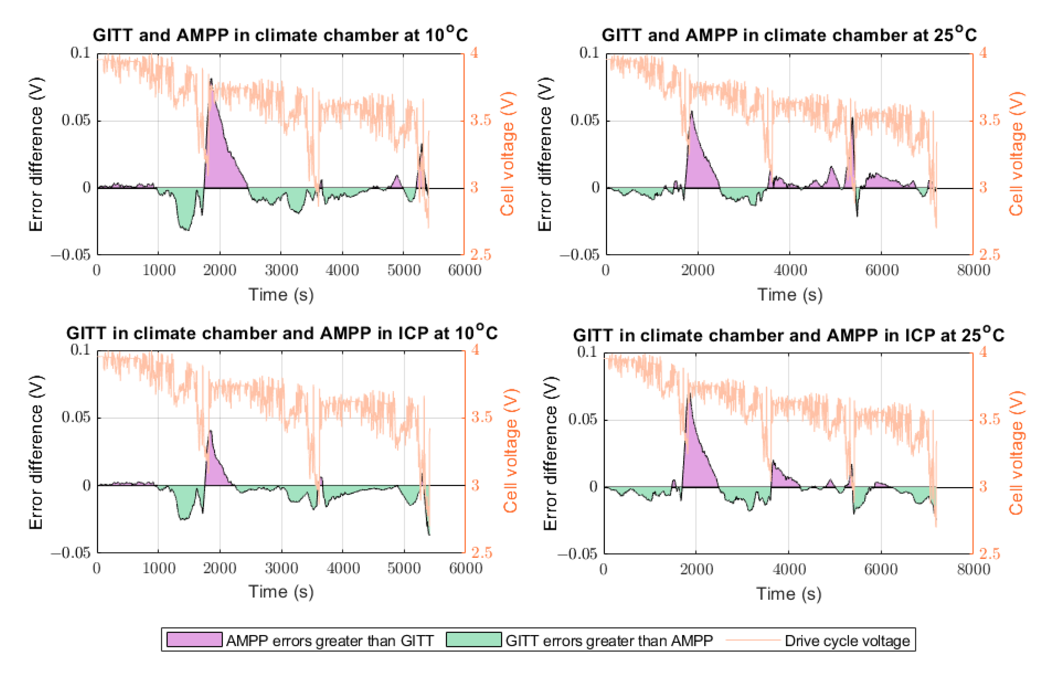
3. Drive Cycle Validation Results
A model parameterised using the AMPP technique in the climate chamber is able to carefully represent a WLTP drive cycle both at 10 °C (
Figure 5b) and 25 °C (
Figure 6b). The model parametrised using GITT, however, can better represent the model both at 10 °C (
Figure 5a) and at 25 °C in the climate chamber (
Figure 6a). By applying a superior temperature control method for the AMPP technique using the ICP, the results showed an improvement in comparison to the AMPP technique in the climate chamber. The AMPP technique in the ICP was shown to be better than that of the GITT (
Figure 5c) at 10 °C and almost as good as GITT at 25 °C (
Figure 6c). The root mean square (RMS) voltage error between the experimental drive cycle data and the predicted model emphasises the results (
Table 3). Note all modelling results are shown in
Appendix A.
4. Discussion
The AMPP technique contains a series of short duration, high C-rate pulses which induce a significant rate of heat generation. As a result, AMPP is outperformed by GITT in the climate chamber because thermal control is capped by the limitations associated with forced air convection. This reaffirms the fact that the battery industry’s current standard practice (climate chambers) for more vigorous loading cycles (such as AMPP) are not suitable when forced air convection is the means of temperature control. The presented results show that the AMPP method is enhanced with better thermal control. The AMPP data gathered from the ICP showed better agreement with GITT at 10 °C and at 25 °C compared to a climate chamber.
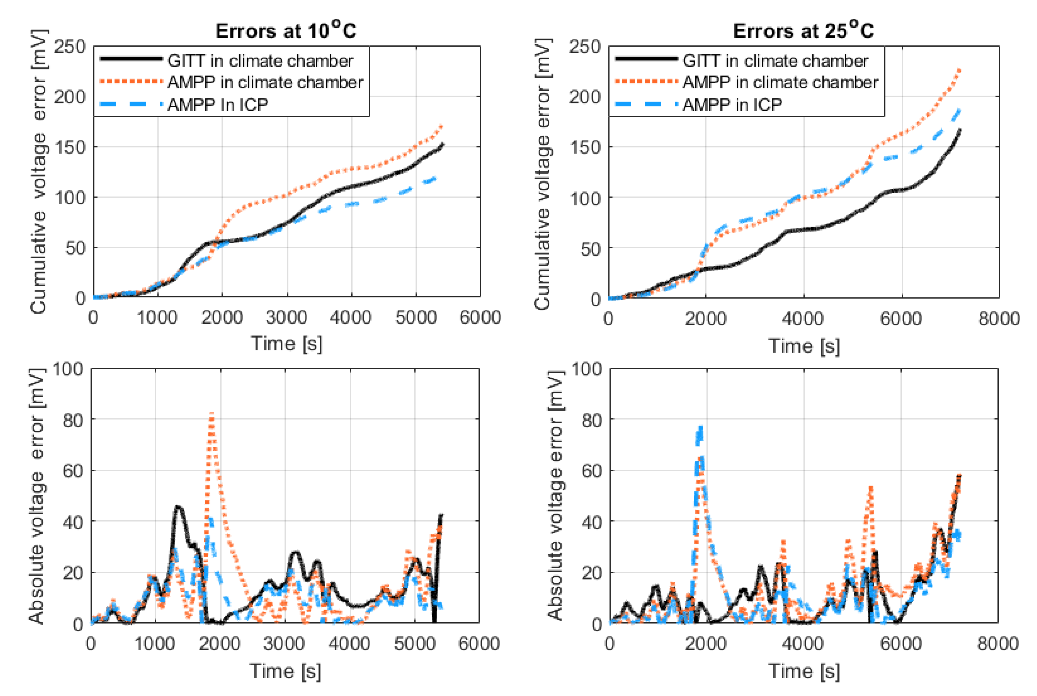
The cell produces more heat at lower temperatures due to increased cell resistance, thus errors due to temperature misrepresentation are expected to be greater at lower temperatures. This is shown in the results from this investigation: the 10 °C results have a greater cumulative error (
Figure 7) and RMS voltage error (
Table 3) for both GITT and AMPP. Note that in
Figure 7 it is important to make the comparisons of cumulative error at a given time rather than at the end of the drive cycle, because at 10 °C, the drive cycle did not complete fully, due to the lower voltage limit being reached.
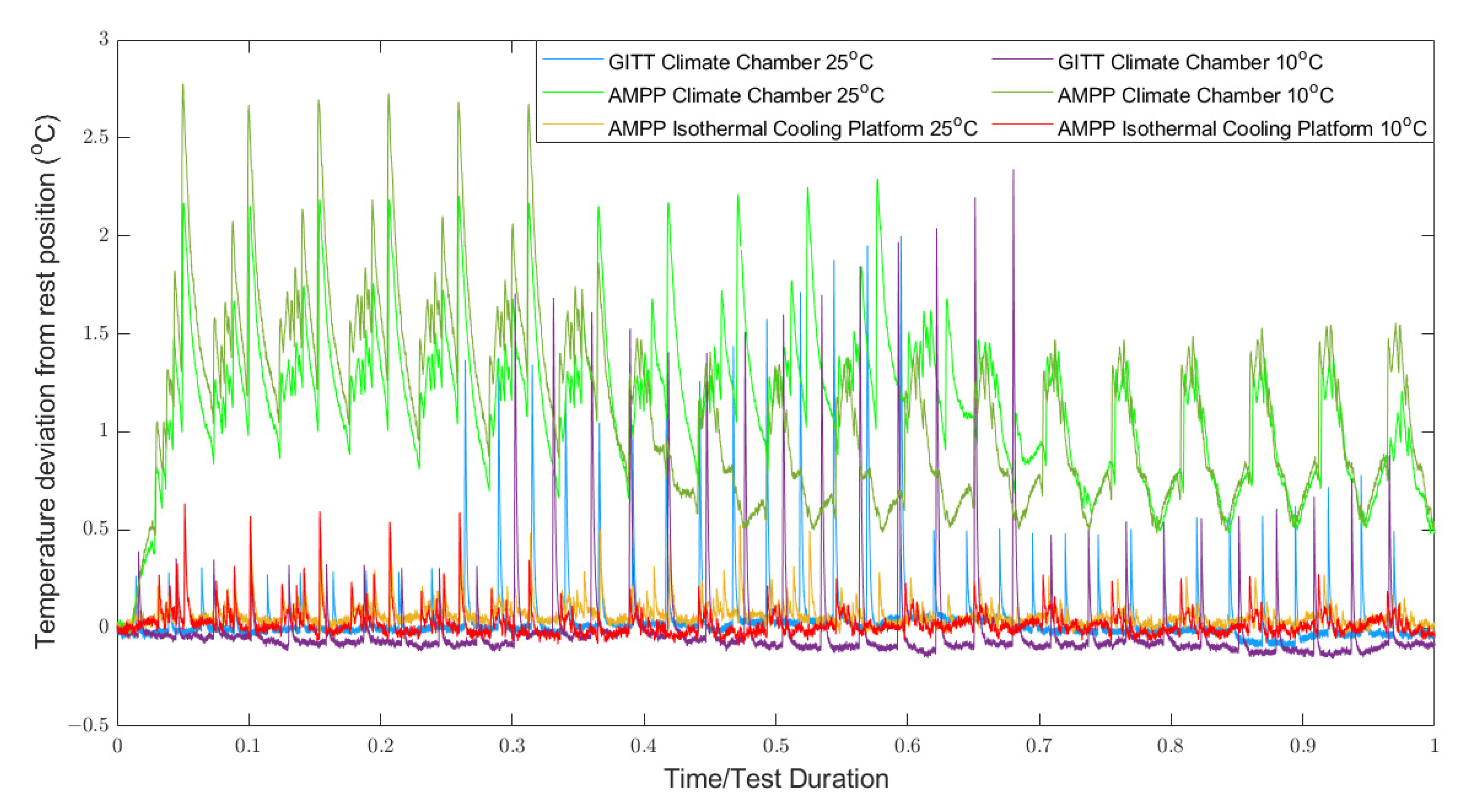
Figure 8 shows that at 10 °C, larger temperature deviations were observed in the AMPP and GITT experiments conducted in the climate chamber, compared to the AMPP experiment conducted in the ICP. The result is in line with the hypotheses—AMPP-ICP yielded the smallest RMS voltage error (
Table 3). Despite the AMPP-ICP results at 25 °C showing an improvement compared to the AMPP-climate chamber results at 25 °C, they were not found to be more accurate than the GITT-climate chamber at 25 °C (
Figure 9). This occurrence may be attributed to two factors. First, GITT at 25 °C did not produce as much heat as the data at 10°C (see
Figure 8), and, thus, the error due to temperature misrepresentation is diminished. Second, the PID control system used in the ICP was finely tuned to perform better at lower temperatures, such as 10 °C. In the data set out, the mean temperature deviation during the 10 °C ICP experiment was 0.06 °C, whilst the mean temperature deviation during the 25 °C ICP experiment was 0.09 °C. This falls into line with the outputted parameter performance—better performance from the AMPP ICP dataset recorded at 10 °C. It is difficult to quantify this correlation between temperature deviation and parameter performance with the datasets available, but this does set out a performance characteristic that could be the focus of a future investigation.
If considering the bigger picture, the difference in errors between models parametrised using AMPP and GITT are small, therefore making AMPP more beneficial than GITT mostly because it takes a shorter time to gather experimental data (AMPP is 90% faster). For example, if experimental data are required over the temperature window −20 °C to 60 °C at 5 °C intervals (which is common in industry), by using GITT, it would take 1360 h (~2 months) to gather the experimental data, whereas with AMPP it would only take 136 h (~6 days). It should be noted that the GITT used in this comparison had an SoC interval of 1% between every pulse at low and high SOCs, whereas AMPP had a 5% SoC interval for the entire SoC range. This was so that the cells’ behaviour could be captured more accurately in GITT, hence setting a higher bar in terms of model accuracy for the AMPP to be compared to. This difference in SoC intervals resulted in AMPP showing it is 90% faster than GITT. However, if the GITT test was to be repeated with a 5% SoC interval, AMPP would still be faster by 83%.
Additionally, GITT will only parametrise a model at one C-rate, whereas the C-rates in AMPP can be selected to cover multiple C-rates the cell will experience during operation. The results could be further improved by modifying AMPP such that the C-rates are closer to the application being modelled (WLTP drive cycle in this case). The AMPP technique presented here incorporated 5 C pulses whilst the WLTP drive cycle had a maximum C-rate of 1.38 C. Heat generation rate is a function of C-rate, which in turn changes the OCV of a battery. For the application of the WLTP, 5 C pulses in the parametrisation experiments cause unnecessary heating (
Figure 2) that results in the OCV drifting which ultimately results in inaccuracies in the model parameters. If the 5 C pulses in AMPP were reduced to more representative C-rates of the application being modelled, the errors would be expected to reduce.
5. Conclusions
A novel experimental technique (AMPP) for the fast parameterisation of ECMs is introduced in this paper. Its performance has been evaluated using two temperature control methods: forced air convection and conductive cooling. In all experiments, the industry standard battery model parameterisation method, GITT in a climate chamber, was used to benchmark results.
The model parametrised using GITT performed marginally better than the AMPP technique in a climate chamber. The AMPP technique contains a series of high-C-rate pulses with short rest durations and, therefore, produced significantly more heat. The AMPP technique reduced the time to complete a single experiment by more than 90% (80 h to less than 8 h)—and it must be stressed that experiments are usually performed at multiple temperatures to fully parameterise a thermally coupled ECM. This can take several weeks or even months using GITT; however, the use of AMPP reduced the testing time to a few days.
The reduction in model accuracy caused by AMPP can be compensated by employing enhanced thermal control, such as the ICP. At 25 °C, AMPP errors were reduced when the ICP was used. At 10 °C, AMPP-ICP outperformed the GITT-climate chamber. The AMPP technique could be further improved by scaling the magnitude of the pulses in AMPP to suit both a specific usage application and cells with different C-rate charging/discharging limits.
A battery model at the beginning of life will not be representative as the battery ages. Models often need to be parameterised at different stages of their life cycle and at different temperatures. GITT puts a considerable time–cost burden on the process, whereas AMPP can reduce the time–cost of this process by an order of magnitude. When coupling the AMPP technique with a conductive temperature control method such as the ICP, a set temperature can also be achieved much faster than a climate chamber. This results in saving further hours of testing time when transitioning from one temperature to the next.
The AMPP-ICP combination, therefore, offers significant benefits to the battery industry. Battery power capability and energy density will continue to rise year-on-year, and, thus, the problems associated with heat generation will intensify. We already know that convective cooling is not fit for purpose, and this provides further evidence that it is limiting the battery industry. Convective cooling forces engineers to pick parameterisation methods that do not generate too much heat or have long rest periods. Conductive cooling opens up the opportunity to use higher currents and shorter rest periods; hence, AMPP-ICP is built for the future. The ICP provides the hardware solution to manage high heat generation rates and AMPP takes advantage of this to drastically reduce the time taken to develop battery models.
Author Contributions
Conceptualization, M.A.S., A.H. and Y.P.; methodology, M.A.S. and A.H.; investigation, M.A.S.; data curation, M.A.S. and A.H.; writing—original draft preparation, M.A.S. and A.H.; writing—review and editing, M.A.S., A.H. and Y.P.; visualization, M.A.S. and A.H..; supervision, Y.P.; All authors have read and agreed to the published version of the manuscript.
Funding
This research was funded by the Innovate UK THT project (grant number 105297) and and the Faraday Institution (grant number FIIF-012).
Institutional Review Board Statement
Not applicable.
Informed Consent Statement
Not applicable.
Data Availability Statement
The data presented in this study are available on request from the corresponding author. The data are not publicly available due to confidentiality.
Acknowledgments
The authors also acknowledge the support from Thermal Hazard Technology for providing the isothermal control platform that was used in this study. The authors also thank Ruben Tomlin for the development of the code that was used for parameter extraction.
Conflicts of Interest
The authors declare no conflict of interest.
Appendix A. ECM Results
Table A1.
ECM results from GITT in a climate chamber at 10 °C.
Table A1.
ECM results from GITT in a climate chamber at 10 °C.
| SoC Fraction | OCV [V] | R0 [Ohm] | R1 [Ohm] | R2 [Ohm] | R3 [Ohm] | Tau 1 [s] | Tau 2 [s] | Tau 3 [s] |
|---|
| 0.12 | 3.4264 | 0.013214 | 0.006915 | 0.005002 | 0.011307 | 2.1 | 35 | 350 |
| 0.14 | 3.4384 | 0.013161 | 0.005421 | 0.004671 | 0.006656 | 2.1 | 35 | 350 |
| 0.16 | 3.4488 | 0.013153 | 0.003516 | 0.003635 | 0.004616 | 2.1 | 35 | 350 |
| 0.18 | 3.4593 | 0.012833 | 0.002714 | 0.002953 | 0.003563 | 2.1 | 35 | 350 |
| 0.2 | 3.4713 | 0.012638 | 0.002095 | 0.002176 | 0.00101 | 2.1 | 35 | 350 |
| 0.24 | 3.5092 | 0.012219 | 0.001611 | 0.002464 | 0.001506 | 2.1 | 35 | 350 |
| 0.28 | 3.5441 | 0.012129 | 0.001266 | 0.002048 | 0.002708 | 2.1 | 35 | 350 |
| 0.32 | 3.5715 | 0.011897 | 0.000988 | 0.002097 | 0.004851 | 2.1 | 35 | 350 |
| 0.36 | 3.5634 | 0.011758 | 0.001269 | 0.001915 | 0.017278 | 2.1 | 35 | 350 |
| 0.4 | 3.6049 | 0.011562 | 0.000966 | 0.002733 | 6.86 × 10⁻⁵ | 2.1 | 35 | 350 |
| 0.44 | 3.6187 | 0.011388 | 0.000722 | 0.002543 | 0.00461 | 2.1 | 35 | 350 |
| 0.48 | 3.6339 | 0.011293 | 0.000742 | 0.002558 | 0.003474 | 2.1 | 35 | 350 |
| 0.52 | 3.6522 | 0.011123 | 0.000864 | 0.002469 | 0.002641 | 2.1 | 35 | 350 |
| 0.56 | 3.6779 | 0.01105 | 0.000973 | 0.00216 | 0.00075 | 2.1 | 35 | 350 |
| 0.6 | 3.703 | 0.010922 | 0.001065 | 0.001823 | 0.001361 | 2.1 | 35 | 350 |
| 0.64 | 3.7406 | 0.010737 | 0.001439 | 0.001502 | 0.002944 | 2.1 | 35 | 350 |
| 0.68 | 3.7882 | 0.010662 | 0.001391 | 0.001664 | 0.001272 | 2.1 | 35 | 350 |
| 0.72 | 3.8431 | 0.009841 | 0.002736 | 0.000821 | 0.004498 | 2.1 | 35 | 350 |
| 0.76 | 3.9103 | 0.009821 | 0.002207 | 0.001229 | 2.88 × 10⁻⁷ | 2.1 | 35 | 350 |
| 0.8 | 3.9383 | 0.009786 | 0.002277 | 0.001575 | 0.009015 | 2.1 | 35 | 350 |
| 0.84 | 3.9813 | 0.009776 | 0.001953 | 0.001701 | 0.006636 | 2.1 | 35 | 350 |
| 0.9 | 4.0509 | 0.009811 | 0.002013 | 0.001416 | 0.006034 | 2.1 | 35 | 350 |
| 0.92 | 4.0754 | 0.009867 | 0.001869 | 0.001552 | 0.007399 | 2.1 | 35 | 350 |
| 0.94 | 4.0997 | 0.009873 | 0.001906 | 0.001498 | 0.007223 | 2.1 | 35 | 350 |
| 0.96 | 4.1245 | 0.009862 | 0.001972 | 0.001438 | 0.007184 | 2.1 | 35 | 350 |
Table A2.
ECM results from GITT in a climate chamber at 25 °C.
Table A2.
ECM results from GITT in a climate chamber at 25 °C.
| SoC Fraction | OCV [V] | R0 [Ohm] | R1 [Ohm] | R2 [Ohm] | R3 [Ohm] | Tau 1 [s] | Tau 2 [s] | Tau 3 [s] |
|---|
| 0.06 | 3.1947 | 0.011566 | 0.004657 | 0.003944 | 0.011147 | 2.1 | 35 | 350 |
| 0.08 | 3.3173 | 0.011566 | 0.003201 | 0.00424 | 7.80 × 10⁻⁵ | 2.1 | 35 | 350 |
| 0.1 | 3.3948 | 0.011275 | 0.002058 | 0.003386 | 5.85 × 10⁻⁵ | 2.1 | 35 | 350 |
| 0.12 | 3.4272 | 0.011096 | 0.001483 | 0.003163 | 0.005288 | 2.1 | 35 | 350 |
| 0.14 | 3.4408 | 0.010966 | 0.001202 | 0.00277 | 0.005414 | 2.1 | 35 | 350 |
| 0.16 | 3.4508 | 0.010739 | 0.001089 | 0.002444 | 0.003464 | 2.1 | 35 | 350 |
| 0.18 | 3.4612 | 0.010581 | 0.000946 | 0.002161 | 0.002244 | 2.1 | 35 | 350 |
| 0.2 | 3.4746 | 0.01046 | 0.000806 | 0.001721 | 0.001114 | 2.1 | 35 | 350 |
| 0.24 | 3.5125 | 0.01024 | 0.000658 | 0.001905 | 0.000925 | 2.1 | 35 | 350 |
| 0.28 | 3.5449 | 0.010015 | 0.000556 | 0.001934 | 0.002052 | 2.1 | 35 | 350 |
| 0.32 | 3.5723 | 0.009809 | 0.000418 | 0.002141 | 0.002555 | 2.1 | 35 | 350 |
| 0.36 | 3.5781 | 0.009725 | 0.000596 | 0.001943 | 0.010587 | 2.1 | 35 | 350 |
| 0.4 | 3.6098 | 0.009535 | 0.000423 | 0.002444 | 1.63 × 10⁻⁵ | 2.1 | 35 | 350 |
| 0.44 | 3.6234 | 0.009447 | 0.00024 | 0.002333 | 0.002955 | 2.1 | 35 | 350 |
| 0.48 | 3.6387 | 0.009276 | 0.000416 | 0.002138 | 0.00265 | 2.1 | 35 | 350 |
| 0.52 | 3.6571 | 0.009101 | 0.000611 | 0.001836 | 0.002543 | 2.1 | 35 | 350 |
| 0.56 | 3.6832 | 0.008987 | 0.000607 | 0.001724 | 0.000695 | 2.1 | 35 | 350 |
| 0.6 | 3.708 | 0.008809 | 0.000768 | 0.001234 | 0.001902 | 2.1 | 35 | 350 |
| 0.64 | 3.7458 | 0.008693 | 0.00109 | 0.000976 | 0.002376 | 2.1 | 35 | 350 |
| 0.68 | 3.797 | 0.008588 | 0.001074 | 0.001213 | 0.000836 | 2.1 | 35 | 350 |
| 0.72 | 3.8503 | 0.008484 | 0.001209 | 0.001202 | 0.003452 | 2.1 | 35 | 350 |
| 0.76 | 3.8912 | 0.008449 | 0.001347 | 0.001473 | 0.006178 | 2.1 | 35 | 350 |
| 0.8 | 3.9439 | 0.008032 | 0.001665 | 0.000752 | 3.97 × 10⁻⁸ | 2.1 | 35 | 350 |
| 0.84 | 3.9857 | 0.008013 | 0.001428 | 0.00159 | 0.002517 | 2.1 | 35 | 350 |
| 0.9 | 4.0541 | 0.008034 | 0.001364 | 0.001191 | 0.003498 | 2.1 | 35 | 350 |
| 0.92 | 4.078 | 0.008033 | 0.001124 | 0.001442 | 0.00428 | 2.1 | 35 | 350 |
| 0.94 | 4.1023 | 0.008049 | 0.001108 | 0.001411 | 0.004137 | 2.1 | 35 | 350 |
| 0.96 | 4.127 | 0.008065 | 0.001104 | 0.001379 | 0.004089 | 2.1 | 35 | 350 |
| 0.98 | 4.1542 | 0.008109 | 0.001129 | 0.001192 | 0.005278 | 2.1 | 35 | 350 |
| 1 | 4.1779 | 0.008109 | 0.001108 | 0.001246 | 0.004951 | 2.1 | 35 | 350 |
Table A3.
ECM results from AMPP in a climate chamber at 10 °C.
Table A3.
ECM results from AMPP in a climate chamber at 10 °C.
| SoC Fraction | OCV [V] | R0 [Ohm] | R1 [Ohm] | R2 [Ohm] | R3 [Ohm] | Tau 1 [s] | Tau 2 [s] | Tau 3 [s] |
|---|
| 0.24 | 3.5267 | 0.010353 | 0.00202 | 0.001369 | 0.017496 | 2.1 | 35 | 350 |
| 0.28 | 3.5521 | 0.010556 | 0.001665 | 0.001814 | 0.007756 | 2.1 | 35 | 350 |
| 0.32 | 3.5728 | 0.01051 | 0.001392 | 0.002393 | 0.005783 | 2.1 | 35 | 350 |
| 0.36 | 3.5898 | 0.010298 | 0.001402 | 0.002366 | 0.006071 | 2.1 | 35 | 350 |
| 0.4 | 3.6047 | 0.01057 | 0.000966 | 0.002492 | 0.005063 | 2.1 | 35 | 350 |
| 0.44 | 3.6195 | 0.010535 | 0.000866 | 0.002564 | 0.004764 | 2.1 | 35 | 350 |
| 0.48 | 3.6363 | 0.010581 | 0.000661 | 0.002603 | 0.004287 | 2.1 | 35 | 350 |
| 0.52 | 3.6567 | 0.010518 | 0.000695 | 0.002535 | 0.003746 | 2.1 | 35 | 350 |
| 0.56 | 3.6824 | 0.010343 | 0.000462 | 0.002931 | 0.003146 | 2.1 | 35 | 350 |
| 0.6 | 3.714 | 0.010636 | 5.17 × 10⁻⁸ | 0.002765 | 0.004001 | 2.1 | 35 | 350 |
| 0.64 | 3.7525 | 0.010506 | 4.39 × 10⁻⁸ | 0.002319 | 0.005944 | 2.1 | 35 | 350 |
| 0.68 | 3.8038 | 0.010299 | 4.66 × 10⁻¹¹ | 0.00215 | 0.00858 | 2.1 | 35 | 350 |
| 0.72 | 3.8574 | 0.010193 | 4.14 × 10⁻⁹ | 0.002427 | 0.008523 | 2.1 | 35 | 350 |
| 0.76 | 3.9024 | 0.010233 | 2.28 × 10⁻⁹ | 0.003317 | 0.006257 | 2.1 | 35 | 350 |
| 0.8 | 3.9455 | 0.010157 | 1.78 × 10⁻⁹ | 0.003096 | 0.006285 | 2.1 | 35 | 350 |
| 0.84 | 3.9892 | 0.010296 | 6.91 × 10⁻⁹ | 0.003158 | 0.00536 | 2.1 | 35 | 350 |
| 0.9 | 4.0575 | 0.010281 | 5.56 × 10⁻⁹ | 0.00233 | 0.006255 | 2.1 | 35 | 350 |
| 0.92 | 4.0809 | 0.010304 | 6.28 × 10⁻¹⁰ | 0.001559 | 0.008847 | 2.1 | 35 | 350 |
| 0.94 | 4.1044 | 0.010325 | 1.99 × 10⁻¹⁰ | 0.002053 | 0.005632 | 2.1 | 35 | 350 |
| 0.96 | 4.1284 | 0.010341 | 3.37 × 10⁻¹⁰ | 0.002397 | 0.003662 | 2.1 | 35 | 350 |
| 0.98 | 4.1532 | 0.010895 | 1.30 × 10⁻⁹ | 0.000925 | 0.005857 | 2.1 | 35 | 350 |
| 1 | 4.1834 | 0.010895 | 5.18 × 10⁻⁹ | 0.000953 | 0.005702 | 2.1 | 35 | 350 |
Table A4.
ECM results from AMPP in a climate chamber at 25 °C.
Table A4.
ECM results from AMPP in a climate chamber at 25 °C.
| SoC Fraction | OCV [V] | R0 [Ohm] | R1 [Ohm] | R2 [Ohm] | R3 [Ohm] | Tau 1 [s] | Tau 2 [s] | Tau 3 [s] |
|---|
| 0.14 | 3.4435 | 0.010587 | 0.000449 | 0.004525 | 0.000562 | 2.1 | 35 | 350 |
| 0.16 | 3.4563 | 0.010214 | 0.000897 | 0.001458 | 0.00652 | 2.1 | 35 | 350 |
| 0.18 | 3.4749 | 0.010104 | 0.000743 | 0.001471 | 0.010942 | 2.1 | 35 | 350 |
| 0.2 | 3.4939 | 0.009635 | 0.000704 | 0.002251 | 0.002036 | 2.1 | 35 | 350 |
| 0.24 | 3.5267 | 0.009341 | 0.000795 | 0.002119 | 0.002827 | 2.1 | 35 | 350 |
| 0.28 | 3.5521 | 0.009247 | 0.000738 | 0.002151 | 0.002895 | 2.1 | 35 | 350 |
| 0.32 | 3.5728 | 0.009292 | 0.000215 | 0.002444 | 0.002479 | 2.1 | 35 | 350 |
| 0.36 | 3.5898 | 0.00928 | 9.02 × 10⁻⁸ | 0.002136 | 0.002535 | 2.1 | 35 | 350 |
| 0.4 | 3.6047 | 0.009186 | 5.83 × 10⁻⁶ | 0.002124 | 0.002507 | 2.1 | 35 | 350 |
| 0.44 | 3.6195 | 0.009025 | 3.56 × 10⁻¹⁰ | 0.00185 | 0.002887 | 2.1 | 35 | 350 |
| 0.48 | 3.6363 | 0.008974 | 2.59 × 10⁻¹⁰ | 0.001601 | 0.002858 | 2.1 | 35 | 350 |
| 0.52 | 3.6567 | 0.008928 | 4.62 × 10⁻⁹ | 0.00176 | 0.002044 | 2.1 | 35 | 350 |
| 0.56 | 3.6824 | 0.008906 | 7.32 × 10⁻⁹ | 0.001844 | 0.002992 | 2.1 | 35 | 350 |
| 0.6 | 3.714 | 0.008913 | 4.54 × 10⁻⁸ | 0.001749 | 0.003692 | 2.1 | 35 | 350 |
| 0.64 | 3.7525 | 0.008805 | 1.27 × 10⁻⁹ | 0.001468 | 0.005304 | 2.1 | 35 | 350 |
| 0.68 | 3.8038 | 0.008707 | 3.94 × 10⁻¹¹ | 0.001649 | 0.006487 | 2.1 | 35 | 350 |
| 0.72 | 3.8574 | 0.00871 | 1.21 × 10⁻⁹ | 0.001916 | 0.006594 | 2.1 | 35 | 350 |
| 0.76 | 3.9024 | 0.008821 | 3.17 × 10⁻¹⁰ | 0.002154 | 0.005457 | 2.1 | 35 | 350 |
| 0.8 | 3.9455 | 0.008654 | 1.80 × 10⁻⁹ | 0.002102 | 0.005715 | 2.1 | 35 | 350 |
| 0.84 | 3.9892 | 0.008702 | 1.03 × 10⁻⁹ | 0.001831 | 0.004788 | 2.1 | 35 | 350 |
| 0.9 | 4.0575 | 0.008699 | 4.85 × 10⁻⁹ | 0.001624 | 0.003119 | 2.1 | 35 | 350 |
| 0.92 | 4.0809 | 0.008716 | 1.19 × 10⁻⁹ | 0.000969 | 0.005907 | 2.1 | 35 | 350 |
| 0.94 | 4.1044 | 0.008727 | 8.10 × 10⁻¹⁰ | 0.00094 | 0.004866 | 2.1 | 35 | 350 |
| 0.96 | 4.1284 | 0.008799 | 1.58 × 10⁻⁹ | 0.001428 | 0.003859 | 2.1 | 35 | 350 |
| 0.98 | 4.1532 | 0.009068 | 4.23 × 10⁻⁸ | 3.58 × 10⁻⁵ | 0.004334 | 2.1 | 35 | 350 |
| 1 | 4.1834 | 0.009068 | 3.37 × 10⁻⁸ | 7.36 × 10⁻⁵ | 0.004213 | 2.1 | 35 | 350 |
Table A5.
ECM results from AMPP in the ICP at 10 °C.
Table A5.
ECM results from AMPP in the ICP at 10 °C.
| SoC Fraction | OCV [V] | R0 [Ohm] | R1 [Ohm] | R2 [Ohm] | R3 [Ohm] | Tau 1 [s] | Tau 2 [s] | Tau 3 [s] |
|---|
| 0.28 | 3.5789 | 0.012479 | 5.90 × 10⁻⁵ | 0.001911 | 0.017716 | 2.1 | 35 | 350 |
| 0.32 | 3.5972 | 0.012398 | 7.84 × 10⁻⁹ | 0.002045 | 0.007293 | 2.1 | 35 | 350 |
| 0.36 | 3.6121 | 0.011859 | 0.000337 | 0.002049 | 0.006787 | 2.1 | 35 | 350 |
| 0.4 | 3.6261 | 0.011751 | 0.000166 | 0.00203 | 0.005824 | 2.1 | 35 | 350 |
| 0.44 | 3.6406 | 0.011522 | 0.000306 | 0.002134 | 0.00633 | 2.1 | 35 | 350 |
| 0.48 | 3.6573 | 0.011426 | 0.000176 | 0.002168 | 0.004879 | 2.1 | 35 | 350 |
| 0.52 | 3.678 | 0.011388 | 7.98 × 10⁻⁵ | 0.002295 | 0.004387 | 2.1 | 35 | 350 |
| 0.56 | 3.7042 | 0.011158 | 0.000197 | 0.00233 | 0.003584 | 2.1 | 35 | 350 |
| 0.6 | 3.7367 | 0.011256 | 6.43 × 10⁻⁶ | 0.002313 | 0.003845 | 2.1 | 35 | 350 |
| 0.64 | 3.7758 | 0.010951 | 0.00027 | 0.00238 | 0.001264 | 2.1 | 35 | 350 |
| 0.68 | 3.8272 | 0.010795 | 0.000386 | 0.002429 | 0.000828 | 2.1 | 35 | 350 |
| 0.72 | 3.8784 | 0.010997 | 9.10 × 10⁻⁵ | 0.00272 | 0.003992 | 2.1 | 35 | 350 |
| 0.76 | 3.9211 | 0.010774 | 0.000356 | 0.002739 | 0.003176 | 2.1 | 35 | 350 |
| 0.8 | 3.9629 | 0.010782 | 0.000419 | 0.002656 | 0.005652 | 2.1 | 35 | 350 |
| 0.84 | 4.0061 | 0.010869 | 0.000314 | 0.003693 | 0.004532 | 2.1 | 35 | 350 |
| 0.9 | 4.0736 | 0.010869 | 0.000324 | 0.003642 | 0.005104 | 2.1 | 35 | 350 |
| 0.92 | 4.0966 | 0.010869 | 0.000491 | 0.009964 | 0.022232 | 2.1 | 35 | 350 |
| 0.94 | 4.1199 | 0.010095 | 0.001508 | 0.002207 | 0.000808 | 2.1 | 35 | 350 |
| 0.96 | 4.1434 | 0.010326 | 0.001334 | 0.001932 | 0.004348 | 2.1 | 35 | 350 |
| 0.98 | 4.1675 | 0.012926 | 0.000922 | 0.006324 | 0.045332 | 2.1 | 35 | 350 |
| 1 | 4.1917 | 0.012926 | 0.001576 | 0.002926 | 0.14491 | 2.1 | 35 | 350 |
Table A6.
ECM results from AMPP in the ICP at 25 °C.
Table A6.
ECM results from AMPP in the ICP at 25 °C.
| SoC Fraction | OCV [V] | R0 [Ohm] | R1 [Ohm] | R2 [Ohm] | R3 [Ohm] | Tau 1 [s] | Tau 2 [s] | Tau 3 [s] |
|---|
| 0.16 | 3.482 | 0.010987 | 0.000156 | 0.001118 | 0.0423 | 2.1 | 35 | 350 |
| 0.18 | 3.5007 | 0.010877 | 0.000249 | 0.001396 | 0.018332 | 2.1 | 35 | 350 |
| 0.2 | 3.5194 | 0.010521 | 0.000266 | 0.001841 | 0.002775 | 2.1 | 35 | 350 |
| 0.24 | 3.5521 | 0.010118 | 0.000462 | 0.001764 | 0.002666 | 2.1 | 35 | 350 |
| 0.28 | 3.5789 | 0.010012 | 0.000227 | 0.001816 | 0.003232 | 2.1 | 35 | 350 |
| 0.32 | 3.5972 | 0.009914 | 0.000212 | 0.001791 | 0.00469 | 2.1 | 35 | 350 |
| 0.36 | 3.6121 | 0.009721 | 0.000204 | 0.00158 | 0.003682 | 2.1 | 35 | 350 |
| 0.4 | 3.6261 | 0.009471 | 0.000303 | 0.001988 | 0.002044 | 2.1 | 35 | 350 |
| 0.44 | 3.6406 | 0.009259 | 0.000474 | 0.001869 | 0.000774 | 2.1 | 35 | 350 |
| 0.48 | 3.6573 | 0.009369 | 0.000216 | 0.001848 | 0.001556 | 2.1 | 35 | 350 |
| 0.52 | 3.678 | 0.009 | 0.000483 | 0.001893 | 0.001984 | 2.1 | 35 | 350 |
| 0.56 | 3.7042 | 0.009129 | 0.000196 | 0.002019 | 0.001945 | 2.1 | 35 | 350 |
| 0.6 | 3.7367 | 0.008922 | 0.000302 | 0.002095 | 0.001247 | 2.1 | 35 | 350 |
| 0.64 | 3.7758 | 0.008797 | 0.000444 | 0.001828 | 0.001518 | 2.1 | 35 | 350 |
| 0.68 | 3.8272 | 0.008883 | 0.000271 | 0.001997 | 0.004159 | 2.1 | 35 | 350 |
| 0.72 | 3.8784 | 0.008656 | 0.000487 | 0.002161 | 0.001445 | 2.1 | 35 | 350 |
| 0.76 | 3.9211 | 0.008793 | 0.000354 | 0.002173 | 0.004858 | 2.1 | 35 | 350 |
| 0.8 | 3.9629 | 0.008568 | 0.000683 | 0.001989 | 0.002537 | 2.1 | 35 | 350 |
| 0.84 | 4.0061 | 0.008569 | 0.000545 | 0.002071 | 0.003489 | 2.1 | 35 | 350 |
| 0.9 | 4.0736 | 0.008569 | 0.000496 | 0.002331 | 0.002812 | 2.1 | 35 | 350 |
| 0.92 | 4.0966 | 0.008546 | 0.000441 | 0.001331 | 0.005019 | 2.1 | 35 | 350 |
| 0.94 | 4.1199 | 0.008399 | 0.000664 | 0.001863 | 0.001328 | 2.1 | 35 | 350 |
| 0.96 | 4.1434 | 0.008564 | 0.000479 | 0.00197 | 0.00155 | 2.1 | 35 | 350 |
| 0.98 | 4.1675 | 0.009163 | 3.02 × 10⁻⁷ | 0.00164 | 0.004176 | 2.1 | 35 | 350 |
| 1 | 4.1917 | 0.009163 | 5.79 × 10⁻⁶ | 0.001796 | 0.002301 | 2.1 | 35 | 350 |
References
- Shi, H.; Wang, S.; Fernandez, C.; Yu, C.; Xu, W.; Dablu, B.E.; Wang, L. Improved multi-time scale lumped thermoelectric coupling modeling and parameter dispersion evaluation of lithium-ion batteries. Appl. Energy 2022, 324, 119789. [Google Scholar] [CrossRef]
- Wu, L.; Liu, K.; Pang, H. Evaluation and observability analysis of an improved reduced-order electrochemical model for lithium-ion battery. Electrochim. Acta 2021, 368, 137604. [Google Scholar] [CrossRef]
- Meng, J.; Luo, G.; Ricco, M.; Swierczynski, M.; Stroe, D.-I.; Teodorescu, R. Overview of Lithium-Ion Battery Modeling Methods for State-of-Charge Estimation in Electrical Vehicles. Appl. Sci. 2018, 8, 659. [Google Scholar] [CrossRef]
- Barai, A.; Ashwin, T.R.; Iraklis, C.; McGordon, A.; Jennings, P. Scale-up of lithium-ion battery model parameters from cell level to module level—Identification of current issues. Energy Procedia 2017, 138, 223–228. [Google Scholar] [CrossRef]
- Taylor, J.; Barai, A.; Ashwin, T.R.; Guo, Y.; Amor-Segan, M.; Marco, J. An insight into the errors and uncertainty of the lithium-ion battery characterisation experiments. J. Energy Storage 2019, 24, 100761. [Google Scholar] [CrossRef]
- Do, D.V.; Forgez, C.; El Kadri Benkara, K.; Friedrich, G. Impedance observer for a Li-ion battery using Kalman filter. IEEE Trans. Veh. Technol. 2009, 58, 3930–3937. [Google Scholar]
- Andre, D.; Meiler, M.; Steiner, K.; Walz, H.; Soczka-Guth, T.; Sauer, D.U. Characterization of high-power lithium-ion batteries by electrochemical impedance spectroscopy. II: Modelling. J. Power Sources 2011, 196, 5349–5356. [Google Scholar] [CrossRef]
- Ecker, M.; Tran, T.K.D.; Dechent, P.; Käbitz, S.; Warnecke, A.; Sauer, D.U. Parameterization of a Physico-Chemical Model of a Lithium-Ion Battery: I. Determination of Parameters. J. Electrochem. Soc. 2015, 162, A1836. [Google Scholar] [CrossRef]
- Hsieh, Y.-C.; Lin, T.-D.; Chen, R.-J.; Lin, H.-Y. Electric circuit modelling for lithium-ion batteries by intermittent discharging. IET Power Electron. 2014, 7, 2672–2677. [Google Scholar] [CrossRef]
- Hentunen, A.; Lehmuspelto, T.; Suomela, J. Time-domain parameter extraction method for thévenin-equivalent circuit battery models. IEEE Trans. Energy Convers. 2014, 29, 558–566. [Google Scholar] [CrossRef]
- Zhao, Y.; Patel, Y.; Zhang, T.; Offer, G.J. Modeling the Effects of Thermal Gradients Induced by Tab and Surface Cooling on Lithium Ion Cell Performance. J. Electrochem. Soc. 2018, 165, A3169–A3178. [Google Scholar] [CrossRef]
- Li, S.; Kirkaldy, N.; Zhang, C.; Gopalakrishnan, K.; Amietszajew, T.; Diaz, L.B.; Barreras, J.V.; Shams, M.; Hua, X.; Patel, Y.; et al. Optimal cell tab design and cooling strategy for cylindrical lithium-ion batteries. J. Power Sources 2021, 492, 229594. [Google Scholar] [CrossRef]
- Hales, A.; Brouillet, E.; Wang, Z.; Edwards, B.; Samieian, M.A.; Kay, J.; Mores, S.; Auger, D.; Patel, Y.; Offer, G. Isothermal Temperature Control for Battery Testing and Battery Model Parameterization. SAE Int. J. Electrified Veh. 2021, 10, 105–122. [Google Scholar] [CrossRef]
- Li, J.; Mazzola, M.; Gafford, J.; Younan, N. A new parameter estimation algorithm for an electrical analogue battery model. In Proceedings of the 2012 Twenty-Seventh Annual IEEE Applied Power Electronics Conference and Exposition (APEC), Orlando, FL, USA, 5–9 February 2012; pp. 427–433. [Google Scholar]
- Zheng, Y.; Shi, Z.; Guo, D.; Dai, H.; Han, X. A simplification of the time-domain equivalent circuit model for lithium-ion batteries based on low-frequency electrochemical impedance spectra. J. Power Sources 2021, 489, 229505. [Google Scholar] [CrossRef]
- Li, Z.; Shi, X.; Shi, M.; Wei, C.; Di, F.; Sun, H. Investigation on the Impact of the HPPC Profile on the Battery ECM Parameters’ Offline Identification. In Proceedings of the 2020 Asia Energy and Electrical Engineering Symposium (AEEES), Chengdu, China, 29–31 May 2020; pp. 753–757. [Google Scholar]
- Tran, M.K.; Mevawala, A.; Panchal, S.; Raahemifar, K.; Fowler, M.; Fraser, R. Effect of integrating the hysteresis component to the equivalent circuit model of Lithium-ion battery for dynamic and non-dynamic applications. J. Energy Storage 2020, 32, 101785. [Google Scholar] [CrossRef]
- Khan, K.; Jafari, M.; Gauchia, L. Comparison of Li-ion battery equivalent circuit modelling using impedance analyzer and Bayesian networks. IET Electr. Syst. Transp. 2018, 8, 197–204. [Google Scholar] [CrossRef]
- Weppner, W.; Huggins, R.A. Determination of the Kinetic Parameters of Mixed-Conducting Electrodes and Application to the System Li3Sb. J. Electrochem. Soc. 1977, 124, 1569. [Google Scholar] [CrossRef]
- Stockley, T.; Thanapalan, K.; Bowkett, M.; Williams, J. Development of an OCV prediction mechanism for lithium-ion battery system. In Proceedings of the 2013 19th International Conference on Automation and Computing, London, UK, 13–14 July 2013; pp. 1–6. [Google Scholar]
- Li, A.; Pelissier, S.; Venet, P.; Gyan, P. Fast characterization method for modeling battery relaxation voltage. J. Batter Technol. Mater. 2016, 2, 7. [Google Scholar] [CrossRef]
- Ecker, M.; Käbitz, S.; Laresgoiti, I.; Sauer, D.U. Parameterization of a Physico-Chemical Model of a Lithium-Ion Battery: II. Model Validation. J. Electrochem. Soc. 2015, 162, A1849. [Google Scholar] [CrossRef]
- Jackey, R.; Saginaw, M.; Sanghvi, P.; Gazzarri, J.; Huria, T.; Ceraolo, M. Battery model parameter estimation using a layered technique: An example using a lithium iron phosphate cell. SAE Tech. Pap. 2013, 2. [Google Scholar] [CrossRef]
- Rafik, F.; Gualous, H.; Gallay, R.; Crausaz, A.; Berthon, A. Frequency, thermal and voltage supercapacitor characterization and modeling. J. Power Sources 2007, 165, 928–934. [Google Scholar] [CrossRef]
- Srinivasan, V.; Wang, C.Y. Analysis of Electrochemical and Thermal Behavior of Li-Ion Cells. J. Electrochem. Soc. 2003, 150, A98. [Google Scholar] [CrossRef]
- Zhang, C.; Allafi, W.; Dinh, Q.; Ascencio, P.; Marco, J. Online estimation of battery equivalent circuit model parameters and state of charge using decoupled least squares technique. Energy 2018, 142, 678–688. [Google Scholar] [CrossRef]
- Allafi, W.; Zhang, C.; Uddin, K.; Worwood, D.; Dinh, T.Q.; Ormeno, P.A.; Li, K.; Marco, J. A lumped thermal model of lithium-ion battery cells considering radiative heat transfer. Appl. Therm. Eng. 2018, 143, 472–481. [Google Scholar] [CrossRef]
- Waldmann, T.; Bisle, G.; Hogg, B.-I.; Stumpp, S.; Danzer, M.A.; Kasper, M.; Axmann, P.; Wohlfahrt-Mehrens, M. Influence of Cell Design on Temperatures and Temperature Gradients in Lithium-Ion Cells: An In Operando Study. J. Electrochem. Soc. 2015, 162, A921–A927. [Google Scholar] [CrossRef]
- Eiland, R.; Edward Fernandes, J.; Vallejo, M.; Siddarth, A.; Agonafer, D.; Mulay, V. Thermal Performance and Efficiency of a Mineral Oil Immersed Server Over Varied Environmental Operating Conditions. J. Electron. Packag. 2017, 139, 041005. [Google Scholar]
- Trimbake, A.; Singh, C.P.; Krishnan, S. Mineral Oil Immersion Cooling of Lithium-Ion Batteries: An Experimental Investigation. J. Electrochem. Energy Convers. Storage 2022, 19, 021007. [Google Scholar]
- Chen, D.; Jiang, J.; Kim, G.H.; Yang, C.; Pesaran, A. Comparison of different cooling methods for lithium ion battery cells. Appl. Therm. Eng. 2016, 94, 846–854. [Google Scholar] [CrossRef]
- Ardani, M.I.; Patel, Y.; Siddiq, A.; Offer, G.J.; Martinez-Botas, R.F. Combined experimental and numerical evaluation of the differences between convective and conductive thermal control on the performance of a lithium ion cell. Energy 2018, 144, 81–97. [Google Scholar] [CrossRef]
- WLTP Drive Cycle [Internet]. European Automobile Manufacturers Association. 2017. Available online: https://www.wltpfacts.eu/wp-content/uploads/2017/04/WLTP_Leaflet_FA_web.pdf (accessed on 10 July 2022).
Figure 1.
Schematic of a third-order equivalent circuit.
Figure 1.
Schematic of a third-order equivalent circuit.
Figure 2.
(a) GITT profile applied across the full voltage window of the cell (4.2–2.7 V) (b) AMPP profile applied across the entire voltage window of the cell, 4.2–2.7 V. (c) Detailed view of the Current and Temperature profile of the AMPP technique from the segment show in the red box of (b).
Figure 2.
(a) GITT profile applied across the full voltage window of the cell (4.2–2.7 V) (b) AMPP profile applied across the entire voltage window of the cell, 4.2–2.7 V. (c) Detailed view of the Current and Temperature profile of the AMPP technique from the segment show in the red box of (b).
Figure 3.
Isothermal control platform (ICP) using Peltier elements to control cell temperature with conductive heat transfer through metallic blocks.
Figure 3.
Isothermal control platform (ICP) using Peltier elements to control cell temperature with conductive heat transfer through metallic blocks.
Figure 4.
WLTP drive cycle, repeated twice, used to evaluate performance of each set of extracted ECM parameters at 25 °C in the ICP. (a) Power and Voltage data; (b) Temperature data.
Figure 4.
WLTP drive cycle, repeated twice, used to evaluate performance of each set of extracted ECM parameters at 25 °C in the ICP. (a) Power and Voltage data; (b) Temperature data.
Figure 5.
Drive cycle validation along with associated error for the model parametrised using the GITT data in the climate chamber, AMPP data in the climate chamber and AMPP data in the ICP at 10 °C. The comparison of the ECM to experimental drive cycle data is shown in subfigures (a–c), whilst their associated error is shown in subfigures (d–f).
Figure 6.
Drive cycle validation along with associated error for the model parameterised using the GITT data in the climate chamber, AMPP data in the climate chamber and AMPP data in the ICP at 25 °C. The comparison of the ECM to experimental drive cycle data is shown in subfigures (a–c), whilst their associated error is shown in subfigures (d–f).
Figure 7.
Comparison of error between the experimental data and the model parameterised using different experimental techniques at 10 °C and 25 °C. The cumulative absolute voltage error (top) and the absolute voltage error (bottom). To ease the visualisation of the major trends in the graph, a moving average with a window size of 200 and sampling rate of 2 Hz was applied.
Figure 8.
Temperature deviation from the rest position during the experiments used for parametrisation. Temperature was measured using type-K thermocouples.
Figure 8.
Temperature deviation from the rest position during the experiments used for parametrisation. Temperature was measured using type-K thermocouples.
Figure 9.
Difference in error between the ECM models parametrised using the different techniques against the WLTP drive cycle. The purple colour represents the region where the ECM produced from the AMPP data showed greater error than the ECM produced from the GITT data. The green colour represents the region where the ECM produced from the GITT data showed greater error than the ECM produced from the AMPP data.
Table 1.
Specification of pouch cell used in the experiments.
Table 1.
Specification of pouch cell used in the experiments.
| Capacity | Imax Charge | Imax Discharge | Imax Pulse Discharge | Vmax | Vmin |
|---|
| 20 Ah | 20 A | 70 A | 100 A | 4.2 V | 2.7 V |
Table 2.
Step specification of the AMPP technique.
Table 2.
Step specification of the AMPP technique.
| Procedure | Duration (s) |
|---|
| Discharge −0.5 C | 360 |
| Rest | 60 |
| Discharge −3 C | 10 |
| Rest | 60 |
| Charge 1 C | 77 |
| Rest | 60 |
| Discharge −3 C | 5 |
| Rest | 60 |
| Discharge −5 C | 3 |
| Rest | 60 |
| Discharge −3 C | 3 |
| Rest | 60 |
| Discharge −5 C | 5 |
| Rest | 60 |
| Charge 0.5 C | 154 |
| Rest | 60 |
| Discharge −5 C | 10 |
| Rest | 60 |
| Discharge −1 C | 10 |
| Rest | 60 |
Table 3.
Voltage RMS error in the model relative to the drive cycle experimental data.
Table 3.
Voltage RMS error in the model relative to the drive cycle experimental data.
| Temperature (°C) | ECM Parameterised Using GITT in Climate Chamber
(mV) | ECM Parameterised Using AMPP in Climate Chamber
(mV) | ECM Parameterised Using AMPP in ICP
(mV) |
|---|
| 25 | 17.09 | 22.85 | 20.03 |
| 10 | 18.99 | 23.57 | 16.01 |
| Publisher’s Note: MDPI stays neutral with regard to jurisdictional claims in published maps and institutional affiliations. |
© 2022 by the authors. Licensee MDPI, Basel, Switzerland. This article is an open access article distributed under the terms and conditions of the Creative Commons Attribution (CC BY) license (https://creativecommons.org/licenses/by/4.0/).


