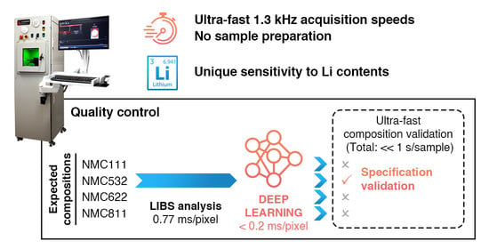
Deep Learning Classification of Li-Ion Battery Materials Targeting Accurate Composition Classification from Laser-Induced Breakdown Spectroscopy High-Speed Analyses

Abstract

Laser-induced breakdown spectroscopy (LIBS) is a valuable tool for the solid-state elemental analysis of battery materials. Key advantages include a high sensitivity for light elements (lithium included), complex emission patterns unique to individual elements through the full periodic table, and record speed analysis reaching 1300 full spectra per second (1.3 kHz acquisition rate). This study investigates deep learning methods as an alternative tool to accurately recognize different compositions of similar battery materials regardless of their physical properties or manufacturer. Such applications are of interest for the real-time digitalization of battery components and identification in automated manufacturing and recycling plant designs.

1. Introduction

Rechargeable batteries are pivotal to grid-scale applications and greener transportation systems [1]. With the exponential growth of the battery industry, battery material producers are facing an ever-increasing demand for high-technology materials. Furthermore, raw materials entering production processes and supplied active materials need to stringent quality control. Quality control is a mandatory, albeit time-consuming, operation and requires time-efficient analytical methods.

Along with manufacturing concerns, Li-ion batteries should be integrated into a circular economy where recycling the different components must be done in a safe and efficient way. The variety of battery chemistries with numerous kinds of active materials can burden both manufacturing and recycling processes with several separation and purification steps. The qualification of battery chemistries prior to the shredding process or analysis of the black mass thus relies on using a fast and reliable analytical tool. Instruments and techniques used for composition validation are not all applicable to automated processes, especially when such instruments cannot reach real-time sensing, a crucial parameter in automation [2,3].

For example, X-ray diffraction (XRD) is a useful instrument to obtain structural/microstructural information and is often used to assess the purity of crystalline materials. XRD is a crucial instrument for the synthesis and quality control of Li-ion battery components and during cycling. Although XRD is crucial for quantitative failure analysis, the need to gather data on elemental contents to diagnose impurities and direct Li contents, even in amorphous materials, is crucial. Other techniques, such as X-ray photoelectron spectroscopy (XPS) or scanning electron microscope–energy dispersive spectroscopy (SEM-EDS), are key tools for battery research, but require long analysis times and special experimental conditions. Methods used for content validation such as induced-coupled plasma methods are high-maintenance; they require gas vectors, long digestion of samples, and special clean laboratory conditions, and they do not provide any spatial information. Furthermore, tubing needs to be changed regularly and parts such as the plasma torch need to be cleaned, in aqua regia, for instance, for hours. Overall, available technologies lack sensitivity to lithium contents, are high-maintenance, and/or require long analysis times; thus, they do not generate a massive amount of information at reasonable speeds.

A more versatile elemental content analyzer with low analysis speeds could be complementary to such analysis for better diagnosis. Recent advances in the manufacturing of laser-induced breakdown spectroscopy (LIBS) instruments have brought this technology to the frontier of high-throughput data gathering. For example, we recently reported LIBS mappings at speeds reaching 1 ms per pixel [4,5]. This technology is based on atomic emission spectroscopy, which means multiple transition energies can be detected per element, making this technique highly specific. All elements can be detected, and light elements exhibit a particularly sensitive LIBS signal down to mid ppb. For example, lithium has been quantified using a high-throughput ELEMISSION instrument, with high accuracy in spodumene minerals, which are raw material for Li-ion battery materials manufacturing [6]. Despite being a promising analytical technique, very few studies of LIBS applied to energy storage applications have been reported in the literature. For research applications, LIBS has been mainly applied for lithium quantification of (Cr, Mo) doped-Li(Ni_1-x-yMn_xCo_y)O₂ (NMC) [7], LiCoO₂ (LCO) [8], micro-structures at laminated positive electrodes [9,10,11,12], and graphite negative electrodes [13,14,15]. Lithium contents in solid-state electrolyte interphases have also been studied by Hou et al. using a femtosecond LIBS instrument at a reported 0.7 µm depth resolution [16]. For process applications, LIBS has been studied for heavy metal contents in Zn-Mn batteries [17] and Pb contents in polypropylene from car battery solid wastes [18].

A very powerful advantage of using LIBS instruments is that individual emission spectra are very complex and specific, such as fingerprints of the elemental makeup of the analyzed samples. However, due to the ruggedness of samples and high sensitivity to even trace amounts of certain elements, the question of whether LIBS analysis can be used to differentiate similar compositions of pure battery materials arises. A study of the practical sensitivity of the LIBS technology must be performed on a range of battery materials to test whether this technique can be applied to analyses of composition and trace elements contents for recycling digitalization, as well as manufacturing quality assurance and quality control. For composition studies, artificial intelligence algorithms can be put to the test to improve accuracy results, speed up the compositional study, and extend applications of the LIBS technology to any target, regardless of changes in analytical parameters.

Each element exhibits unique atomic emission patterns, and these patterns are ideal inputs to artificial intelligence algorithms. Algorithms such as the angle mapper (AM) [19], support vector machine (SVM) [20,21], and random forest (RF) [22] have been used to accurately automate the identification of different mineral phases. Despite exhibiting interesting results, shallow machine learning algorithms do not allow a high control of the bias because only a few hyperparameters are typically required. Overall, poor control on underfitting and overfitting arises, especially when working with highly complex LIBS spectra. A typical issue is that spectra can be assigned to the wrong class due to fitting the model on background noises or signals from impurities.

A solution is to use artificial neural networks, or even deep learning architecture to solve classification issues in LIBS spectra of similar composition materials.

Algorithms such as artificial neural networks (ANN) show promising capabilities in the literature when applied to mineral [23] and iron ore [24] classification. The number of activation units is a controllable hyperparameter that provides certain control of the fitting function. A further step is to increase the number of layers of activation function between the input and output layers. Methods that use deep artificial neural networks are also referred to as deep learning. Ultimate control of the bias is provided by deep learning, as many hyperparameters can be tuned to manage an accurate fitting function. For example, increasing the number of units per layer or number of layers, adding a bottleneck architecture, varying the type of activation functions, etc. all allow better fitting of the trained function. A particular example of deep neural network architectures is the convolutional neural network (CNN), where different parts of the inputs to a convolutional layer are processed in the same way through shared weights. To date, there has been no investigation of the impact of the above parameters on LIBS spectra classification. As a general tendency, researchers typically jump into deep learning by providing a complex successful CNN architecture without reporting the performance of a simpler and faster architecture. As a matter of fact, papers on classification pairing LIBS and deep learning seldom report a simpler architecture than CNN and rarely report overfitting studies. In the same way, successful mineral classifications have been reported using a CNN architecture [25,26,27,28,29]. To apply this to synthetic materials such as battery materials, a more thorough study is needed, as pure contents are available, which means simpler deep learning architecture with similar accuracies could be used instead of CNN to speed up processing times.

Most of the literature on the classification of LIBS spectra has been reported on alloys or minerals. Natural mineral phases bear impurities, textures, and grain sizes that are different than synthetic inorganic materials. Furthermore, the low variation of LIBS spectra in battery material phases at different states of lithiation is expected to be much harder to classify with high accuracy than natural materials. The high purity of battery materials and small variations in different compositions provides a unique opportunity to study underfitting and overfitting in controlled samples using deep learning algorithms. The aim of this work is to compare the performance of different machine learning algorithms and deep learning architectures for the classification of different battery materials, and more importantly for the industry, to classify different compositions of the same battery material. For example, different phases of NMC (namely LiNi_1-x-yMn_xCo_yO_2, where x and y are respectively 0.33 and 0.33 (NMC111); 0.3 and 0.2 (NMC532); 0.2 and 0.2 (NMC622); and 0.1 and 0.1 (NMC811)) are commercially available and expected to exhibit very little Ni, Mn, and Co transition line changes, making the classification step even more challenging. The different compositions were thus used to build and validate the artificial intelligence classification method.

2. Materials and Methods

2.1. Sample Preparation and Materials

Different battery materials described in

Table 1. Summary of the analyzed battery material samples.

Material Acronym	Empirical Formula	Use	Provenance
LATP	Li1.3Al0.3Ti1.7(PO4)3	Solid-state electrolytes	Commercial manufacturer
LLTO	La0.57Li0.29TiO3		Commercial manufacturer
LFP	LiFePO4	Cathode active material	Commercial manufacturer
LTO	Li4Ti5O12		Commercial manufacturer
LCO	LiCoO2		Commercial manufacturer
LMO	LiMn2O4		Commercial manufacturer
NCA	LiNiCoAlO2		Commercial manufacturer
NMC111-M1	LiNi0.33Mn0.33Co0.33O2		Commercial manufacturer 1
NMC111-M2	LiNi0.33Mn0.33Co0.33O2		Commercial manufacturer 2
NMC111-M3	LiNi0.33Mn0.33Co0.33O2		Commercial manufacturer 3
NMC532-M1	LiNi0.5Mn0.3Co0.2O2		Commercial manufacturer 1
NMC532-M2	LiNi0.5Mn0.3Co0.2O2		Commercial manufacturer 2
NMC622-M1	LiNi0.6Mn0.2Co0.2O2		Commercial manufacturer 1
NMC622-M2	LiNi0.6Mn0.2Co0.2O2		Commercial manufacturer 2
NMC811 + Nb coating	LiNi0.8Mn0.1Co0.1O2 + Nb		Commercial manufacturer

were used for this study. The samples were kept inside a glove box and dried prior to pressing. Two solid-state electrolytes (LATP and LLTO) and five cathode active materials (LFP, LTO, LCO, LMO, and NCA, as well as four NMC compositions) were pelletized using a 1 ½ inch die, prior to LIBS analysis with a 25-ton hydraulic pressure and final thickness of 0.2–0.5 cm. The apparatus was thoroughly cleaned between samples. Three NMC111, two NMC532, and two NMC622 samples from different manufacturers were pelletized, and then analyzed on separate days to introduce variance.

2.2. Laser-Induced Breakdown Spectroscopy Instrumentation

The LIBS analysis was performed on the pelletized battery materials using the CORIOSITY LIBS instrument (ELEMISSION Inc., Montréal, QC, Canada), shown in Figure 1. The instrument’s parameters are listed in

Table 2. CORIOSITY LIBS analysis principal parameters.

Laser energy	1 mJ/pulse
Laser source wavelength	1064 nm
Acquisition rate	1300 Hz
Spatial resolution	50 µm
Rayleigh zone (depth of field)	6 mm
Working distance (optical window-sample surface)	250 mm
Dwell time	770 µs
Step size	50 µm
Surface analyzed	0.5 cm2
Scanning speed in real time	0.77 ms/pixel

. The spectral range covered by the LIBS instrument is 210–940 nm. A 0.5 cm² zone was analyzed at 50 microns steps, resulting in the acquisition of 10,000 pixels, thus 10,000 spectra per sample. Some pellets were brittle, depending on the composition and moisture of the battery materials analyzed. As the robustness of the artificial intelligence algorithms was at stake in this study, naturally occurring variances and varying experimental parameters were welcomed.

2.3. Machine Learning Methods

All calculations were performed on NVIDIA P100 Pascal GPUs and Intel E5-2650 v4 Broadwell @ 2.2 GHz CPUs on Compute Canada’s Graham cluster. Machine learning algorithms and deep learning frameworks were coded using Python (NumPy, scikit-learn, Keras, and TensorFlow libraries).

2.3.1. Training, Testing, and Validation Sets

For each iteration, 500 spectra were first randomly chosen from the 10,000 spectra per sample to lower computation times and introduce random variance to the training process, and 500 additional random spectra were chosen for validation. The first 500 spectra were then randomly categorized as training or testing sets. The size of the training/testing sets was set to ratios varying between 99/1 and 50/50 for succeeding experiments. Each ratio was iterated 10 times, resetting the 500 initial spectra per class, and subsequently, the training/testing sets and validation sets. The train, test, and validation sizes at different train set sizes are listed in

Table 3. Number of samples per set, all randomized from 10 000 spectra at each iteration.

Train Set Size	Samples in the Train Set	Samples in the Test Set	Samples in the Validation Set
0.01	5	495	500
0.02	10	490	500
0.05	25	475	500
0.10	50	450	500
0.20	100	400	500
0.50	250	250	500

.

2.3.2. Normalization on Single Transition Lines

Prior to training, selected transition lines were subjected to a simple background removal step. Then, selected transition lines for Ni, Mn, Co, Al, Fe, Ti, and La were normalized by the intensity of the Li transition line at 610.29 nm.

2.3.3. Normalization on Full Spectra

Prior to training, spectra were normalized to their norm, as in Equation (1). This normalization has the purpose of easing calculations in algorithms dependent on dot product calculations. It also has the purpose of normalizing the intensity of the spectrum of pixels with low signal-to-noise ratios.

$${\mathit{S}}_{\mathit{N}}=\frac{\mathit{S}}{\sqrt{{{\displaystyle \sum }}_{i=1}^n{s}_i{}^2}}$$

(1)

considering $\mathit{S}$ is the initial intensity spectrum collected per pixel where $\mathit{S}=\left[s_1 , s_2 , s_3 , \dots , s_n\right]$ and ${\mathit{S}}_{\mathit{N}}$ is the norm normalized spectrum.

2.3.4. Angle Mapper (AM)

The AM calculates the angle between spectra arrays and reference spectra, in this case, the mean spectra of the training sets. Classification was done by assigning test spectra to reference spectra with which the angle was closest to zero. A similar algorithm was used by Meima et al. (2020) for mineral classification of chromitite ore samples [19].

2.3.5. Support Vector Machine (SVM)

The SVM algorithm computes planes between clusters of multidimensional data during training. The kernel trick computes the planes to a Hilbert space for data hardly separated in the initial space. Typical kernel types used with SVM are Linear, Polynomial, Gaussian, or Sigmoid in the scikit-learn Python library. A third-degree polynomial kernel was used for this study. SVM has been used many times for LIBS spectra classification, notably for the ChemCam instrument used by the Curiosity rover on Mars [20].

2.3.6. Random Forest (RF)

RF trains several decision tree classifiers with individually randomized sub-samples from the training set. The trees are then combined for the prediction task. This technique is called bootstrapping and is used to introduce variance and limit overfitting issues. The number of trees, as well as the depth of the trees and other parameters, can be tuned to improve the classification task and computation times. RF is a common classifier used in the LIBS literature for its high accuracy. It was recently used by Janovszky et al. (2021) to classify granitoid rocks by their lithium and beryllium contents [22].

2.3.7. Deep Learning Architectures

All four architectures were built using Keras model building, with the layers described in

Table 4. Parameters of each machine learning and deep learning method.

Angle Mapper (AM)	- Mean spectra of the training set classes are assigned as reference spectra
Support Vector Machine (SVM)	- Polynomial kernel
Random Forest (RF)	- 100 trees classification - No constraint on the tree depth
Deep Neural Networks 1 (DNN1)	- Input 1: 7 intensity value array with background removal - Input 2: 3653 normalized intensity value array - Batch normalization - Layer 1: 128 units, ReLU activation - Output: 11 classes one-hot vectors, Softmax activation - Optimizer: Adam
Deep Neural Networks 2 (DNN2)	- Input 1: 7 intensity values array with background removal - Input 2: 3653 normalized intensity values array - Batch normalization - Layer 1: 128 units, ReLU activation - Layer 2: 32 units, ReLU activation - Output: 11 classes one-hot vectors, Softmax activation - Optimizer: Adam
Deep Neural Networks 3 (DNN3)	- Input 1: 7 intensity values array with background removal - Input 2: 3653 normalized intensity values array - Batch normalization - Layer 1: 128 units, ReLU activation - Layer 2: 64 units, ReLU activation - Layer 3: 32 units, ReLU activation - Output: 11 classes one-hot vectors, Softmax activation - Optimizer: Adam
Convolutional Neural Networks (CNN1)	- Input 1: 7 intensity values array with background removal - Input 2: 3653 normalized intensity values array - Convolution 1: 20 filters, 1 × 50 kernel size, ReLU activation - Batch normalization - MaxPooling 1: 1x4 - Layer 3: Flatten - Layer 4: 128 units, ReLU activation - Layer 5: 32 units, ReLU activation - Output: 11 classes one-hot vectors, Softmax activation - Optimizer: Adam

. Two types of input were tested using the same architectures to investigate whether selecting a few transition lines with background removal might improve classification performances. The first input was thus an array of seven selected transition lines describing the elemental content of the analyzed samples, and the second input was the full spectra normalized to their norm. The parameters described were chosen following a preselection of working algorithms. For example, 128 units for the DNN1 algorithm showed slightly better accuracies than using 32 units, but the difference was unsubstantial and relied too much on variance to be included in the paper. Therefore, the parameters were somewhat optimized before being iterated many times to offer discussable results without overloading the manuscript. Parameters were dismissed if they provided little to no improvement or if their use was already established in the literature (such as the use of the Adam optimizer instead of its parent gradient descent). The parameters of the CNN layers were chosen based on the work of Zhao et al. (2021), which classified iron ores using the LIBS technology [29].

2.3.8. Training and Testing Times

The training and testing times reported in Supplementary Materials are respectively the total times needed to train each algorithm, and the times needed to predict all three training, testing, and validation sets (1000 spectra).

3. Results and Discussion

3.1. LIBS Spectra of Different Battery Materials

After analyzing the different pelletized materials using the CORIOSITY instrument, typical spectra were obtained for each type of material. Mean spectra of each material type and available compositions can be seen in Figure 2. Each material contained high amounts of Li, as expected for Li-ion battery materials. This was confirmed by the high intensity of the characteristic Li transition lines at 610.29, 670.81, and 812.65 nm. Measurements were not performed under argon conditions because testing the accuracy of different algorithms under variable conditions is better without controlled conditions. Furthermore, a controlled atmosphere is not optimal for an ultra-fast process analysis such as sensors placed on the conveyor belt. Thus, the oxygen emission line is visible for all spectra at 777.61 nm. The emission pattern of La is clearly visible on the LLTO spectrum, with a vast number of emission lines observed, including several diatomic molecular band emissions in the near infrared (possible diatomic fragment emission of La₂, LaF, LaO, and/or LaS). The emission pattern of Ti was also observable from 300 to 341 nm on the LATP and LTO spectra. LCO, LMO, and NCA spectra were useful in identifying the transition lines of Ni, Mn, and Co in NMC materials and later identifying specific lines for some machine learning and deep learning algorithms. NMC111, NMC532, NMC622, and NMC811 exhibited similar Mn+Ni+Co patterns, which showed how their respective classifications were challenging. In Figure 3, for example, NMC532 and NMC622 mean spectra are overlapped to show the similarity of their patterns in the 215 to 410 nm wavelength range.

3.2. Li Transition Lines in Active Material Pellets

The LIBS technology has a high potential for lithium quantification in synthetic materials. To build a content analysis method, transition lines having a linear response to contents needed to be calibrated in the expected range. Due to plasma phenomena, such as self-absorption, temperature, surface rugosity, and microscopic changes in focus, a good practice is to output the calibrated intensities of secondary elements normalized to a main component of the sample. For instance, using one of the Li transitions lines to normalize Al, Ni, Mn, Co, Fe, etc. contents in Li-ion battery materials is a good practice because of the high Li content, the LIBS instrument’s high sensitivity to Li, and linearity of the LIBS signal. Considering matrix effects, the intensities of transition lines varied with the different physical properties and affinity with the laser wavelength of the different battery materials. Therefore, highly sensitive transition lines, such as Li at 610.29 nm and Li at 670.81 nm, exhibited poor linearity from one material to another, as shown in Figure 4. It is important to note that as NMC compositions are similar to the content scale used, the intensity provided was the mean value for all NMC compositions and samples. Looking at relative standard deviations, values were typically higher for the 812.65 nm transition, which is expected as standard deviations are divided by the mean intensity value. To normalize transitions, the 610.29 or 670.81 nm transitions were thus a better choice than the 812.65 nm transition. With regard to signal saturation, the 610.29 nm line was a better choice than the 670.81 nm line for signal normalization because of its wider variation range, making it less saturated than the 670.81 nm line. The 610.29 nm Li transition was thus used as an attempt to normalize and correct the linearity of the secondary element calibration curves for classification.

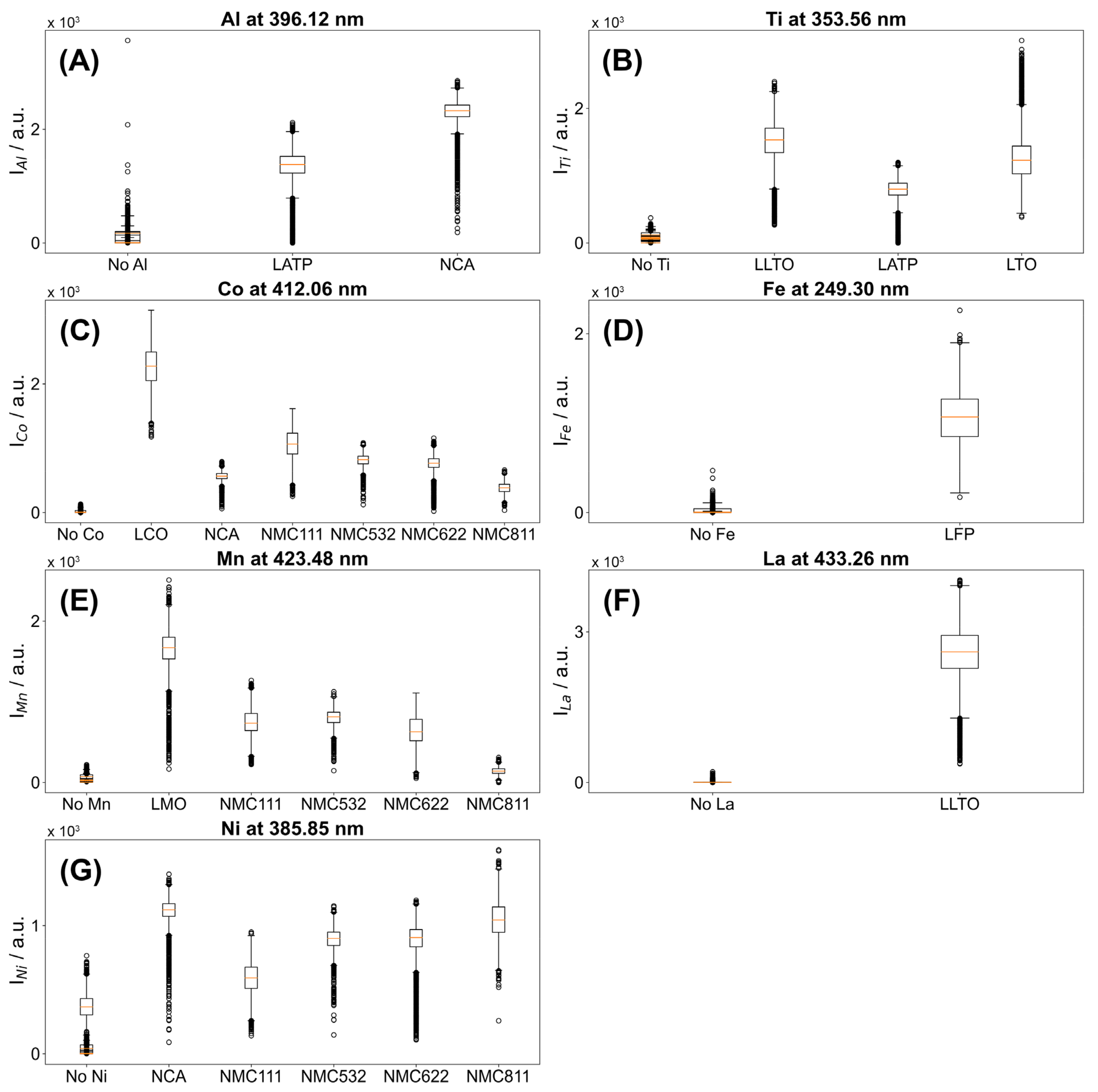
3.3. Specificity of Different Transition Lines

As a first step to understanding the data, it is important to choose emission lines with the best specificity and study whether classification is possible using a quantitative method. Different transitions based on qualitative observations, previous work, and the NIST database [30] were chosen to study the specificity of the elements contained in the analyzed materials. The selected transitions are put together in

Table 5. Selected transition lines of different battery materials.

Element	Transition/nm
Li	610.29
Al	396.12
Ti	353.56
Co	412.06
Fe	249.30
Mn	423.48
La	433.26
Ni	385.85

and are shown for visualization of the mean spectra of the different materials in Figure S1.

First, by comparing all the typical spectra for each material, single transition lines for seven elements were selected to investigate their specificity and linearity range. In Figure 5, different boxplots for each element are plotted to compare their intensity in non-bearing materials, according to the transition selected in Table 5. By looking at the chosen Ni, Mn, and Co line boxplots, good specificity is observed when comparing non-bearing materials to materials such as LCO, LMO, and NCA bearing higher contents of these targeted elements. For NMC111, NMC532, and NMC622, where Ni, Mn, and Co contents were more evenly distributed, the distribution of intensities was only a little wider than for non-bearing materials and their medians were less discernable than for more concentrated materials. The lines were chosen to the best of our knowledge regarding impurities and possible contamination affecting the specificity from overlapping lines; however, these results show that a method based on quantification and thresholding may not be enough to classify the different NMC compositions. For example, non-bearing Ni LFP material classification may become compromised if only based on Ni quantification because of the large amount of Fe transition lines in the Ni line wavelength range. For process analysis, this type of classification would be used to monitor NMC phase formation with precise ratios of Ni, Mn, and Co. To detect subtle phase changes, it is crucial to investigate algorithms even sturdier than a threshold method, due to the low specificity of the described lines. The Al boxplot shows narrow distributions, especially for the NCA material. Some non-Al-bearing materials showed higher Al contents. In this context, such a large distribution usually comes from contamination. Although precautions were taken, Al is an element abundantly used for parts in manufacturing processes. The lines for Fe, Ti, and La all showed the best specificity with a very narrow distribution of intensities in non-bearing materials. Of course, such observations are relative to the concentration of these elements in the materials. Furthermore, more materials bearing Fe and La should be analyzed to further discuss the specificity of the chosen lines. The LATP material showed wider distributions in Al and Ti boxplots. No overlap of each element’s lines was expected at these wavelength ranges, so some spectra acquisition either contained large particle size impurities or the laser was out of focus for some steps, perhaps due to the quality of the pellet or the particle size.

3.4. Linearity of Ni, Mn, and Co Transition Lines

Studying the linearity range of the different Ni, Mn, and Co transition lines was crucial, as saturation may result in a loss of accuracy during classification. In Figure 6, for example, the relative intensities of the Mn, Co, and Ni transitions for each material were plotted as a function of their expected contents. Curves with initial intensity values ((a), (b), and (c)) and values normalized over the Li transition line at 610.29 nm ((d), (e), and (f)) are provided to show the impact of normalizing signals by a sensitive transition on the calibration curves. Linearity was consequently better for normalized data. Although the Mn and Co lines seemed to be in the linear range when looking at their expected contents, the lack of data above 30 wt % and below about 60 wt % showed that no conclusions could be reached about the linearity range of such materials. Even if other LCO (Co: 60.2 wt%) and LMO (Mn: 60.8 wt%) samples were analyzed, other materials should be used to populate the 25 to 45 wt% range to reach conclusions on linearity and signal saturation. Furthermore, no conclusions could be reached for the Ni curve, shown in Figure 6B, as the distribution around the trend was wide. Although conclusions on whether the lines could be used to assess contents from typical calibration methods could not be made, the increased linearity when normalizing over the 610.29 nm Li transition line was promising and was thus used to normalize single transition lines in the next section.

3.5. Dimension Reduction at the Risk of Crucial Information Loss

The machine learning algorithms described earlier were first trained for classification using only a single transition line from the signal of seven elements composing the different materials analyzed. The train and validation set accuracy results at varying training set sizes are shown in

Table 6. Mean and RSD of accuracy using selected lines as inputs and using different machine learning algorithms over 10 iterations.

Algorithm		Train Set: 1% Test Set: 99%		Train Set: 5% Test Set: 95%		Train Set: 20% Test Set: 80%		Train Set: 50% Test Set: 50%
		Train Set	Validation Set	Train Set	Validation Set	Train Set	Validation Set	Train Set	Validation Set
AM	Mean accuracy/%	9.09	9.09	9.16	9.09	9.09	9.09	9.09	9.09
	RSD/%	<0.01	<0.01	0.02	<0.01	<0.01	<0.01	<0.01	<0.01
SVM	Mean accuracy/%	75.82	66.87	61.75	61.25	59.69	58.65	59.69	58.65
	RSD/%	0.06	0.11	0.09	0.08	0.03	0.06	0.04	0.05
RF	Mean accuracy/%	100.00	87.77	100.00	94.57	100.00	96.26	100.00	96.81
	RSD/%	<0.01	0.02	<0.01	0.01	<0.01	<0.01	<0.01	<0.01
DNN1	Mean accuracy/%	97.09	94.96	96.07	95.46	96.38	95.81	96.16	96.03
	RSD/%	0.02	<0.01	0.01	<0.01	0.01	<0.01	0.01	<0.01

. All results, including the testing set accuracy and training and testing times, are reported in Supplementary Material Tables S1–S4. Furthermore, confusion matrices for one iteration of each algorithm using a 0.01 train set size are shown in Figures S3–S6. Although the AM and SVM algorithms showed poor accuracy, results were improved using higher capacity RF and DNN1 algorithms. Although the results were improved, accuracies on the validation sets reached a maximum of about 97% when a large number of spectra was used for training, starting at about a 50% train set size or using about 250 spectra per sample for classification. This represented poor classification of NMC532, NMC622, and other similar classes, as observed in the confusion matrices. Overall, low-capacity AM showed poor accuracy results on unweighted results. Although AM was typically faster to compute, additional data pretreatment, such as individual scaling, should be done to improve results. Pretreatments are likely to increase computation times and require more user inputs or validation, which is not viable. The other tested algorithms showed poor accuracy, especially for the accurate classification of NMC532 and NMC622. Additionally, overfitting with the RF algorithm was clearly observed, as the accuracy on the training set is typically higher than the accuracy on the test set. Many solutions could be attempted to solve the overfitting issues of the RF algorithm. For example, the depth of the decision trees could be constrained or sturdier variational methods could be investigated. These solutions are not optimal for building databases subject to additions, because even if a constraining depth and other parameters are optimized for the current dataset, the same optimization work will have to be conducted again for other additions, which can be time-consuming and impractical as user inputs increase. One could choose to select multiple transition lines per element to extract more information and improve the classification task, but the same specificity and linear range validation task should also be performed, increasing the number of user inputs and making this validation method less robust. Therefore, we decided to try applying artificial intelligence algorithms on the full spectra to see whether avoiding information loss could solve both accuracy and overfitting issues.

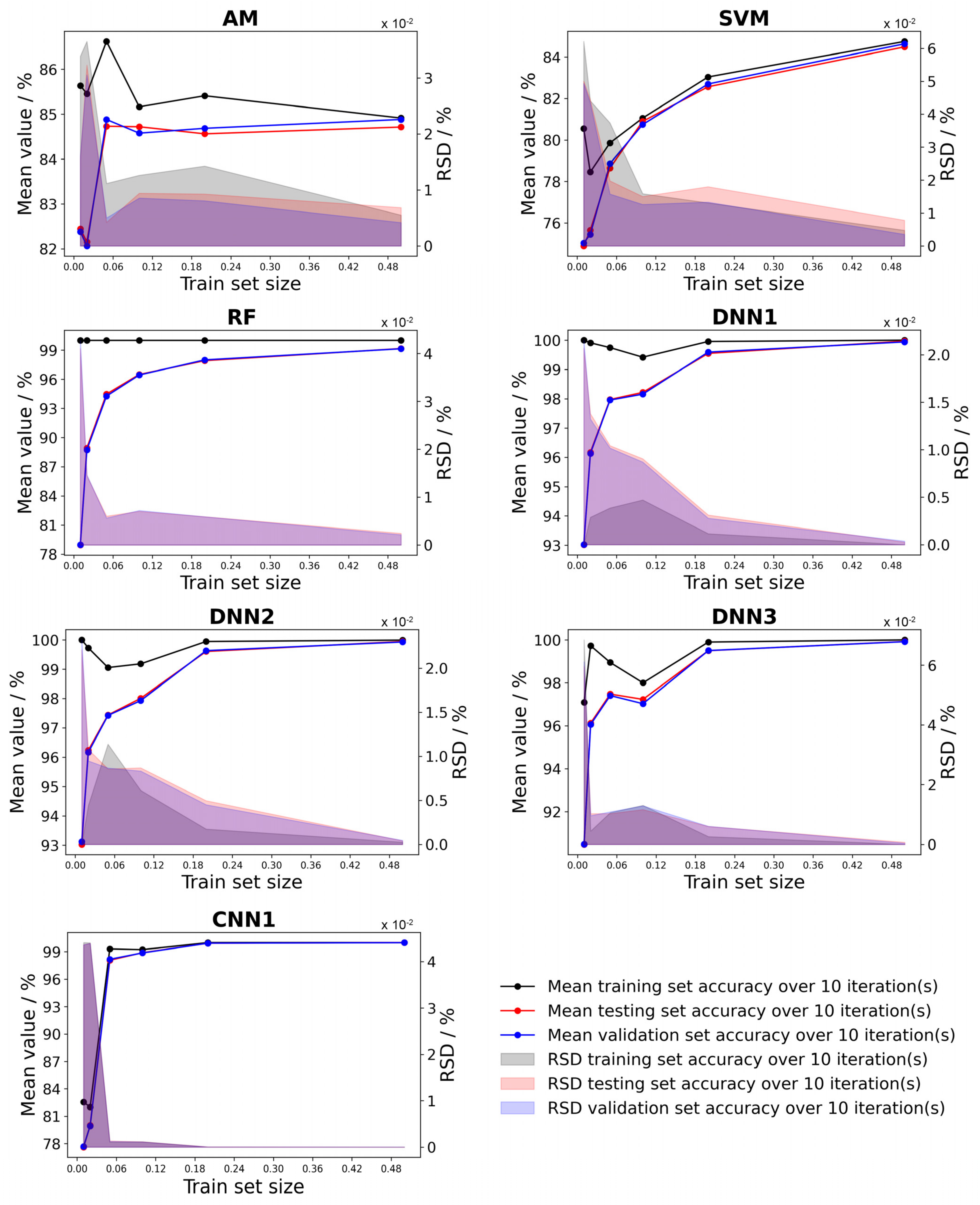
3.6. Deep Neural Network Classification

This time, using the full spectra, the same algorithms were used to classify the different battery materials. The results shown in

Table 7. Mean and RSD of accuracy using full spectra as inputs and different machine learning algorithms over 10 iterations.

Algorithm		Train Set: 1% Test Set: 99%		Train Set: 5% Test Set: 95%		Train Set: 20% Test Set: 80%		Train Set: 50% Test Set: 50%
		Train Set	Validation Set	Train Set	Validation Set	Train Set	Validation Set	Train Set	Validation Set
AM	Mean accuracy/%	85.64	82.38	86.62	84.88	85.41	84.68	84.91	84.88
	RSD/%	0.03	0.02	0.01	0.01	0.01	0.01	0.01	<0.01
SVM	Mean accuracy/%	80.55	75.04	79.85	78.86	83.04	82.70	84.75	84.63
	RSD/%	0.06	0.05	0.04	0.02	0.01	0.01	<0.01	<0.01
RF	Mean accuracy/%	100.00	78.97	100.00	94.27	100.00	97.99	100.00	99.14
	RSD/%	<0.01	0.04	<0.01	0.01	<0.01	0.01	<0.01	<0.01
DNN1	Mean accuracy/%	100.00	93.03	99.75	97.95	99.95	99.59	100.00	99.94
	RSD/%	<0.01	0.02	<0.01	0.01	<0.01	<0.01	<0.01	<0.01
DNN2	Mean accuracy/%	100.00	93.12	99.05	97.42	99.95	99.63	99.99	99.63
	RSD/%	<0.01	0.02	0.01	0.01	<0.01	<0.01	<0.01	<0.01
DNN3	Mean accuracy/%	97.09	90.49	98.95	97.41	99.90	99.50	100.00	99.92
	RSD/%	0.07	0.06	0.01	0.01	<0.01	0.01	<0.01	<0.01
CNN1	Mean accuracy/%	82.55	77.68	99.31	98.18	100.00	99.94	100.00	99.99
	RSD/%	0.44	0.44	0.01	0.01	<0.01	<0.01	<0.01	<0.01

were computed on spectra normalized to their norm. All results, including the testing set accuracy and training and testing times, are reported in Supplementary Material Tables S5–S11. Furthermore, confusion matrices for one iteration of each algorithm using a 0.01 train set size are shown in Figures S7–S13. At the microscopic scale, pellets had a rough surface; thus, when normalized to their norm, out-of-focus pixels introduced more noise to patterns at scales similar to in-focus samples. Furthermore, a norm normalization described in Equation (1) was performed instead of mean normalization because all the algorithms tested besides AM were parametric. This meant the data needed to classify new spectra were only parameters; neither the training files nor mean spectra were needed. This was a useful asset as the training time was not affected by the number of spectra used for training and checkpoint files are typically smaller than hyperspectral data saved for non-parametric algorithms.

In Table 7, AM and SVM again exhibit poor, yet improved, accuracy results. RF and DNN1 were also improved by avoiding the loss of information using full spectra. Although these results improved, overfitting was still observed using RF and DNN1, especially when using fewer spectra for the training. In Figure 7, for example, accuracies and RSD for a higher number of training set sizes are plotted for the different machine learning algorithms (1, 2, 5, 10, 20, and 50%). Overfitting using AM and RF is clearly noticeable, whereas SVM shows no such issue. DNN1 is trickier, overfitting at 1, 2, and 5%, but showing slightly lesser accuracy, and less overfitting at 10%. Overfitting in LIBS spectra manifests itself either by fitting to the background noise or fitting to trace elements, such as Na, K, or Ca, for which LIBS has high sensitivity and detects low ppm/high ppb. If trace element contents were somewhat homogenous in a few materials, this signal could be interpreted by the algorithm as being a feature important for classification. The goal of the overfitting study was to mitigate the use of non-specific signals and favorably use the signal of composing elements. An application of the phase specificity of the LIBS signal was to distinguish even smaller stoichiometric changes, such as (de)lithiation upon cycling. For such an application, fewer spectra were predicted to be available to train the different algorithms; thus, another objective was to improve the accuracy of the test set for smaller train set sizes.

One approach to take better advantage of the complete set of inputs was to use deep learning architectures with enough capacity. The definition of deep learning is similar to neural networks, but layers are juxtaposed into so-called hidden layers. Unique architectures can be created, including CNN, with the goal to increase the number of extracted features and have better control over the bias–variance trade-off. Two simple deep learning architectures were tested, first using two (DNN2), then three (DNN3) hidden layers. Better accuracy and less overfitting were obtained using DNN3 at a 10% training set size, shown in Figure 7, demonstrating the potential of feature extraction on variance reduction and overfitting for accurate classification. Finally, a CNN architecture based on convolution and pooling parameters reported by Zhao et al. [29] (CNN1) exhibited promising results.

An accuracy of 99.18% at 5% was the highest score using any algorithm. Furthermore, although accuracy scores at 1 and 2% were lower than using DNN2 and DNN3, much less overfitting was observed, and the uncertainty on the classification of the test set was more coherent with the steady accuracy increase with the increase in training set size. Another promising result was the improved overfitting on smaller training sets using the CNN1 algorithm. The accuracy on both training and testing sets at 1% was of interest for this methodology. Out of ten iterations, the CNN1 algorithm should have been trained longer and/or with a smaller learning rate for one or a few of the iterations, but in general, showed good accuracies, as shown in the confusion matrix in Figure S13. The uncertainty of the results was interesting to add to a methodology to automatically optimize deep learning algorithm parameters when executed by an inexperienced user. Although the learning rate and patience parameters were enough to obtain good results for bigger training sets, the uncertainty at 1% foreshadows that training parameters may result in some errors, even though CNN1 had promising results overall.

3.7. Training and Testing Times

More consideration is needed for the different training and testing times using different data pretreatment and algorithms. Data is available in supporting information, along with mean time values and RSD, using full normalized spectra as inputs. Training times for deep learning algorithms (DNN1, DNN2, DNN3, and CNN1) were not optimized for the task: the number of epochs, patience, and learning rates can be tuned to lower computation times. As the algorithms were tested for multiple iterations, the number of epochs was set at 500 to ensure training reached a minimal loss at each iteration. Therefore, the reader should consider training time tendencies as the number of training data increases and testing times. In Figure S14, deep learning algorithm training times are less affected by the training set size than AM, SVM, and RF, which shows that for large datasets, and thus hyperspectral data, deep learning parametric algorithms exhibit more fine-tuning potential. Furthermore, testing times of deep learning algorithms were the same order of magnitude as RF and SVM algorithms, even for the CNN1, which could have been expected to be more time-consuming due to the convolution step. Deep learning algorithms, although taking longer to train using unoptimized parameters, showed good composition classification capabilities at testing times similar to the RF algorithm, exhibiting competitive accuracy results. In settings such as quality control or synthesis composition validation, the algorithms would already be trained, so that the training times affect real-time analysis less than testing times.

Overall, considering the training and testing times and accuracy results, deep learning algorithms showed a better capability in adapting to the needs of the task. Depending on the amount of training data available, its variance, and computational needs, the chosen algorithm can be engineered to offer an inexperienced user in-depth solutions to the task to be performed. The methodology presented in this paper is thus pioneering the uniformization of different algorithm performances, which can be applied to different tasks and run by users from different backgrounds. Although training parameters can be tuned for the task, the ultimate automated system should be able to independently assess whether the training is being performed with optimal parameters; however, there are no studies or methodologies currently in the literature to tackle chemical analytics.

4. Conclusions

To conclude, the specific measurement of different NMC cathode material compositions and other Li-ion battery materials was studied, along with a validation method first investigating transition line specificity and linear range, and then using different artificial intelligence algorithms for classification. Overall, a CNN deep learning algorithm allowed for improved control on overfitting and better accuracy results using fewer spectra for training. Depending on the training sets and computing apparatus available, one could choose a simpler deep learning architecture to lower training computation times. The use of artificial intelligence on digitalized data is versatile and can be used to improve the identification of components and even compositions, depending on the target applications. Real-time applications using deep learning algorithms would be possible, as testing times took about 1.5 s for 11 000 spectra, or 0.2 ms per spectrum, which is the same order of magnitude as CORIOSITY LIBS acquisition rates. Considering the fast computational development and parallel computing, deep learning methods appear to be a realistic solution for improving the accuracy of different classification or regression tasks and will allow better methodologies in the future for inexperienced users to execute a training task, such as in quality control laboratory settings.

Li-ion battery manufacturing and recycling processes can thus be improved and made safer by robotizing (dis)assembly, which relies greatly on real-time digitalization. Elemental compositions vary from different manufacturers and products, and manufacturing a chemical sensor capable of accurately identifying compositions fast, with high accuracy and good sensitivity to lithium contents, would increase the efficiency of recycling processes.

This study demonstrates the capability of a high-throughput LIBS instrument to accurately classify different Li-ion battery components from different manufacturers at record speeds of 0.77 ms/pixel. As opposed to other techniques used in the , such as XRD and XPS, LIBS has a higher throughput, requires no sample preparation, and has no special conditions, such as vacuum or vector gases. Furthermore, the sensitivity to and direct analysis of Li contents is exemplary and allows the study of new metrics, such as elemental distributions. Although this performance is innovative and may solve several quality control issues, the reader should keep in mind that LIBS is an ablation method; thus, applications are limited to post-cycling studies. LIBS shows much better practicability than induced-coupled plasma methods used for recycling and manufacturing, and its spatial information allows for better sampling logistics, as a LIBS sensor could be placed on a conveyor belt or anywhere on the process line to assess real-time contents and compositions. Future work to investigate trace element contents and distributions and classify smaller stoichiometric changes, such as the (de)lithiation of the same composition of the same material, would provide further insight for battery materials manufacturers and academic researchers on using the LIBS signal to characterize synthetic materials.

References

1. Zhu, Z.; Jiang, T.; Ali, M.; Meng, Y.; Jin, Y.; Cui, Y.; Chen, W. Rechargeable Batteries for Grid Scale Energy Storage. Chem. Rev. 2022. [Google Scholar] [CrossRef] [PubMed]
2. Zhou, L.; Garg, A.; Zheng, J.; Gao, L.; Oh, K.Y. Battery pack recycling challenges for the year 2030: Recommended solutions based on intelligent robotics for safe and efficient disassembly, residual energy detection, and secondary utilization. Energy Storage 2020, 3, e190. [Google Scholar] [CrossRef]
3. Lu, Y.; Han, X.; Li, Z. Enabling Intelligent Recovery of Critical Materials from Li-Ion Battery through Direct Recycling Process with Internet-of-Things. Materials 2021, 14, 7153. [Google Scholar] [CrossRef] [PubMed]
4. Paradis, M.-C.M.; Doucet, F.R.; Rifai, K.; Özcan, L.Ç.; Azami, N.; Vidal, F. ECORE: A New Fast Automated Quantitative Mineral and Elemental Core Scanner. Minerals 2021, 11, 859. [Google Scholar] [CrossRef]
5. Rifai, K.; Michaud Paradis, M.-C.; Swierczek, Z.; Doucet, F.; Özcan, L.; Fayad, A.; Li, J.; Vidal, F. Emergences of New Technology for Ultrafast Automated Mineral Phase Identification and Quantitative Analysis Using the CORIOSITY Laser-Induced Breakdown Spectroscopy (LIBS) System. Minerals 2020, 10, 918. [Google Scholar] [CrossRef]
6. Rifai, K.; Constantin, M.; Yilmaz, A.; Özcan, L.Ç.; Doucet, F.R.; Azami, N. Quantification of Lithium and Mineralogical Mapping in Crushed Ore Samples Using Laser Induced Breakdown Spectroscopy. Minerals 2022, 12, 253. [Google Scholar] [CrossRef]
7. Pamu, R.; Davari, S.A.; Darbar, D.; Self, E.C.; Nanda, J.; Mukherjee, D. Calibration-Free Quantitative Analysis of Lithium-Ion Battery (LiB) Electrode Materials Using Laser-Induced Breakdown Spectroscopy (LIBS). ACS Appl. Energy Mater. 2021, 4, 7259–7267. [Google Scholar] [CrossRef]
8. Imashuku, S.; Taguchi, H.; Kawamata, T.; Fujieda, S.; Kashiwakura, S.; Suzuki, S.; Wagatsuma, K. Quantitative lithium mapping of lithium-ion battery cathode using laser-induced breakdown spectroscopy. J. Power Sources 2018, 399, 186–191. [Google Scholar] [CrossRef]
9. Smyrek, P.; Zheng, Y.; Rakebrandt, J.-H.; Seifert, H.J.; Pfleging, W. Investigation of Micro-Structured Li(Ni1/3Mn1/3Co1/3)O2 Cathodes by Laser-Induced Breakdown Spectroscopy. In Proceedings of the SPIE LASE, San Francisco, CA, USA, 17 February 2017. [Google Scholar] [CrossRef]
10. Smyrek, P.; Bergfeldt, T.; Seifert, H.J.; Pfleging, W. Laser-induced breakdown spectroscopy for the quantitative measurement of lithium concentration profiles in structured and unstructured electrodes. J. Mater. Chem. A 2019, 7, 5656–5665. [Google Scholar] [CrossRef]
11. Smyrek, P.; Pröll, J.; Seifert, H.J.; Pfleging, W. Laser-Induced Breakdown Spectroscopy of Laser-Structured Li(NiMnCo)O2Electrodes for Lithium-Ion Batteries. J. Electrochem. Soc. 2015, 163, A19–A26. [Google Scholar] [CrossRef]
12. Smyrek, P.; Zheng, Y.; Seifert, H.J.; Pfleging, W. Post-mortem characterization of fs laser-generated micro-pillars in Li(Ni1/3Mn1/3Co1/3)O2 electrodes by laser-induced breakdown spectroscopy. In Proceedings of the SPIE LASE, San Francisco, CA, USA, 18 March 2016. [Google Scholar] [CrossRef]
13. Zorba, V.; Syzdek, J.; Mao, X.; Russo, R.E.; Kostecki, R. Ultrafast laser induced breakdown spectroscopy of electrode/electrolyte interfaces. Appl. Phys. Lett. 2012, 100, 234101. [Google Scholar] [CrossRef]
14. Zheng, Y.; Pfäffl, L.; Seifert, H.J.; Pfleging, W. Lithium Distribution in Structured Graphite Anodes Investigated by Laser-Induced Breakdown Spectroscopy. Appl. Sci. 2019, 9, 4218. [Google Scholar] [CrossRef] [Green Version]
15. Imashuku, S.; Taguchi, H.; Fujieda, S.; Suzuki, S.; Wagatsuma, K. Three-dimensional lithium mapping of graphite anode using laser-induced breakdown spectroscopy. Electrochim. Acta 2019, 293, 78–83. [Google Scholar] [CrossRef]
16. Hou, H.; Cheng, L.; Richardson, T.; Chen, G.; Doeff, M.; Zheng, R.; Russo, R.; Zorba, V. Three-dimensional elemental imaging of Li-ion solid-state electrolytes using fs-laser induced breakdown spectroscopy (LIBS). J. Anal. At. Spectrom. 2015, 30, 2295–2302. [Google Scholar] [CrossRef]
17. Peng, L.; Sun, D.; Su, M.; Han, J.; Dong, C. Rapid analysis on the heavy metal content of spent zinc–manganese batteries by laser-induced breakdown spectroscopy. Opt. Laser Technol. 2012, 44, 2469–2475. [Google Scholar] [CrossRef]
18. Costa, V.C.; de Mello, M.L.; Babos, D.V.; Castro, J.P.; Pereira-Filho, E.R. Calibration strategies for determination of Pb content in recycled polypropylene from car batteries using laser-induced breakdown spectroscopy (LIBS). Microchem. J. 2020, 159, 105558. [Google Scholar] [CrossRef]
19. Meima, J.A.; Rammlmair, D. Investigation of compositional variations in chromitite ore with imaging Laser Induced Breakdown Spectroscopy and Spectral Angle Mapper classification algorithm. Chem. Geol. 2020, 532, 119376. [Google Scholar] [CrossRef]
20. Han, L.; Liu, F.; Zhang, L. An Improved Sub-Model PLSR Quantitative Analysis Method Based on SVM Classifier for ChemCam Laser-Induced Breakdown Spectroscopy. Symmetry 2021, 13, 319. [Google Scholar] [CrossRef]
21. Yang, H.-X.; Fu, H.-B.; Wang, H.-D.; Jia, J.-W.; Sigrist, M.W.; Dong, F.-Z. Laser-induced breakdown spectroscopy applied to the characterization of rock by support vector machine combined with principal component analysis. Chin. Phys. B 2016, 25, 065201. [Google Scholar] [CrossRef]
22. Janovszky, P.; Jancsek, K.; Palásti, D.J.; Kopniczky, J.; Hopp, B.; Tóth, T.M.; Galbács, G. Classification of minerals and the assessment of lithium and beryllium content in granitoid rocks by laser-induced breakdown spectroscopy. J. Anal. At. Spectrom. 2021, 36, 813–823. [Google Scholar] [CrossRef]
23. Koujelev, A.; Sabsabi, M.; Motto-Ros, V.; Laville, S.; Lui, S.L. Laser-induced breakdown spectroscopy with artificial neural network processing for material identification. Planet. Space Sci. 2010, 58, 682–690. [Google Scholar] [CrossRef]
24. Yang, Y.; Li, C.; Liu, S.; Min, H.; Yan, C.; Yang, M.; Yu, J. Classification and identification of brands of iron ores using laser-induced breakdown spectroscopy combined with principal component analysis and artificial neural networks. Anal. Methods 2020, 12, 1316–1323. [Google Scholar] [CrossRef]
25. Chen, J.; Pisonero, J.; Chen, S.; Wang, X.; Fan, Q.; Duan, Y. Convolutional neural network as a novel classification approach for laser-induced breakdown spectroscopy applications in lithological recognition. Spectrochim. Acta Part B At. Spectrosc. 2020, 166, 105801. [Google Scholar] [CrossRef]
26. Chen, T.; Sun, L.; Yu, H.; Wang, W.; Qi, L.; Zhang, P.; Zeng, P. Deep learning with laser-induced breakdown spectroscopy (LIBS) for the classification of rocks based on elemental imaging. Appl. Geochem. 2022, 136, 105135. [Google Scholar] [CrossRef]
27. Li, L.-N.; Liu, X.-F.; Xu, W.-M.; Wang, J.-Y.; Shu, R. A laser-induced breakdown spectroscopy multi-component quantitative analytical method based on a deep convolutional neural network. Spectrochim. Acta Part B At. Spectrosc. 2020, 169, 105850. [Google Scholar] [CrossRef]
28. Castorena, J.; Oyen, D.; Ollila, A.; Legget, C.; Lanza, N. Deep spectral CNN for laser induced breakdown spectroscopy. Spectrochim. Acta Part B At. Spectrosc. 2021, 178, 106125. [Google Scholar] [CrossRef]
29. Zhao, W.; Li, C.; Yan, C.; Min, H.; An, Y.; Liu, S. Interpretable deep learning-assisted laser-induced breakdown spectroscopy for brand classification of iron ores. Anal. Chim. Acta 2021, 1166, 338574. [Google Scholar] [CrossRef]
30. Kramida, A.; Ralchenko, Y.; Reader, J. NIST Atomic Spectra Database (ver. 5.9); NIST: Gaithersburg, MD, USA, 2021. [Google Scholar] [CrossRef]
Figure 1. A CORIOSITY LIBS instrument by ELEMISSION.
Batteries 08 00231 g001
Figure 2. LIBS mean spectra of all the battery materials analyzed using the described method between 215 and 940 nm.
Batteries 08 00231 g002
Figure 3. LIBS mean spectra of NMC532 and NMC622 between: (A) 215 and 415 nm and (B) 335 and 365 nm.
Batteries 08 00231 g003
Figure 4. (A) Intensities and (B) relative standard deviations of Li lines at 610.29, 670.81, and 812.65 nm in LIBS spectra of different battery materials.
Batteries 08 00231 g004
Figure 5. Boxplot of the intensities of (A) Al, (B) Ti, (C) Co, (D) Fe, (E) Mn, (F) La, and (G) Ni emission lines in different materials.
Batteries 08 00231 g005
Figure 6. Intensities of (A) Co, (B) Mn, and (C) Ni emission lines with background removal and (D) Co, (E) Mn, and (F) Ni emission lines relative to Li at 610.29 nm as functions of their expected contents in different battery materials.
Batteries 08 00231 g006
Figure 7. Accuracy and RSD as functions of the training set size for different machine learning classification algorithms over 10 iterations, using full spectra.
Batteries 08 00231 g007