Article

Uncertainty-Aware Lightweight Design of CFRP Battery Enclosure Under Extreme Cold Side-Pole Impact via Bayesian Surrogates


1
College of Automobile and Traffic Engineering, Heilongjiang Institute of Technology, Harbin 150050, China
2
College of Mechanical and Electronic Engineering, East University of Heilongjiang, Harbin 150066, China
*
Author to whom correspondence should be addressed.
Batteries 2026, 12(2), 61; https://doi.org/10.3390/batteries12020061
Submission received: 26 January 2026 / Revised: 5 February 2026 / Accepted: 12 February 2026 / Published: 13 February 2026
(This article belongs to the Section Battery Processing, Manufacturing and Recycling)

Abstract

Mass M (kg) and peak intrusion L (mm) are jointly minimized for a CFRP-enabled battery pack enclosure under the GB 38031-2025 −40° side-pole extrusion condition. A 50-run explicit FE design of experiments is conducted and deterministically partitioned into 37/5/5/3 for initial training, two sequential enrichment batches, and an independent hold-out test. Bayesian additive regression trees are trained as the primary surrogates for M, L, and Stress, and stress acceptability is enforced through a probability-of-feasibility (PoF) gate anchored to a baseline-scaled cap, σlim = 1.2 σbase = 410.4 MPa. NSGA-II performed on the feasible surrogate landscape yields a bimodal feasible non-dominated set. The two branches correspond to two discrete levels of a key thickness variable x4: a low-mass regime (n = 106) with M = 100.61–104.81 kg and L = 5.430–5.516 mm at x4 ≈ 5.60 mm, and a stiffer regime (n = 94) with M = 110.69–115.08 kg and L = 5.362–5.430 mm at x4 ≈ 8.00 mm. PoF screening eliminates part of the intermediate region where feasibility confidence is insufficient. Independent FE reruns further indicate that the PoF gate reduces deterministic misclassification near the stress boundary (e.g., one near-threshold candidate exceeds σlim, whereas others satisfy the cap with margin). Overall, the proposed workflow offers a traceable lightweighting route under extreme-cold uncertainty within a constrained FE budget.

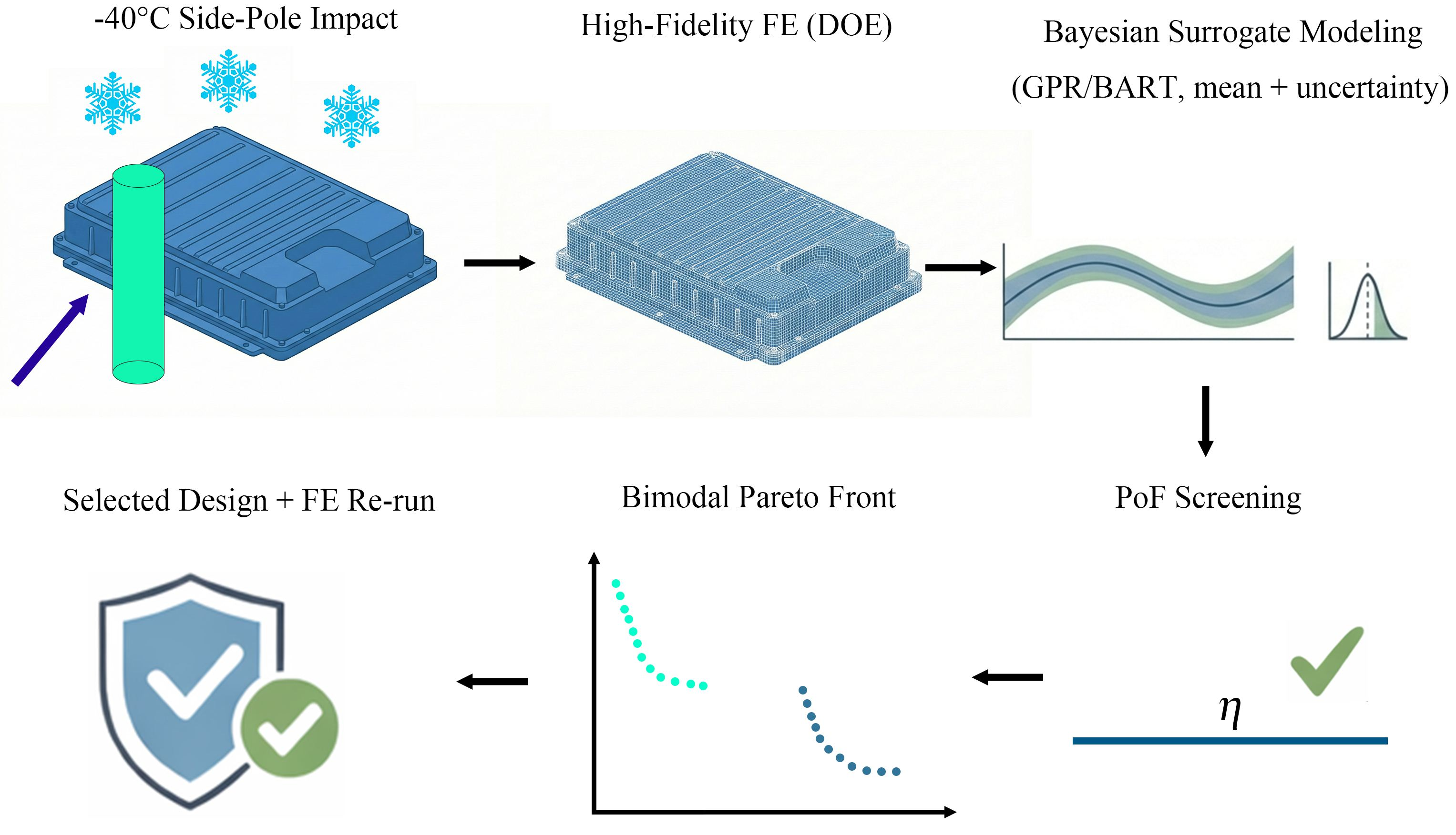
Graphical Abstract

1. Introduction

Operating battery electric vehicles in cold regions imposes stricter requirements on the structural safety and reliability of the battery pack enclosure. Low temperatures can substantially alter the mechanical response and failure mechanisms of polymer-matrix constituents and laminated composites. In particular, reduced matrix ductility and temperature-dependent damage evolution may promote crack initiation and interlaminar/interfacial growth, thereby changing energy-absorption pathways and degrading intrusion resistance under pole-type loading [1,2].
At the regulatory level, tightening safety requirements further amplify the need for early-stage, structure-level verification. China’s mandatory national standard GB 38031—2025 has been released with a defined implementation schedule [3], and its official listing specifies the release date and the enforcement date (1 July 2026) [3], reinforcing the expectation that traction-battery systems satisfy stringent safety criteria under prescribed conditions [4].
Among side-pole crash and intrusion scenarios, stress acceptability is enforced via a probabilistic feasibility gate calibrated to a baseline-scaled stress threshold, which governs both the adaptive enrichment and candidate filtering processes. Excessive structural intrusion constitutes the primary precipitating factor for mechanical abuse-induced thermal runaway in traction batteries. Consequently, confining deformation within the available packaging clearance is paramount to preclude module compression and subsequent internal short circuits (ISCs). Representative protocols prescribe a rigid, narrow pole and tightly defined impact kinematics; for example, the Euro NCAP oblique pole protocol specifies a target speed of 32 km/h and a 75° impact angle, while the U.S. compliance procedure for FMVSS 214 rigid-pole testing standardizes key requirements for the vehicle-to-pole configuration. Such narrow-pole loading can trigger rapid local buckling and high curvature deformation in sills, cross-members, and battery-side walls, motivating battery-protection concepts and dedicated energy-absorbing modules tailored to lateral pole loading [4,5,6,7,8].
Lightweighting strategies often consider CFRP-based solutions because of their high specific stiffness and strength; however, cold-region applications face a practical obstacle: low-temperature material data are “available but not self-consistent.” Beyond the commonly cited low-temperature static/impact studies, additional work has quantified temperature effects on tensile behavior and impact damage characteristics and has reported residual strength after impact at low temperatures, collectively indicating that measured trends depend strongly on the specific fiber/resin system, layup, cure route, and test metric [9,10,11]. Consequently, building a fully consistent, full-temperature coupon database is often cost-prohibitive, whereas assembling parameters across heterogeneous sources can introduce system-mismatch uncertainty that undermines simulation fidelity and design conclusions [12,13]. Given the prohibitive logistics of comprehensively characterizing every layup candidate at −40 °C, deterministic optimization is prone to yielding non-robust designs. Consequently, a paradigm shift is essential: rather than presuming the availability of exhaustive empirical data, the design framework must explicitly internalize the predictive uncertainty inherent in sparse or heterogeneous material inputs.
Computational cost forms a second bottleneck. Side pole crash simulations are commonly performed using explicit dynamics, where the stable time increment is constrained by the smallest characteristic element length and the dilatational wave speed; mesh refinement in contact and local buckling regions can therefore reduce the critical time step and inflate runtime. When the design space includes multiple geometric and laminate variables and the assessment must be repeated under multiple temperature scenarios, direct high-fidelity simulation-driven multi-objective exploration becomes prohibitively expensive. Recent work has therefore pursued high-throughput virtual crash datasets and machine-learning surrogates to accelerate crashworthiness screening under side-pole-type loading, while Bayesian optimization and sequential sampling provide a principled route to reduce the number of expensive evaluations under uncertainty [14,15,16,17].
Recent work has addressed lateral crash protection for EV battery enclosures, including pole-impact-oriented energy absorbers and enclosure-level crashworthiness concepts under pole-type loading [5]. In parallel, surrogate and machine-learning models have been explored to accelerate crashworthiness assessment when high-fidelity explicit simulations are expensive [14,18,19,20]. System-level battery-pack models implemented in MATLAB/Simulink have also been reported for electrical-performance studies. These models complement structure-level crashworthiness simulations [21]. Meanwhile, composite mechanics studies have consistently reported that CFRP mechanical response and damage evolution can change markedly with temperature, including low-temperature static behavior and impact-induced damage characteristics.
However, these lines of research are rarely combined into a reusable workflow for cold-region enclosure design under side-pole extrusion. First, enclosure-level studies commonly assume generic or room-temperature conditions, while low-temperature effects are often examined at coupon/laminate level without being propagated to enclosure-level extrusion response and design decisions. Second, low-temperature composite inputs available in the literature are fragmented across material systems, layups, and test definitions; directly assembling parameters from multiple sources can introduce hidden inconsistencies, yet such system-mismatch uncertainty is seldom represented in a traceable manner. Third, explicit pole-impact analyses remain computationally demanding due to stability-limited time increments and local mesh refinement near contact/buckling regions, which makes brute-force multi-objective exploration impractical under realistic budgets. Finally, credibility loops are often limited to internal surrogate validation; independent high-fidelity reruns at selected designs (and scaled verification when feasible) are important to support safety-relevant conclusions [14].
To address these limitations, the present study adopts −40 °C as the primary scenario and establishes a traceable, uncertainty-aware, and sample-efficient surrogate-assisted workflow for side-pole extrusion design of battery pack enclosures [15].
In summary, this workflow integrates low-temperature composite uncertainty, feasibility-aware optimization, and independent FE reruns to enable reliable lightweight design under a tight simulation budget.

2. Materials and Methods

2.1. FE Model and Side-Pole Extrusion Setup

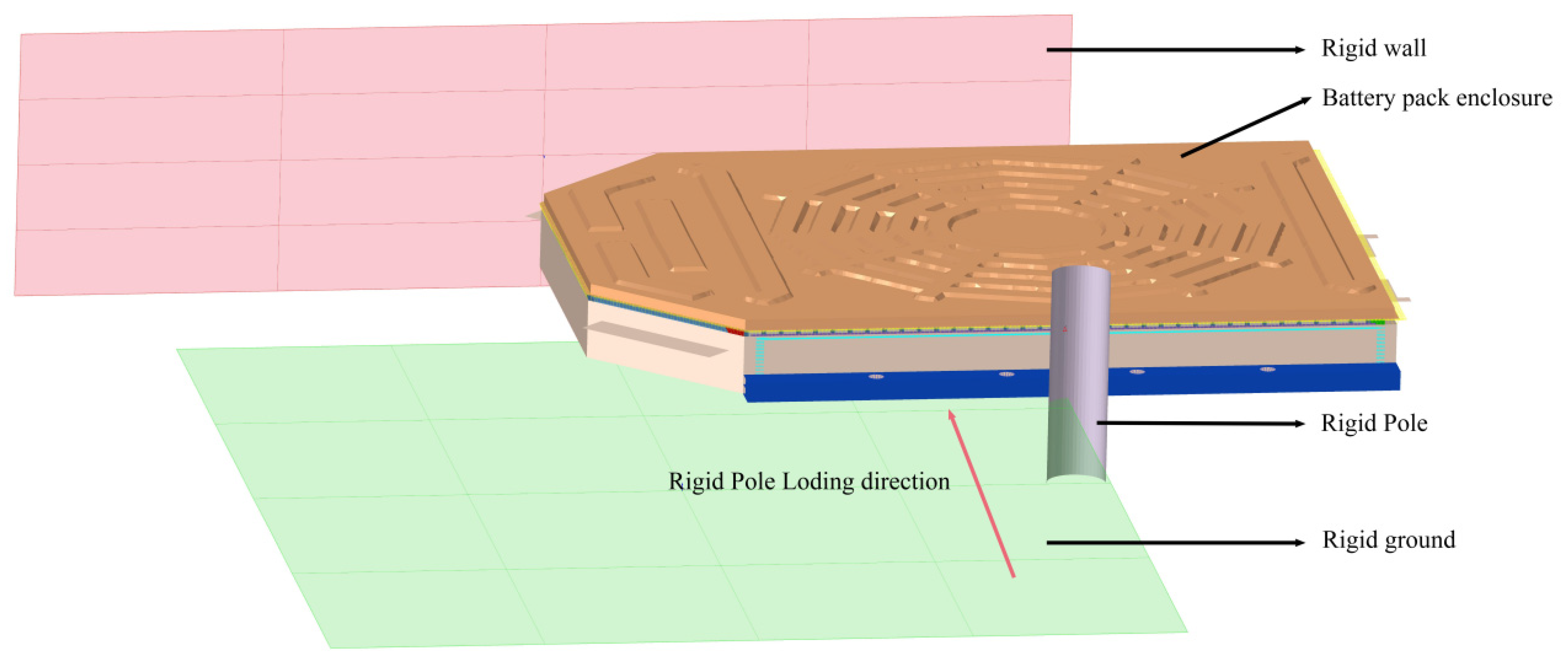
Lateral extrusion evaluates the crush resistance of the battery pack enclosure. It also reduces the risk of cell/module squeezing during collapse. The simulation follows GB 38031-2025, §8.2.4. After extrusion, the pack/system must show no fire or explosion. The post-test insulation resistance must meet the standard requirements. Figure 1 shows the assembly-level model. Two rigid walls constrain the assembly. A rigid cylindrical pole loads the long-side surface of the enclosure.
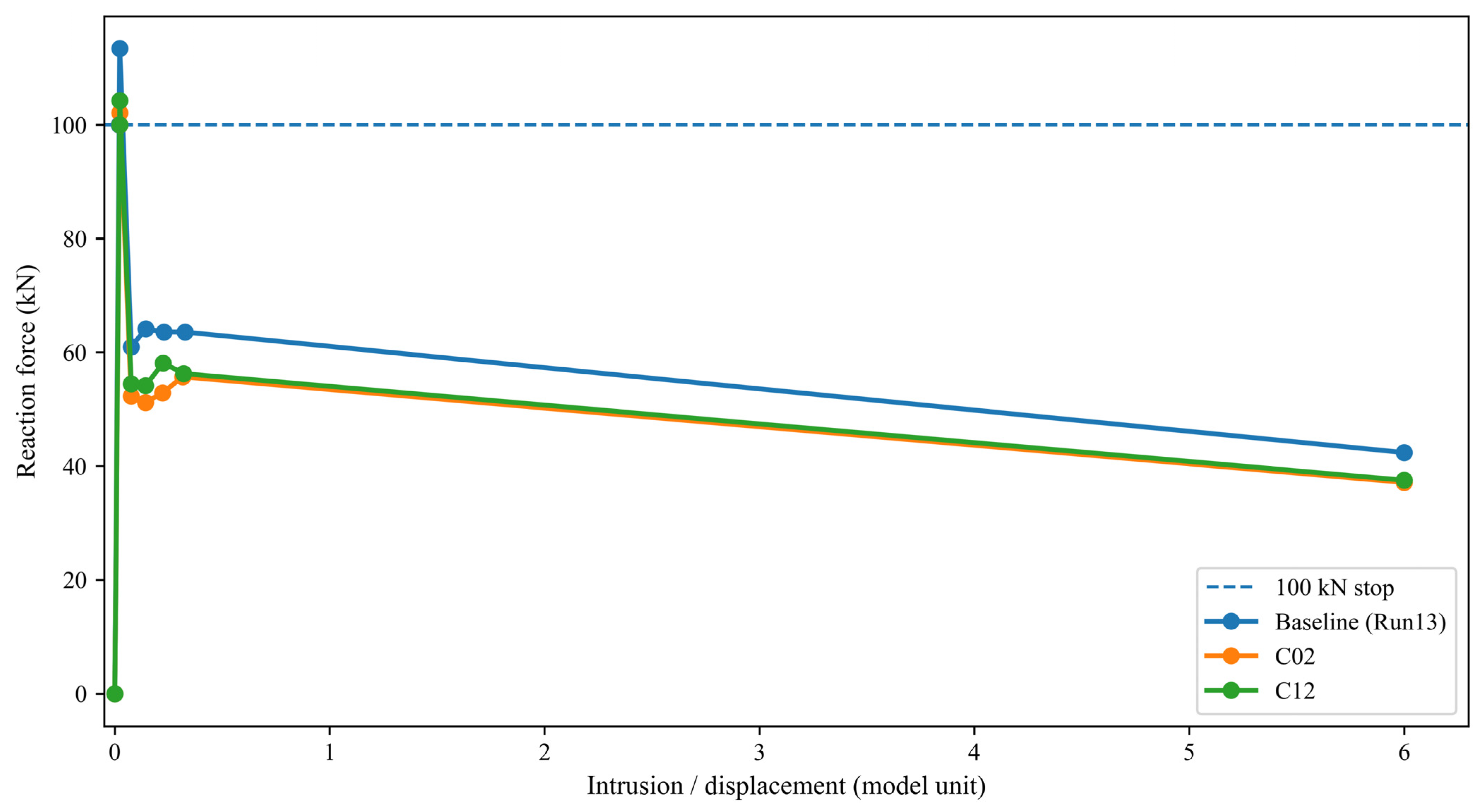
A rigid cylindrical pole (150 mm in diameter) moves in the −Z direction under displacement control at 2 mm/s. Loading stops when the reaction force reaches 100 kN. It also stops if deformation reaches 30% of the overall dimension in the loading direction. The earlier condition is used. The standard specifies a 10 min hold at the final displacement. Here, responses are extracted only up to the termination point [6,7].
The enclosure is discretized mainly with shell elements. The nominal element size is 10 mm in the production runs. This size resolves the pole–beam contact region. Numerical stability is checked using commonly energy-balance criteria. Beam-to-case connections use nodal coupling. Skin–core bonding uses TIE constraints. Pole–enclosure interaction uses surface-to-surface contact. A soft-contact formulation is applied (SOFT = 1). Penetration controls are kept consistent.
Key numerical settings are summarized for reproducibility. Shell elements are used. The global −Z axis is the extrusion direction. Shell formulation, through-thickness integration, and hourglass control follow LS-DYNA R11.0 explicit settings. These options are fixed in all cases. The loading rate is 2 mm/s to limit inertial effects. Contact uses a penalty-based surface-to-surface formulation with SOFT = 1. Friction and penetration controls are identical in all runs. Rigid walls suppress rigid-body motion. Mounting constraints follow the baseline installation definition.
Besides the standard pass/fail safety criteria, an application-oriented protection constraint is imposed based on the packaging layout: the maximum intrusion L in the loading direction shall be smaller than the 20 mm packaging clearance between the enclosure and the internal modules. Accordingly, the total enclosure mass M, the maximum intrusion L, and the peak equivalent stress in the enclosure are reported as the key performance metrics for subsequent evaluation and optimization.

2.2. Design Variables, Objectives, and Constraints

2.2.1. Variables and Bounds

Let x denote the design vector. To keep the extreme-cold campaign computationally affordable, the parameterization is limited to a small set of factors that directly control the main load paths, while secondary details are held constant at baseline settings.
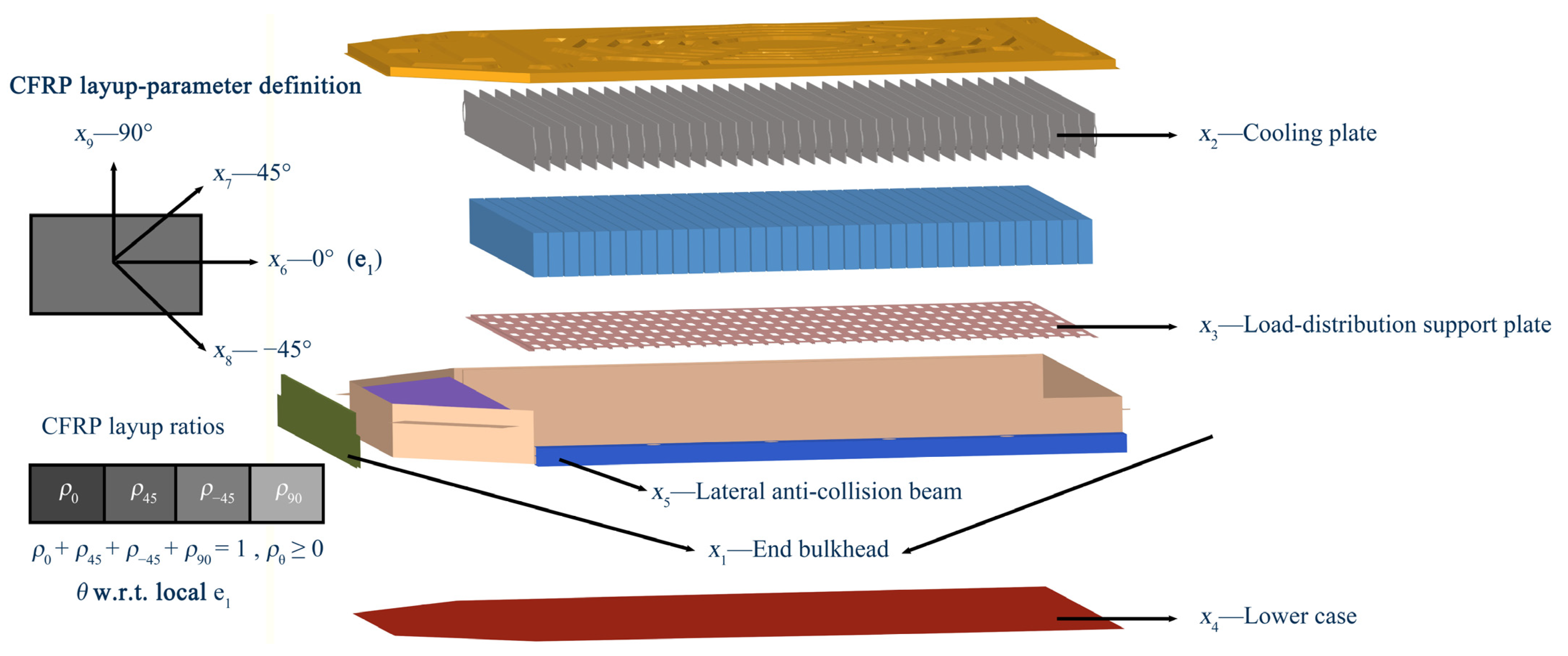
As shown in Figure 2, the design variables are described as follows:
x = x 1 , , x 9 T
The first five variables x1x5 (mm) are thicknesses assigned to the end bulkhead, cooling plate, load-distribution support plate, lower case, and lateral anti-collision beam, respectively.
The remaining four variables x6, x7, x8, and x9 describe the CFRP layup using an orientation-grouped weight parameterization for 0°, +45°, −45°, and 90° plies. Ply angles are defined with respect to the local e1 axis in Figure 1. To obtain physically meaningful layup ratios with a unit sum, the weights are normalized prior to laminate construction as follows:
r i = x i x 6   +   x 7   +   x 8   +   x 9 ,   i 6 , 7 , 8 , 9
where r (r6, r7, r8, r9) = (r0, r45, r−45, r90) and r i = 1 . In this work, x6x9 serve as unconstrained layup weights in the optimizer, while r0, r45, r−45, r90 are the normalized, unit-sum ratios used to construct the laminate. For implementation, the ratios are mapped to integer ply counts under a prescribed total ply number N. A simple rounding-and-repair step is applied to satisfy basic manufacturability requirements, such as balanced ±45° plies.
The DOE design variables and their bounds/levels are summarized in Table 1. Any quantities held fixed across the 50 runs are treated as baseline settings and therefore excluded from the set of design variables.
The four layup weights (x6, x7, x8, x9) are normalized to layup ratios (r0, r45, r−45, r90) by
r i = x i j = 6 9 x j ,   r i = 1
The layup ratios (r0, r45, r−45, r90) are converted to integer ply counts using a rounding-and-repair procedure [22]. The procedure enforces basic admissibility. It ensures nonnegativity. It enforces r i = 1 It also keeps the ±45° plies balanced. This mapping serves as a practical manufacturability screen under the limited FE budget. It does not include process effects. These include cure-induced residual stress and warpage. It also excludes ply-drop and taper rules for thickness transitions. Plant-specific stacking-sequence rules are not enforced either. Examples include symmetry/balance requirements, limits on consecutive plies, and corner drapeability. These constraints can be added later as discrete rules in the same repair step. They can also be checked during confirmatory FE reruns for shortlisted candidates. The laminates reported here are design-admissible candidates, not manufacturing-release configurations. Within these bounds, a 50-run Latin hypercube sampling (LHS) design was generated and evaluated using the FE model, producing three responses: mass M, peak displacement L, and peak stress (Stress). The 50 runs are treated as one DOE dataset and partitioned into 37/5/5/3 for initial training, two sequential enrichment batches, and final independent validation. The complete 50-run dataset will be provided in the Appendix A/Supplementary Materials.

2.2.2. Objective Definition M, L

The cold-driven optimization is posed as a multi-objective design problem under the T = −40 °C extrusion scenario, described as follows:
m i n x X f x = M x , L 40 x
where x denotes the design vector, M(x) is the total mass of the battery pack enclosure, and L(x) is the maximum deformation/intrusion in the loading direction extracted from the −40 °C lateral rigid-pole extrusion simulation. In this work, L(x) is defined as the peak displacement component along the prescribed loading axis for the specified enclosure region. The exact definition and extraction procedure of L are provided in Section 2.4.
Energy-related responses are not used in the present dataset; therefore, energy-absorption metrics are not included as optimization objectives. Instead, the stress response is evaluated to avoid designs that achieve low intrusion at the expense of excessive local stresses.
Beyond the variable bounds and laminate admissibility rules, an additional stress-based screen is applied to remove designs that achieve lower intrusion at the cost of excessive local stress concentration in the lateral anti-collision beam. Because the beam and CFRP components are simulated without progressive damage, the reported stress is used as an engineering indicator rather than a direct failure prediction. The screening condition is therefore defined as
S t r e s s x σ l i m
Here, σlim is an engineering stress cap used for pre-screening. In the surrogate-assisted optimization and candidate selection stage, this requirement is enforced in probabilistic form, P o F S t r e s s x = P r S t r e s s x σ l i m , so that predictive uncertainty is explicitly incorporated (see Section 2.2.3).
Force-related outputs are recorded to verify consistency with the prescribed loading definition and stopping criteria; however, they are not treated as optimization objectives in this work.

2.2.3. Probabilistic Feasibility and Acceptance Criteria

Under −40 °C, the design problem is posed as a bi-objective minimization:
m i n = M x , L x
where M(x) is the structural mass and L(x) is the peak displacement from the side-pole rigid-pole extrusion response of the enclosure.
Structural acceptability is controlled by the peak-stress response Stress(x) relative to an engineering cap σlim. In deterministic terms, this corresponds to the check Stress(x) ≤ σlim. Because Stress(x) is predicted by a surrogate and may carry non-negligible uncertainty, feasibility is enforced via a probability-of-feasibility (PoF) gate:
P o F S t r e s s x η ,   η = 0.9
where PoFStress(x) is computed from BART posterior predictive samples using the Monte Carlo estimator in Section 2.6.2. A packaging-clearance constraint of L ≤ 20 mm is rigorously enforced. This threshold corresponds to the physical gap between the enclosure’s inner wall and the battery modules; filtering out designs that violate this limit is imperative to preclude mechanical contact that could compromise the electrochemical integrity of the cells.
The engineering stress cap is specified relative to the nominal baseline as
σ l i m = 1.20 σ b a s e
where σbase = 342.0 MPa is the peak (through-time) stress of the baseline design evaluated under the same −40 °C rigid-pole extrusion setup and termination rule. A 20% margin is adopted as a conservative allowance for screening.
Within NSGA-II, feasibility is prioritized during selection. Individuals with PoFStress(x) < η are labeled infeasible and are ranked after feasible solutions in non-dominated sorting; accordingly, the reported Pareto set is the feasible subset under the PoF gate. When predictive uncertainty is small, the PoF gate effectively collapses to the deterministic stress-cap criterion, whereas in uncertain regions it acts conservatively and helps avoid selecting borderline designs that may fail subsequent high-fidelity verification [18,19,20].

2.3. Response Definitions and Extraction Rules

This section defines the performance metrics used in this study and summarizes how they are obtained from the −40 °C lateral rigid-pole extrusion simulations. All simulations in this study are performed at T = −40 °C; accordingly, temperature subscripts are omitted from the response notation for brevity.
The enclosure mass M (x) is evaluated for each design x based on the geometry and material assignment of the battery pack enclosure. The mass reported in this work refers to the enclosure structure only; rigid bodies introduced for boundary representation (rigid walls/ground and the rigid pole) are excluded. In practice, M is taken from the pre-processing mass report mass of the enclosure components.
The deformation metric L(x) characterizes the maximum enclosure intrusion along the prescribed loading direction. Since the rigid pole is driven in the −Z direction under displacement control, L(x) is defined as the maximum nodal displacement component in the −Z direction on the enclosure long-side region subjected to extrusion. The value is extracted over the simulation history up to the termination condition of the simulation. This definition directly supports the packaging-based clearance requirement, where the allowable intrusion is limited to 20 mm.
In plain terms, the reported deformation metric is as follows:
L(x) = maximum displacement component along the −Z loading direction on the extruded long-side region over the simulation history up to the termination condition.
To avoid designs that achieve a small intrusion by inducing excessive local stress, the stress response of the lateral anti-collision beam is monitored. The stress metric is defined as the peak through-time von Mises stress in the lateral anti-collision beam, i.e., the maximum value attained over the simulation history up to the termination condition.
In plain terms:
S t r e s s x is the highest von Mises stress reached before the simulation stops. Progressive damage and delamination are not modeled in this campaign. This choice avoids introducing poorly calibrated low-temperature strength and fracture parameters, and it keeps the DOE computationally tractable. Therefore, S t r e s s x is used as an engineering screening metric rather than a failure predictor. Under this assumption, intrusion L may be slightly optimistic for near-threshold designs because stiffness degradation is not represented. By contrast, elastic stress hot-spots may be conservative because damage-driven load redistribution is not captured. Section 4.3 discusses the expected changes when damage is enabled.
All response metrics are taken from the simulation history up to the termination point. Specifically, L(x) and Stress(x) are reported as history maxima up to termination, whereas M(x) is obtained from the pre-processing mass report. Unless otherwise specified, M, L, and Stress are reported in kg, mm, and MPa, respectively. The mass M includes only the battery-pack enclosure structure; the rigid pole and rigid fixtures (walls/ground) are excluded, consistent with the DOE dataset and the subsequent verification runs.

2.4. Material Models and Temperature Treatment

All simulations in this study are performed under a single extreme-cold condition, T = −40 °C. Temperature is treated as a discrete scenario rather than a continuous design variable. Its effect is introduced only through the selected material-property set, and no interpolation or extrapolation to other temperatures is carried out. Table 2 lists the −40 °C material parameters taken from the adopted source, and these values are used throughout this study.
Reported low-temperature CFRP properties differ widely due to variations in material system, cure schedule, fiber volume fraction, laminate design, and testing protocols. To prevent untracked inconsistencies, a single-reference approach is adopted: one coupon-level dataset with a clearly specified material system and measured properties at −40 °C is chosen as the anchor. Additional literature values are only retained after screening for compatibility in both material system and test definitions, and every adopted parameter is recorded with explicit provenance in Table 2. The −40 °C lamina property set used in the FE DOE is taken from coupon-level measurements reported in [23,24] and is adopted as the anchor dataset. The same reference set is used for all 50 FE runs to maintain internal consistency within the available simulation budget. Table 2 lists the adopted parameters and their sources for traceability.
CFRP components are modeled at the lamina level using an orthotropic constitutive description. In this FE campaign, CFRP is modeled using linear orthotropic elasticity only; progressive damage (e.g., Hashin/Puck-type criteria with stiffness degradation) and delamination are not considered. Accordingly, S t r e s s x is treated as an engineering screening metric rather than a direct predictor of material failure (see Section 4.3). This choice preserves a traceable and affordable explicit-dynamics DOE under a limited FE budget. More importantly, it avoids relying on poorly supported calibration inputs: at −40 °C, intralaminar strengths, fracture energies, and interface/cohesive parameters for the adopted laminate and joints are not sufficiently available. Therefore, the PoF gate is defined using this elastic proxy metric. If damage-enabled metrics (e.g., failure indices, damage variables, or delamination area/energy) are used instead, the same PoF framework remains applicable, but the feasible set and the resulting rankings are expected to change.
In the present study, the lower case and the lateral anti-collision beam are the CFRP components whose properties and layup-related descriptors are explicitly considered as influencing factors in the subsequent analysis/optimization. Other CFRP parts in the enclosure assembly (e.g., the upper cover and additional panels) are also modeled as CFRP, but their layups and thicknesses are kept fixed at the baseline configuration because they are not selected as dominant influencing factors in Figure 2 and are therefore not included in the design vector.
A single −40 °C orthotropic lamina property set is adopted as an anchor dataset based on coupon measurements from domestic sources [23,24] and is applied consistently across all FE runs to maintain internal consistency under the limited simulation budget. All CFRP inputs are listed in Table 2 for traceability. Cross-source scatter at −40 °C is represented by bounded ranges that define a plausible envelope around the anchor set and are used only for robustness framing; unless stated otherwise, deterministic FE analyses use the anchor set and the envelope is not embedded in the baseline material card. Probabilistic material perturbation at the FE level was considered, but it would require multiple material realizations per design point to estimate response distributions and would exceed the current FE budget. Uncertainty is therefore handled at the surrogate level via Bayesian predictive distributions and the PoF gate, with confirmatory FE reruns for shortlisted candidates.
Metallic components are modeled with a baseline, temperature-independent material card. This choice is made because the present dataset does not support a full calibration of temperature-dependent metallic plasticity. Available tensile evidence for structural aluminum alloys suggests that decreasing temperature causes only a small increase in elastic modulus (about 5–7%), whereas yield and ultimate strengths typically rise (about 9–13%). Consequently, ignoring explicit temperature dependence in the aluminum alloy card is expected to exert only a secondary effect on stiffness-controlled intrusion predictions and is treated as a deliberate modeling simplification [25].

2.5. DOE, Data Split, and Evaluation Protocol

2.5.1. DOE Dataset and Responses

A 50-run DOE dataset was generated by Latin hypercube sampling (LHS) within the bounds listed in Table 1 and evaluated using the high-fidelity FE model. Each run provides three scalar responses extracted from the FE outputs: mass M, peak displacement L, and peak stress (Stress). The response definitions and post-processing procedures follow Section 2 and are applied consistently to all simulations [22,26].

2.5.2. Data Split and Hold-Out Protocol

The DOE dataset is partitioned into four non-overlapping subsets for the surrogate-assisted sequential workflow. An initial set of 37 runs is used to build the first surrogate models. Two subsequent enrichment rounds contribute 5 runs each, expanding the training set to 42 and 47 runs after Round 1 and Round 2, respectively. The remaining 3 runs are kept as a strict hold-out set and are used only for final independent validation; they are excluded from model fitting, hyperparameter tuning, point selection, and any intermediate analyses.
To ensure reproducibility and to avoid subjective choices in the split, the subset assignment is generated deterministically using a fixed random seed. The resulting indices of the 37/5/5/3 partition are stored and reused throughout the retrospective replay experiments and the cross-model verification reported later. The complete 50-run DOE table (run ID, inputs, and responses) is provided in the Supplementary Material (Table S1). An overview of the subset sizes and their roles is summarized in Table 3.

2.5.3. Retrospective Replay/Prequential Evaluation

A retrospective replay is used to quantify how surrogate accuracy changes as additional FE runs are incorporated. The evaluation is performed strictly under the fixed 37/5/5/3 split. At each stage, the surrogate is trained using only the runs that are currently available. It is then evaluated on the next batch that has not been used for fitting. After the error is recorded, that batch is added to the training set for the next stage. This test-then-update procedure mirrors a sequential campaign while avoiding information leakage across stages.
In Round 0, the surrogate is trained on the initial 37 runs and tested on the first enrichment batch of 5 runs. The training set is then expanded to 42 runs. In Round 1, the surrogate trained on 42 runs is tested on the second enrichment batch of 5 runs and the training set is expanded to 47 runs. Finally, the surrogate trained on 47 runs is evaluated on the hold-out set of 3 runs as an independent check. The hold-out subset remains untouched throughout the replay and is not used for fitting, tuning, or any intermediate decision.
Prediction errors are computed on each test batch using commonly used regression metrics. For a test set of size nt, let yi be the true value and, the predicted mean. The root mean squared error is described as follows:
R M S E = 1 n t i = 1 n t y i y ^ i 2
To enable comparison across responses with different scales, the normalized RMSE is defined as
N R M S E = R M S E y m a x y m i n
where ymax and ymin are taken from the corresponding test batch. The coefficient of determination is described as follows:
R 2 = 1 i = 1 n t y i y ^ i 2 i = 1 n t y i y ¯ 2
where y ¯ is the mean of the true values in the same test batch. These metrics are reported for each response, namely M, L, and Stress, at every replay stage.
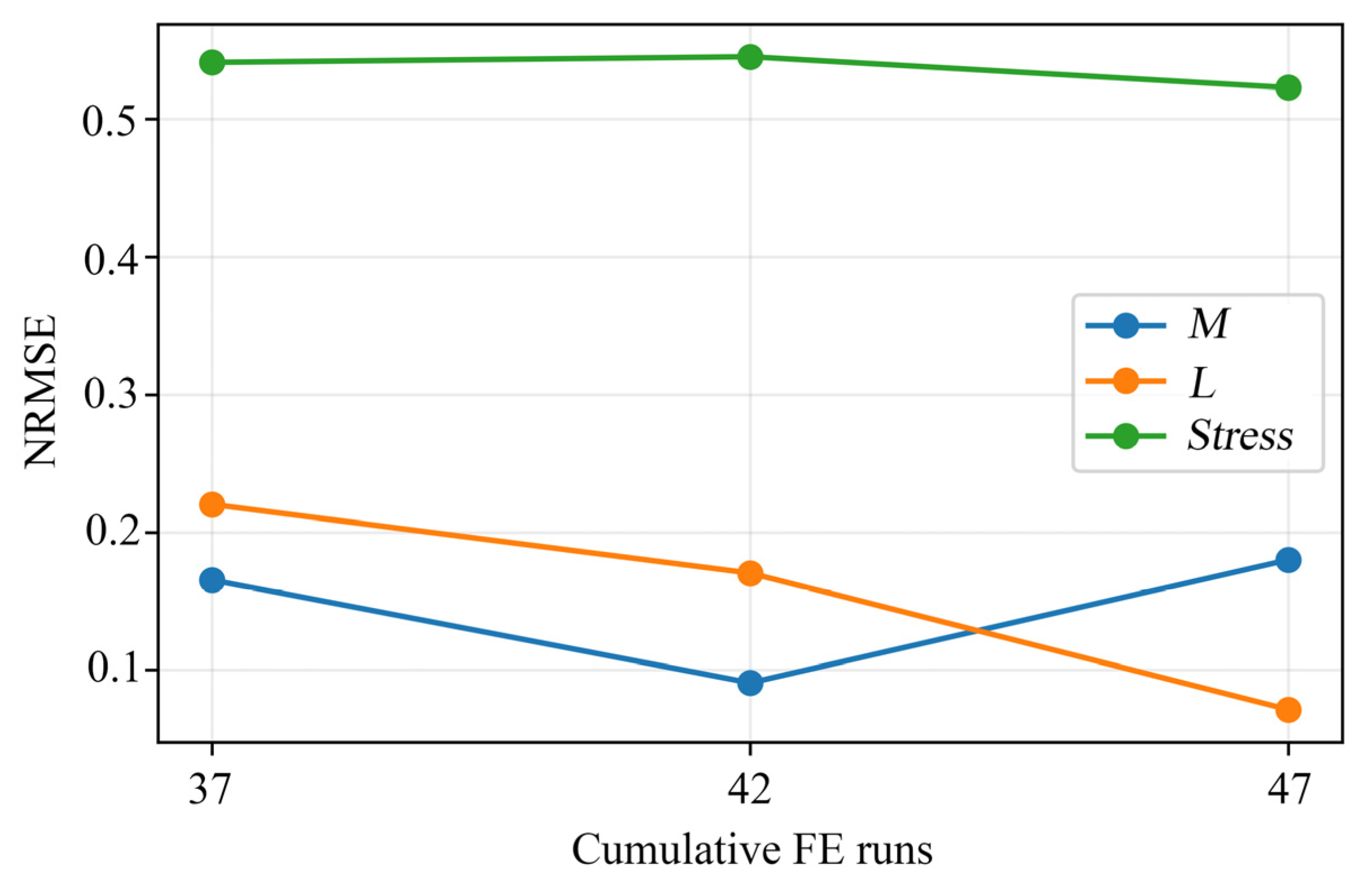
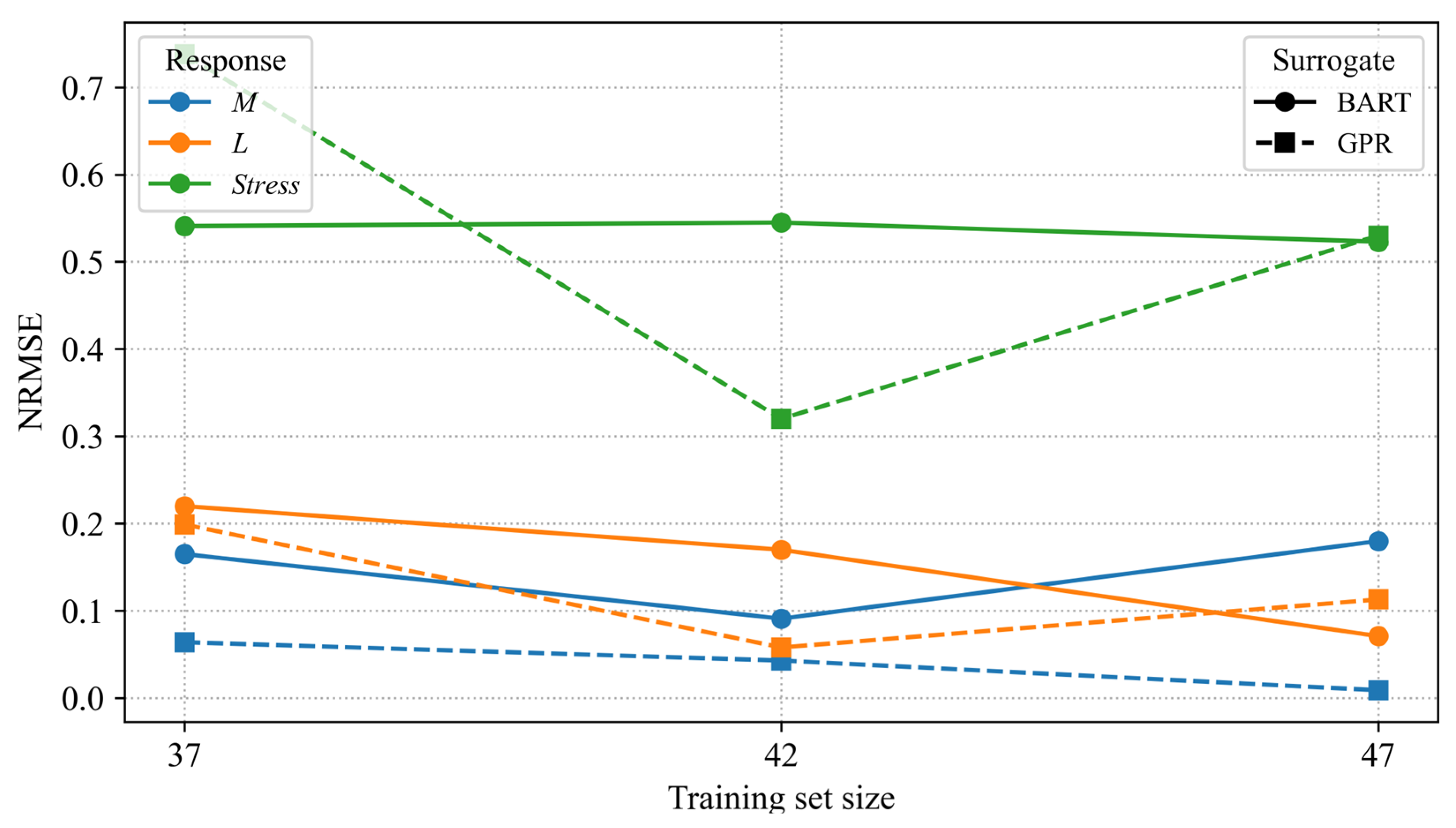
Figure 3 plots NRMSE against the cumulative training size, which grows from 37 to 42 and then 47 runs. Because each point is tested on a different upcoming batch, the curve reflects a prequential replay pattern rather than a conventional learning curve based on a fixed test set, so a strictly monotonic trend is not expected. In the results, L benefits noticeably from the added training data. The error for M stays low, with small fluctuations that likely arise from varying batch difficulty and the limited number of test samples. By contrast, Stress maintains a higher error level across stages, suggesting that peak stress is harder to model with the same amount of data. This is in line with the highly localized and contact-sensitive character of stress responses.
In this work, the sequential workflow is bounded by a fixed FE budget represented by the completed 50-run DOE dataset, and cost is expressed in FE-run units. The model is initialized with 37 runs, and enrichment is capped at 10 additional runs added in two batches of 5. The remaining 3 runs are reserved as a hold-out subset for final validation and are excluded from fitting, tuning, and any intermediate choices. The default stopping rule is to terminate once the enrichment budget is used. Early stopping may also be applied if the prequential test error shows no meaningful change over successive rounds.

2.6. Surrogate Modeling and Feasibility-Guided Enrichment

2.6.1. BART Surrogate (Primary)

Let x R d denote the design vector formed by the DOE variables in Table 1 (fixed quantities are not included). Separate surrogates are trained for the three scalar responses M, L, and Stress.
BART is used as the primary surrogate because it can capture strong nonlinearity and interaction effects with limited samples, while producing a posterior predictive distribution that supports uncertainty-aware analysis [27].
For each response y ∈ {M, L, Stress}, the regression function is represented as follows as a sum of m shallow trees:
y x = j = 1 m g x ; T j , Θ j + ε
where Tj and Θj are the structure and terminal-node parameters of the j-th tree, and ε denotes the residual. Posterior inference follows the Bayesian backfitting procedure, described as follows, and yields posterior predictive draws:
y t x t = 1 T
U x = 1 T 1 t = 1 T y t x y ^ x 2
The predictive mean is computed from these draws, and the predictive uncertainty is summarized by either the posterior standard deviation or the width of a chosen credible interval. In what follows, the uncertainty measure is denoted by U(x) and is computed in the same manner for all replay rounds.

2.6.2. Probability of Feasibility (PoF) Estimation

Because peak stress is both decision-critical and challenging to predict accurately under a limited explicit-FE budget, feasibility is evaluated from the posterior predictive distribution of Stress rather than from a single mean prediction. For a candidate design x, let S t r e s s S x s = 1 S denote the posterior predictive draws produced by the BART surrogate, where S is the number of draws (i.e., pred_draws). Given an engineering stress cap σlim, the feasibility probability is approximated via Monte Carlo counting:
P o F S t r e s s x = 1 S s = 1 S II S t r e s s s x σ l i m
No Gaussian or normal approximation is imposed. Designs satisfying PoFStress(x) ≥ η, with η = 0.90, are treated as feasible for enrichment ranking and for subsequent Pareto exploration. The threshold η = 0.90 is selected as a pragmatic balance between false rejection and false acceptance under a limited explicit-FE budget. A higher η lowers the chance of accepting borderline, stress-critical designs. However, it can also discard promising lightweight candidates when the stress surrogate remains uncertain. In contrast, a lower η increases exploration and coverage, but it admits more near-boundary designs.
Accordingly, η = 0.90 is used for enrichment ranking and feasible-Pareto exploration. Final recommendations are not accepted based on PoF alone. They are verified by independent high-fidelity FE reruns. For stress-critical design sign-off, a stricter gate (e.g., η = 0.95) is recommended.
A packaging-clearance constraint, L ≤ 20 mm, is applied as an additional post-screening rule. Under the adopted 100 kN termination rule, most DOE and candidate designs satisfy L(x) ≤ 20 mm with ample margin; therefore, this clearance screen is seldom active in the present dataset. It is retained as an explicit engineering constraint and may become controlling under larger pole travel, alternative termination criteria, or different packaging layouts.

2.6.3. Acquisition and Batch Enrichment

Candidates are ranked using a feasibility-weighted acquisition score, described as follows, where feasibility is quantified by PoFStress(x) and U(x) denotes predictive uncertainty:
A x = P o F S t r e s s x U x
where U(x) measures predictive uncertainty. When multiple responses are considered, U(x) is constructed as a weighted sum of normalized predictive standard deviations, described as follows:
U x = r M , L , S t r e s s ω r σ ¯ r x
With σ ¯ r x denoting the response-wise standard deviation after normalization by its scale and ωr denoting user-defined weights.
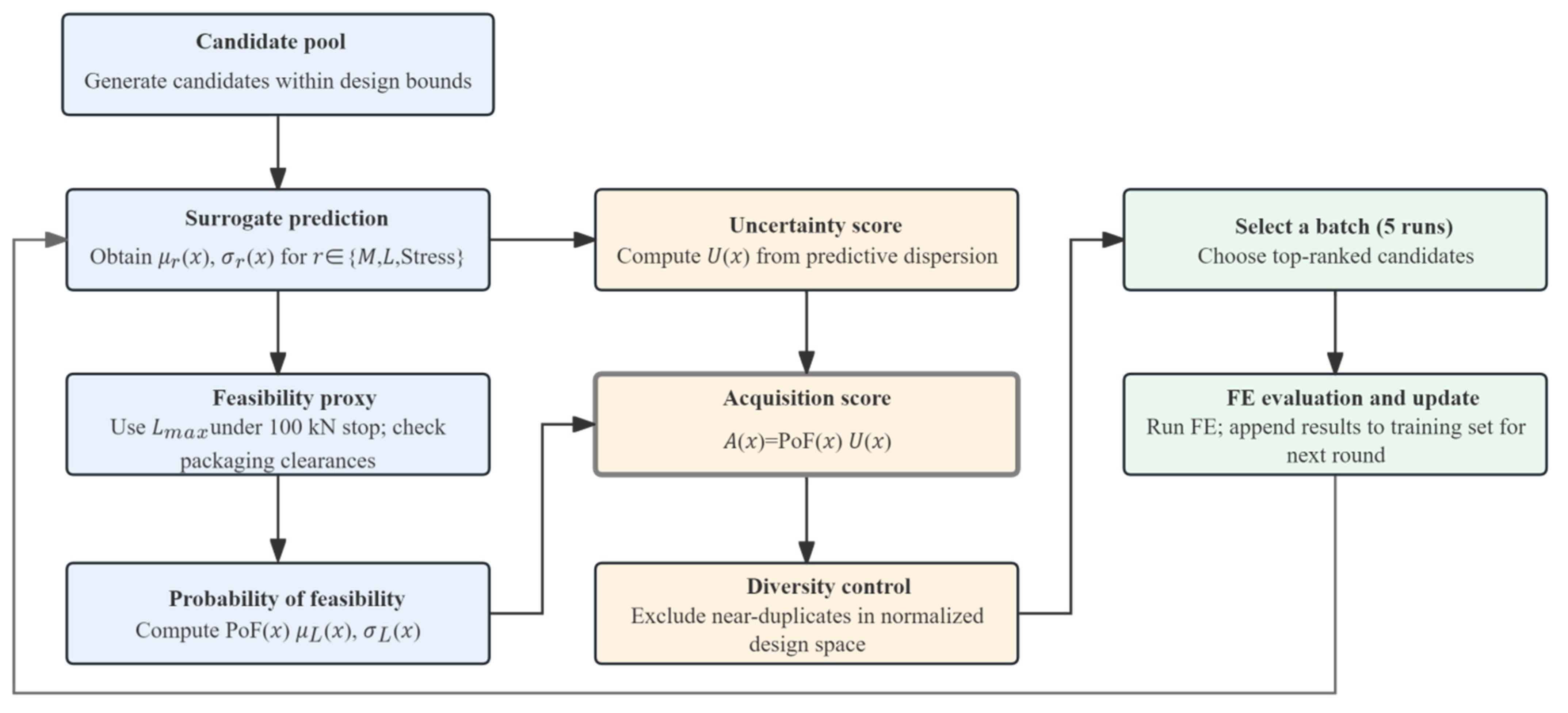
Batch construction follows the ranking while avoiding redundant points. After selecting a candidate, nearby candidates in the normalized design space are temporarily excluded so that the batch maintains diversity. The batch size matches the sequential plan used in the replay, with 5 runs added per round.
The feasibility-guided enrichment procedure is summarized in Figure 4.
Figure 4 illustrates the feasibility-guided enrichment logic adopted in the retrospective replay. Starting from the initial training set, a candidate pool is evaluated using the surrogate models. For each candidate x, BART yields posterior predictive samples for each response, from which the predictive mean and dispersion are estimated. Stress acceptability is measured using the probability of feasibility PoFStress(x), estimated from BART posterior predictive draws as defined in Section 2.6.2. Candidate ranking combines feasibility confidence, such as PoFStress(x) ≥ η with η = 0.90, and an uncertainty-driven exploration term.

2.6.4. GPR Reference and Model-Dependence Check

To mitigate model dependence, an additional Gaussian process regression (GPR/Kriging) surrogate is fitted for each response using the same data split and replay protocol. The GPR models act as an independent cross-check to verify that the main conclusions are not unduly driven by the choice of surrogate family [16,17,26,28]. In GPR, the response is modeled as a Gaussian process, described as follows:
y x ~ G P μ x ,   k x , x
where k(·,·) is the covariance kernel (with automatic relevance determination when applicable). Hyperparameters are estimated by maximizing the marginal likelihood on the training subset of the corresponding replay round. The fitted GPR yields closed-form predictions μ(x) and σ(x), which are used as a reference when comparing uncertainty estimates and downstream decisions against those obtained with BART.
Workflow from the 50-run DOE split (37/5/5/3) to surrogate training (BART with GPR check) and downstream use in retrospective replay and feasibility-guided enrichment.
The overall workflow and the roles of the two surrogate models are summarized in Figure 5.
To ensure that the conclusions drawn from the sequential study are not tied to a single surrogate type, a dependence check is conducted by repeating the analysis with a Gaussian process regression model. The intention is to use GPR as a transparent reference and to confirm that the observed error trends and the relative difficulty of predicting different responses remain consistent.
For each response, namely M, L, and Stress, a separate GPR surrogate is trained using the same input variables as in the BART runs. The 37/5/5/3 partition is kept unchanged. A Matérn kernel with ν = 2.5 is adopted with automatic relevance determination so that different length scales can be learned for different design variables. Hyperparameters are identified by maximizing the log marginal likelihood using only the available training subset at each stage. The fitted model then provides a predictive mean for point prediction and a predictive standard deviation as an uncertainty measure.
The GPR surrogate is evaluated using the identical test-then-update protocol described in Section 2.5.3. In Round 0, training uses the initial 37 runs and testing is performed on the first 5-run batch. In Round 1, the training set is expanded to 42 runs and testing is performed on the second 5-run batch. Finally, the model trained on 47 runs is assessed on the 3-run hold-out subset, which remains excluded from fitting and any intermediate choices throughout.
For each stage and each response, prediction performance is reported using RMSE, NRMSE, and R2, matching the metrics used for BART. The side-by-side comparison is summarized in Table 4 and serves as a consistency check for the learning behavior discussed earlier.
The comparison supports the main observation that L is learned more reliably than Stress under the same data regime, while Stress remains challenging due to its contact-sensitive nature.
Figure 6 provides a visual consistency check by plotting the prequential NRMSE trajectories of BART and GPR across the three stages.
Figure 6 indicates that the two surrogate models follow similar learning trends across the replay stages. As more runs are added, the prediction error for L generally decreases, whereas Stress remains more challenging to capture within the same sampling budget. Small non-monotonic fluctuations are expected, since each stage is tested on a different “next” batch rather than on a single fixed validation set.
Since the enrichment step in Section 2.6.3 relies on a feasibility-weighted uncertainty ranking, a supplementary check can be performed at the ranking level. Using the same candidate pool, acquisition scores produced by BART and by GPR are ranked and compared. Agreement is quantified using Kendall’s τ. This check evaluates robustness of the selection logic without introducing additional FE evaluations.

2.7. Optimization and Decision Pipeline

2.7.1. NSGA-II Configuration and Constraint Handling

Multi-objective optimization is performed exclusively for the −40 °C side-pole rigid-pole extrusion scenario. Both objective evaluation and feasibility screening are provided by the final surrogate models developed in Section 2.5.3, trained on n = 47 high-fidelity samples. Their predictive performance is summarized in Table 4, and the corresponding prequential behavior is shown in Figure 6; together, these results serve as the error reference for the optimization stage. To emphasize the surrogate-assisted workflow rather than optimizer selection, NSGA-II is used as a standard evolutionary multi-objective baseline to generate a diverse approximation of the Pareto set, in line with typical practice in crashworthiness-driven structural optimization and battery protection design [29,30,31].
The design vector is x = [x1, …, x9], where x1x5 are thickness variables and x6x9 are discrete layup weights that are normalized into ply ratios. Variable bounds and admissible levels follow the parametric FE model and are listed in Table 1. Two objectives are minimized simultaneously: the enclosure mass M (x) and the peak displacement L (x). Mechanical acceptability is enforced through a stress-based feasibility requirement implemented in probabilistic form.
NSGA-II variation operators (SBX crossover and polynomial mutation) are applied in the continuous decision space. After variation, the discrete thickness variables (x4 and x5) are projected to the nearest admissible DOE level. The layup-weight variables (x6x9) are first normalized into ply ratios and then converted into a manufacturable integer ply schedule using the same rounding-and-repair procedure described in Section 2.2, including enforcement of balanced ±45° plies. This projection/repair step is applied to every offspring before surrogate evaluation.
NSGA-II is run with Npop = 200 and Ngen = 400, using SBX (pc = 0.9, ηc = 20) and polynomial mutation (pm = 1/9, ηm = 20), with a fixed base seed of 2025. All solver settings are kept constant across runs and are summarized in Table 5.

2.7.2. Screening + TOPSIS

The feasible Pareto set contains many alternatives with nearly indistinguishable trade-offs, so selecting a single “best” design directly is neither transparent nor efficient for verification planning. A two-step procedure was therefore adopted.
First, a compact candidate subset was extracted by interval-based filtering within each Pareto branch. Specifically, solutions in each branch were stratified into equal-mass bins, and six solutions were retained per branch (K = 12 in total). This sampling strategy preserves diversity and branch representativeness while avoiding redundant points clustered in a narrow region of the front.
Second, TOPSIS was applied to the candidate subset using mass M and peak displacement L as cost-type criteria with equal weights (ωM = ωL = 0.5) [32]. This yields a closeness score and a ranked list, from which the highest-ranked candidate was taken as the representative design for engineering interpretation of the feasible trade-off set. Independent validation is then carried out in Section 3 using the hold-out runs that were kept entirely separate from surrogate training.

2.7.3. Candidate Selection for FE Reruns

To close the surrogate-to-FE decision loop, a two-candidate rerun protocol was defined. It included (i) one representative design selected by TOPSIS from the feasible Pareto set and (ii) one near-threshold design with PoF close to the adopted cutoff (~0.90) to test robustness at the feasibility boundary. An optional high-margin reference design (PoF ~0.95) was also considered. The final candidate IDs and FE rerun results are reported in Section 3.4.

2.8. Implementation Details and Reproducibility

Traceable results are emphasized under a limited simulation budget. All responses are obtained from 50 high-fidelity FE runs, which provide mass M, peak displacement L, and peak stress (Stress). These FE outputs are treated as the only ground truth used in the subsequent surrogate and selection steps.
A combined workflow is adopted to link FE evaluation with surrogate-assisted analysis. The FE model generates the response database under the side-pole rigid-pole extrusion condition. Two surrogate families are considered. BART is implemented in Python 3.12 (PyMC 5.27.0 with PyMC-BART 0.11.0) and serves as the primary model, because it offers both nonlinear regression capability and posterior predictive uncertainty required by the selection rule. GPR is implemented in Python and is used as an auxiliary baseline to perform a surrogate-dependence check, ensuring that the main observations are not driven by a single modeling choice. PyMC uses the PyTensor automatic-differentiation backend to support gradient-based samplers (e.g., NUTS) for continuous parameters. In this study, all variables and responses are real-valued. Therefore, only standard real-valued gradients are needed, and no complex-valued differentiation is involved.
The full DOE budget is fixed at 50 FE runs. Within this dataset, only 10 runs are regarded as the sequentially deployable budget and are introduced in two rounds (5 + 5). The remaining 3 runs form a hold-out set reserved for independent evaluation and are excluded from training and selection throughout. Accordingly, the data are partitioned into a 37/5/5/3 split and assessed by retrospective replay:
Stage 1: train on 37 runs and evaluate on the next batch of 5 runs;
Stage 2: train on 42 runs (37 + 5) and evaluate on the next batch of 5 runs;
Stage 3: train on 47 runs (37 + 5 + 5) and evaluate on the hold-out 3 runs.
This setup supports the learning-curve evidence (A) under a fixed budget while maintaining an untouched subset for an independent check.
At each stage, input scaling is performed using statistics computed from the current training subset only, avoiding any leakage from later batches. The replay partition is stored explicitly as a run-ID split file, and fixed random seeds are used for BART sampling and any stochastic components. Stage-specific seeds are generated deterministically from a base seed and the corresponding training size, so that repeated runs follow the same replay trajectory.
In the sequential module, Stress is treated as a feasibility constraint. Candidate ranking follows a feasibility-aware criterion of the form PoF × uncertainty (B), prioritizing points that are likely feasible while still informative for model improvement. For transparency and downstream visualization, the workflow exports stage-wise error summaries (RMSE/NRMSE/R2), per-point predictions with uncertainty, learning-curve figures, and PoF/score diagnostic plots used for ranking.
The key settings that determine reproducibility are summarized in Table 6.
Overall, this section establishes a traceable surrogate-assisted workflow under a fixed budget of 50 FE runs. Surrogate behavior is assessed via a prequential replay to track accuracy changes as additional data are introduced, while feasibility-guided enrichment targets decision-relevant regions using a PoF-weighted uncertainty criterion with Stress treated as the constraint. Post-training efficiency is quantified through a reproducible benchmark using stored posterior samples. Inference is performed via posterior predictive evaluation only (sans MCMC sampling), separating the one-time overhead (graph reconstruction) from the steady-state latency. Results confirm that surrogate evaluation is orders of magnitude faster than the explicit FE solver. The posterior predictive draw count matches Table 6, and repeated trials are used to summarize median and p95 statistics. The timing results and the FE-to-surrogate acceleration ledger are summarized in Section 3.5.

3. Results

3.1. Hold-Out Validation of Surrogates

The 50-run DOE is organized into four parts: 37 initial runs, two enrichment stages of 5 runs each, and a final hold-out set of 3 runs reserved exclusively for independent validation. The hold-out data are kept completely separate from surrogate fitting and any model-selection decisions, and are used only for independent validation of the final surrogate.
The hold-out results indicate that the peak displacement L is predicted with high accuracy, with relative deviations around one percent across all three cases. By comparison, Stress shows substantially larger errors, reaching roughly twenty percent for one case. Such behavior is consistent with a contact-dominated quantity that depends strongly on localized deformation, stress concentration, and small variations in contact evolution.
These findings support role separation within the workflow. The displacement surrogate is sufficiently accurate to serve as the objective evaluator for mapping the mass–intrusion compromise, whereas Stress is not suited to be enforced as a deterministic point constraint. Instead, stress acceptability is handled through an uncertainty-aware feasibility criterion.

3.2. Feasible Pareto Set and Trade-Offs

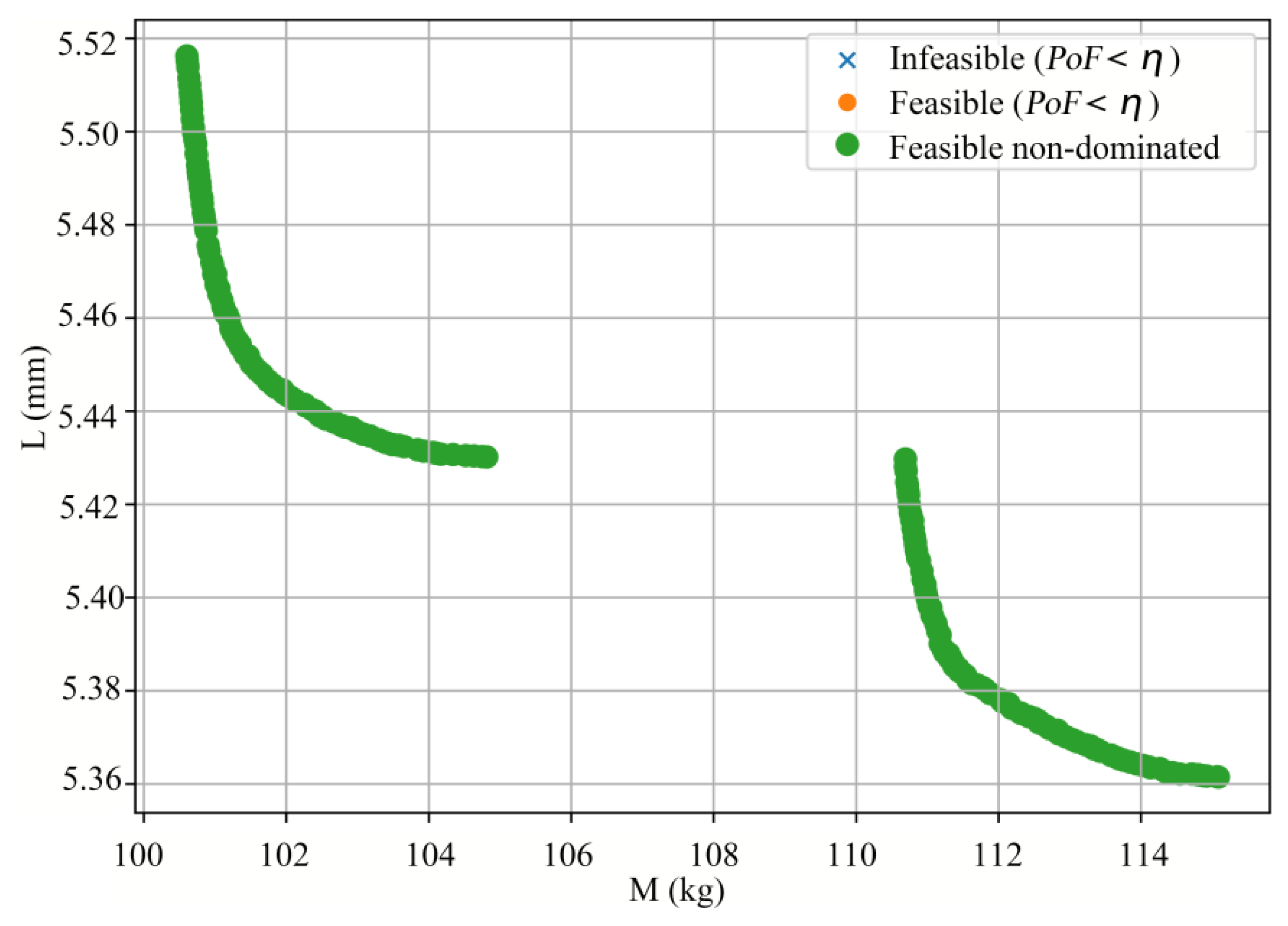
Figure 7 shows the obtained mass–displacement trade-off at −40 °C under the probabilistic stress constraint, where feasibility is defined by PoFStress(x) ≥ η (η = 0.90). As expected, reducing mass generally increases the peak displacement, while tighter displacement control requires additional material. The PoF filter is most influential in the low-mass region, where stress margins are narrow and uncertainty becomes non-negligible; therefore, designs that look attractive under mean predictions may still be rejected when feasibility confidence is enforced. The feasible set in Figure 7 is thus treated as an engineering-relevant candidate pool for subsequent selection and verification, rather than a purely mathematical Pareto boundary.
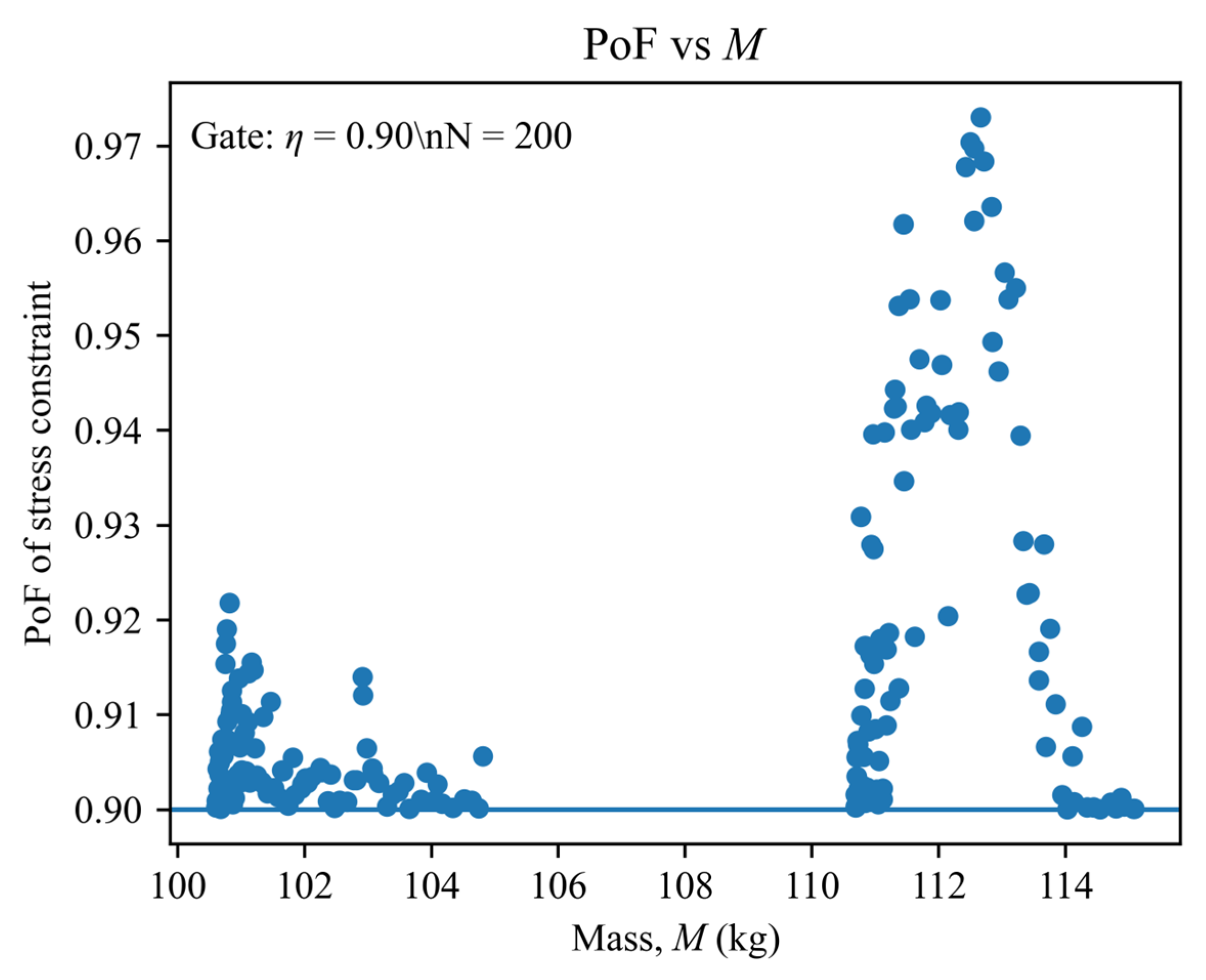
Appendix A, Figure A1 illustrates the distribution of PoFStress across the feasible Pareto pool and marks the adopted screening threshold, η = 0.90.
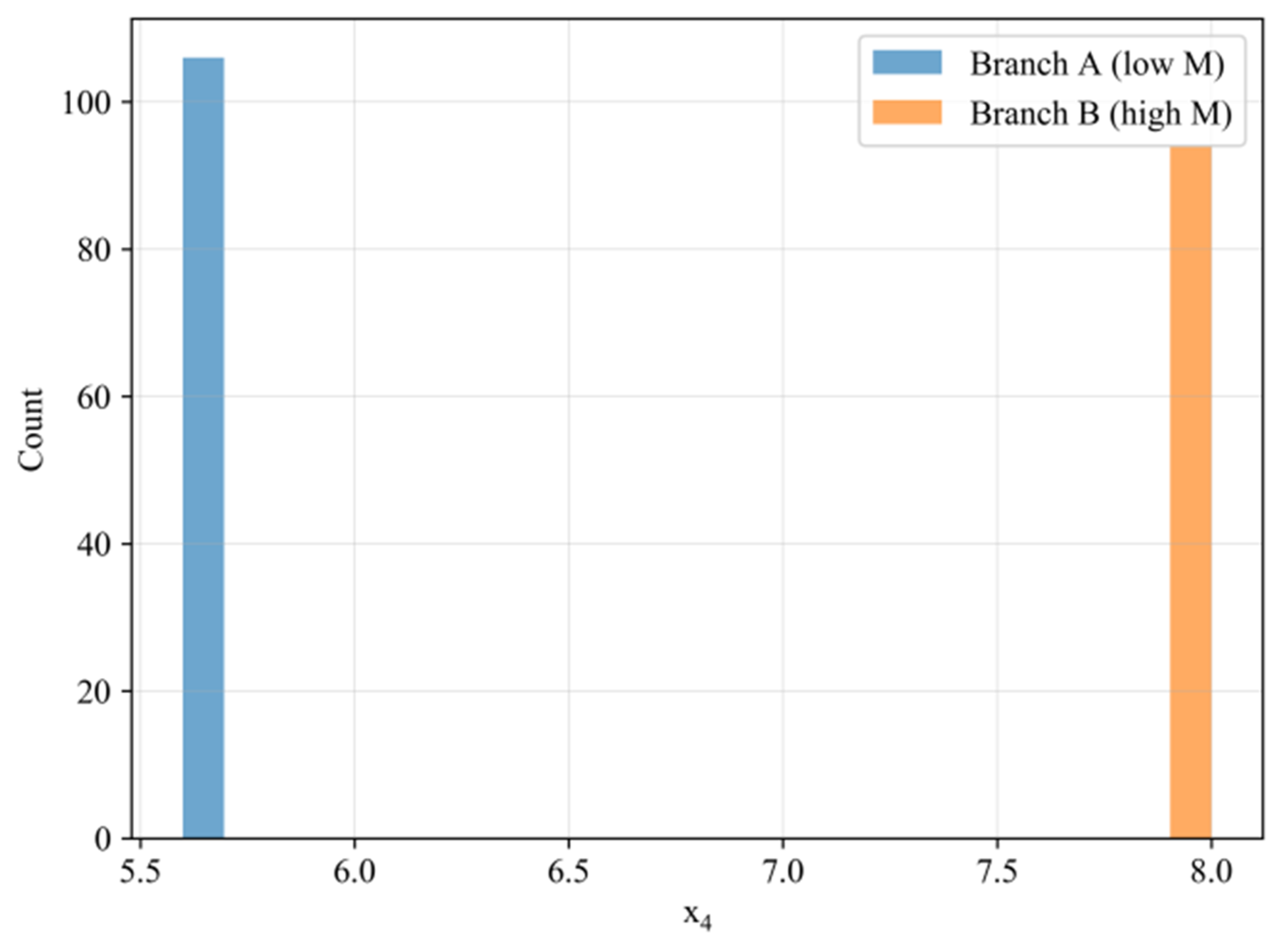
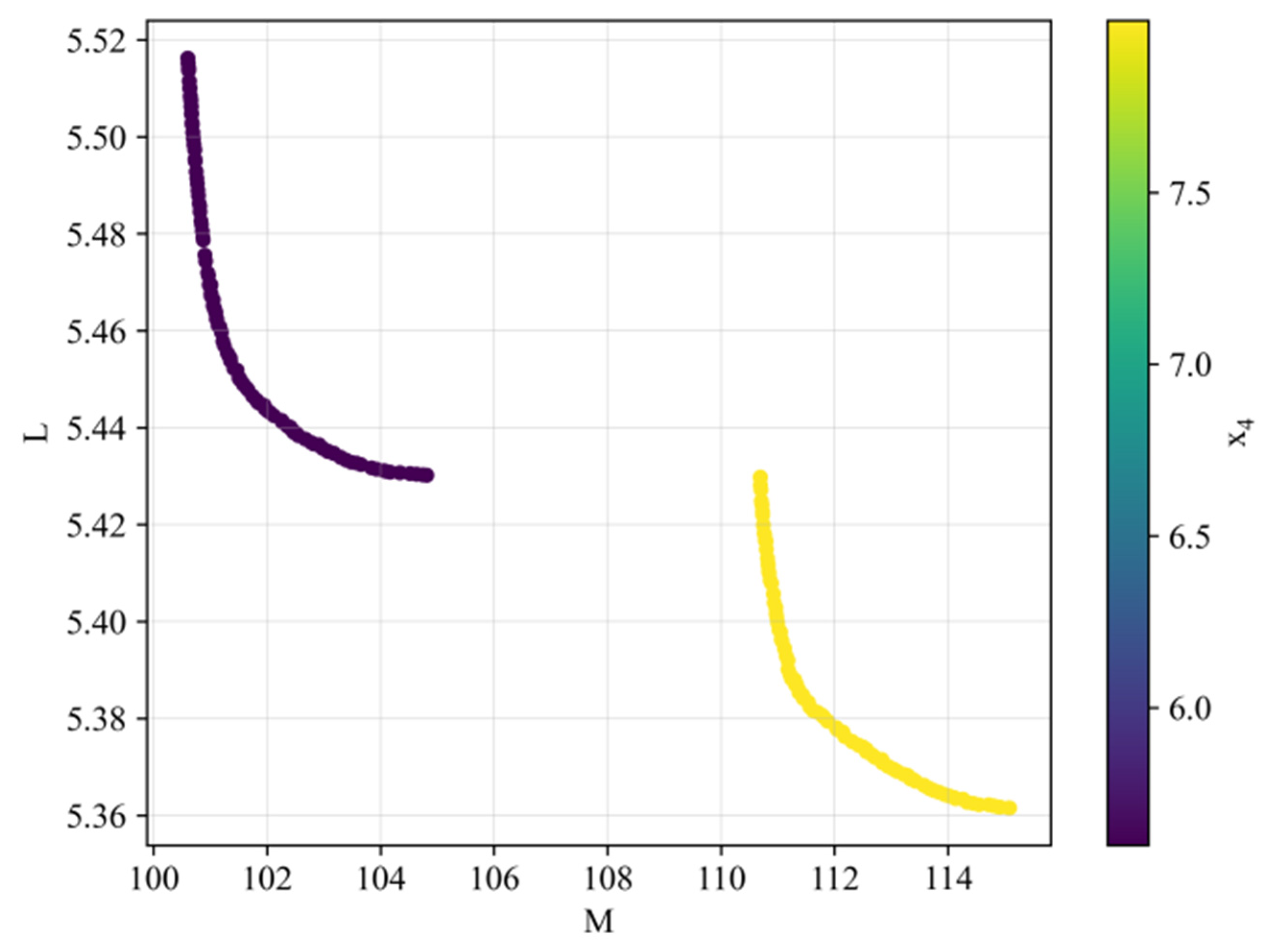
A notable feature is that the feasible non-dominated set appears as two separate segments. This split is clarified in Figure 8: the two segments correspond to two distinct levels of the key thickness variable x4, indicating two competing design regimes. In the current dataset, x4 exhibits a bimodal distribution (Figure A2), and the branch statistics are summarized in Table 7. For PoF, Table 7 lists the branch-wise range and the corresponding dispersion (sample standard deviation) over the non-dominated solutions. Practically, increasing x4 shifts the response to a stiffer deformation pattern, leading to a lower displacement at the expense of higher mass, while the PoF constraint removes part of the intermediate region where feasibility confidence does not meet η. The full branch statistics, including the predicted mean and uncertainty of stress, are provided in Supplementary Material (Table S2).
Although both branches follow the same −40 °C rigid-pole extrusion setup and termination rule, they represent two stiffness-controlled deformation regimes governed primarily by the lower-case thickness x4. Branch I (lower mass, thinner x4) is more compliant in out-of-plane bending. It promotes a more global deformation of the enclosure floor–side assembly and spreads the pole-induced load over a broader load path. This regime therefore behaves like a global-compliance response: intrusion reduction is achieved mainly by increasing overall structural stiffness rather than by tuning local contact stiffness.
Branch II (lower L, thicker x4) increases local bending stiffness and constraint near the pole–contact region. It tends to suppress local instability and section ovalization, and it shifts the response toward a more localized indentation mode. Load transfer is redirected more effectively into adjacent stiff members (e.g., side rails and cross members) along the load path. This yields slightly lower intrusion at the cost of higher mass, and it can also increase sensitivity to contact-driven stress peaks.
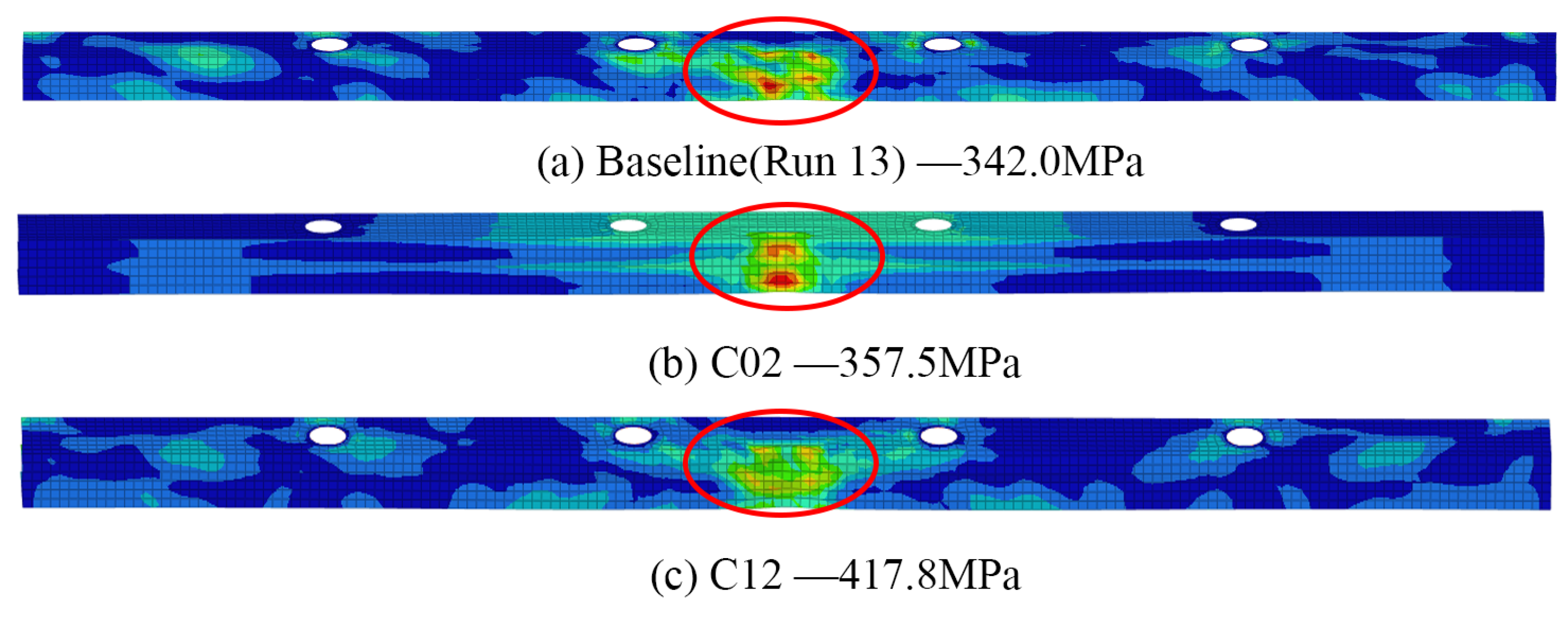
Feasibility is therefore governed by a localized peak response, even when the overall displacement pattern is broadly similar across designs (Figure 9). This local–global contrast is consistent with the FE reruns: stress concentrations remain confined to the pole-contact zone of the lateral anti-collision beam (Figure 10).
Feasibility is screened using the probabilistic stress gate defined in Section 2.6.2 (η = 0.90) together with an intrusion-based packaging-clearance check. This screening step filters out designs that achieve lower intrusion only by inducing excessive stress concentration on the lateral anti-collision beam, thereby yielding a more defensible feasible Pareto set for downstream selection. Notably, the retained solutions become sparse near the extreme low-mass end, implying that stress compliance is the primary limiting factor in that region.

3.3. Candidate Screening and TOPSIS Selection

To reduce sensitivity to a single surrogate formulation, the same candidate subset was re-evaluated using PI-GPR, and the TOPSIS ranking was recomputed. Agreement between the two rankings was quantified by Kendall’s τ (τ = 0.606 in this study), indicating moderate ranking consistency. Candidate information and the TOPSIS outcomes before and after the re-evaluation are summarized in Table 8. In this study, C02 from Branch I is adopted as the representative design produced by the decision procedure. The final surrogates are first validated on the reserved hold-out set, followed by additional FE reruns for selected surrogate-recommended candidates (C02 and C12, with C09 included as an optional high-margin case) [33]. The full candidate information is provided as Supplementary Table S3.
Because many feasible Pareto solutions are practically indistinguishable, the set is reduced to a compact candidate pool using interval-based filtering applied separately within each Pareto branch. Six candidates are retained per branch, giving K = 12. TOPSIS is then performed on this screened subset, using (M, L) as cost-type criteria with equal weights, ωM = ωL = 0.5.
To reduce sensitivity to a single surrogate family, the same candidates are re-evaluated with PI-GPR and the TOPSIS ranking is recomputed. The agreement between the two rankings, quantified by Kendall’s τ = 0.606, indicates moderate stability with limited swapping among the leading candidates. Under this decision chain, design C02 from Branch I is selected as the representative solution for subsequent interpretation.

3.4. High-Fidelity FE Reruns and Acceptance Outcomes

Table 9 presents the independent validation results for the hold-out set with n = 3, where surrogate estimates are benchmarked against the corresponding high-fidelity FE outputs. For each response y ∈ {M, L, Stress}, the absolute and relative deviations are defined as
Δ y = y F E y s u r
Table 9 indicates that the surrogate reproduces the peak displacement L on the hold-out runs with good accuracy, with relative deviations on the order of 1% for all three cases. For mass M, a small systematic offset is observed on this subset. The two heavier hold-out designs are slightly underestimated by about 4%, whereas the remaining case is overestimated by about 2%, giving an average absolute relative deviation of approximately 3–4%. This discrepancy is acceptable for the present analysis because M is retained mainly to keep the surrogate workflow consistent with the DOE-based learning procedure. In engineering use, mass can be obtained deterministically from the geometry and material density once the design variables are fixed.
The stress response exhibits larger deviations, which is consistent with its contact-driven nature and its sensitivity to local deformation patterns, stress concentrations, and minor changes in contact evolution. Taken together, the hold-out benchmark provides an unbiased assessment of generalization and supports using the final surrogates as the evaluation engine for feasibility-aware optimization and candidate screening in subsequent analyses.
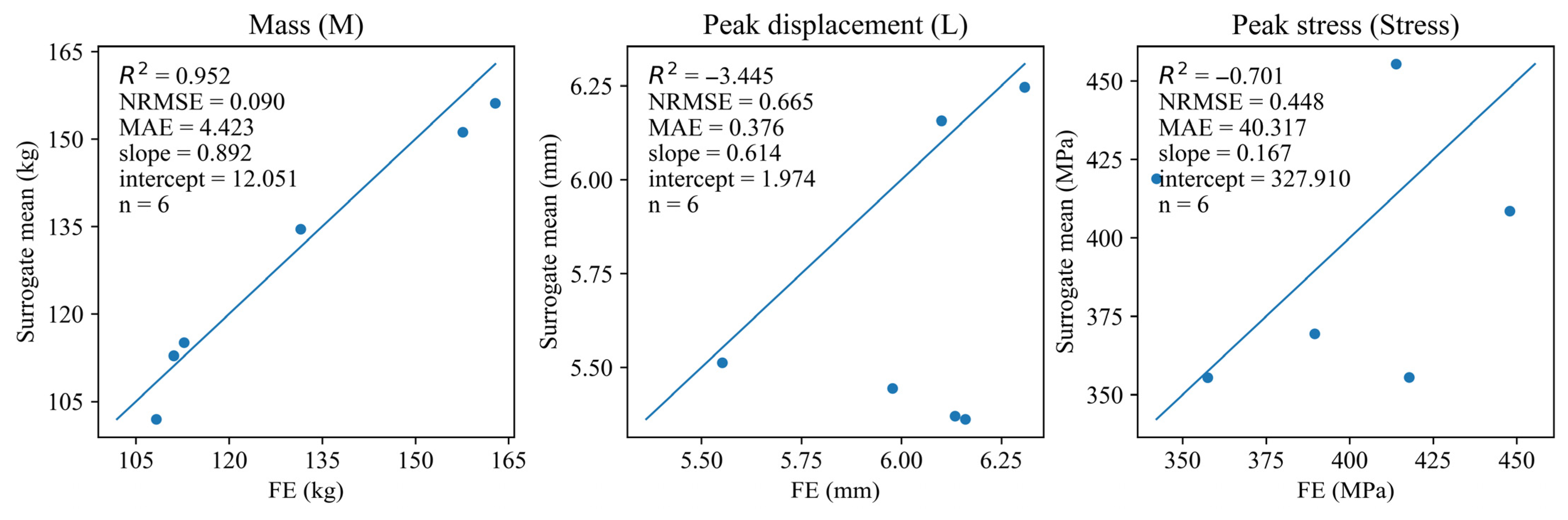
To complement the tabulated error metrics, Figure A3 presents parity plots comparing the surrogate posterior mean with the FE results for both the hold-out cases and the rerun candidates. The peak displacement predictions closely follow the 1:1 line, whereas the stress response exhibits a visibly broader spread. This contrast motivates the use of a probabilistic feasibility screen in the subsequent selection to mitigate the risk of choosing designs near the stress limit.
Following the protocol in Section 2.7.3, two surrogate-selected candidates were prioritized for independent high-fidelity FE reruns. C02 (Branch I) was chosen as the TOPSIS representative from the feasible Pareto set. C12 (Branch II) was chosen as a near-threshold case (PoF ≈ 0.90) to assess the conservativeness of the PoF gate and the risk of borderline misclassification. A higher-margin Branch II design, C09 (PoF ≈ 0.95), was retained as an optional within-branch reference.
The reruns strictly follow the FE setup specified earlier, including geometry, boundary conditions, contact formulation, −40 °C material properties, and the response extraction procedure; these details are not repeated here. For each candidate, the same termination rule is applied (simulation is terminated when the reaction force reaches 100 kN or the prescribed travel reaches 30%, whichever occurs first). The mass M, peak intrusion L, and peak stress (Stress) are extracted using the same definitions adopted in the DOE simulations.
For surrogate reporting, Msur and Lsur correspond to the posterior predictive means from the final BART models, while Stresssur is reported as the posterior mean. The feasibility probability PoFStress(x) is computed by Monte Carlo counting over BART posterior predictive draws as defined in Section 2.6.2.
Table 10 summarizes the surrogate–FE comparison for three surrogate-selected candidates, C02, C09, and C12, under the −40 °C side-pole rigid-pole extrusion scenario. For each response y∈{M, L, Stress}, the relative deviation is computed in the same way as in the hold-out benchmark (Table 9), described as follows:
δ y % = y s u r y F E y F E × 100
These reruns are decision-oriented rather than purely diagnostic. They directly verify the designs recommended by surrogate-assisted optimization and quantify the risk associated with stress prediction, particularly for candidates close to the feasibility threshold.
To ensure comparability, all FE reruns replicate the DOE setup, including geometry definition, boundary conditions, contact parameters, −40 °C material properties, and response extraction rules. Mass is reported for the battery-pack enclosure only, excluding the rigid pole and fixtures, consistent with the DOE dataset used for surrogate training and optimization.
Table 10 demonstrates a high degree of concordance between the predicted mass and the FE validation results, with relative errors (δM) confined within approximately ±6% across the three candidates. In contrast, the peak displacement (L) is consistently underpredicted (δL ranging from −9% to −13%), suggesting that the surrogate model yields slightly optimistic displacement estimates within this local design space. Notwithstanding this systematic bias, the performance trends remain coherent: Branch II candidates are predicted to have a smaller $L$, while FE reruns confirm comparable intrusion levels between the two Branch II points. Regarding stress constraints, candidates C02 and C09 remained within admissible limits during high-fidelity validation. Conversely, C12 exceeded the threshold (StressFE = 417.8 MPa), despite possessing a Probability of Feasibility (PoF ≈ 0.90) that satisfied the initial screening criterion. This observation also highlights threshold sensitivity. Using η = 0.90 can admit near-boundary candidates such as C12 (PoF ≈ 0.90) that still carry residual failure risk under highly localized contact stresses. This discrepancy highlights a critical insight: candidates situated near the feasibility boundary entail a residual risk of failure, exacerbated by the highly localized nature of contact stress. The violation in C12 underscores the imperative of a probabilistic framework; a deterministic surrogate, by neglecting predictive variance, would have obscured such borderline risks. Consequently, for stress-critical components in battery safety engineering, adopting a more stringent PoF threshold (e.g., η = 0.95) is warranted to ensure structural integrity. In contrast, a stricter gate such as η = 0.95 would favor higher-margin designs (e.g., C09 with PoF ≈ 0.95). This reduces false acceptance, but it may also exclude borderline lightweight candidates.
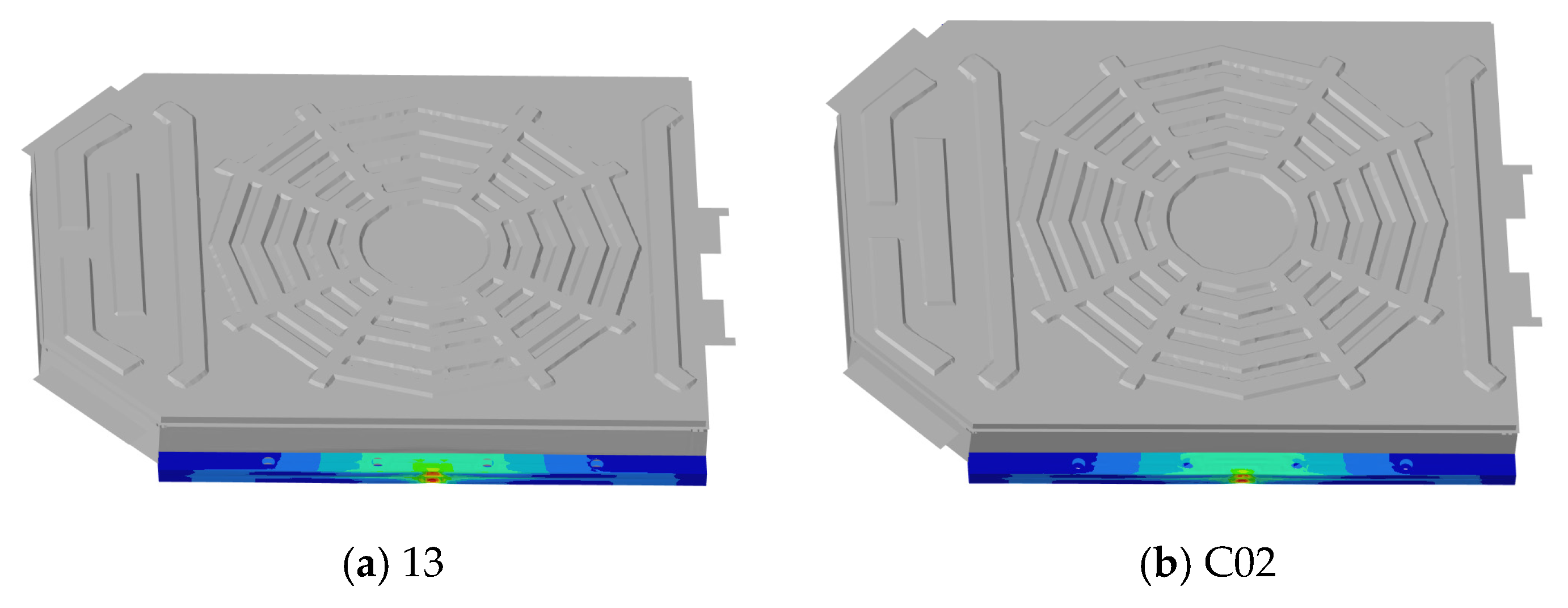
Figure 9 juxtaposes the −40 °C displacement fields of the baseline (Run 13) and C02 at the 100 kN cut-off, to confirm that the surrogate-selected design maintains the same deformation mechanism while mitigating intrusion.
Relative to the baseline, C02 achieves a smaller peak intrusion while exhibiting a comparable global deformation pattern. This visual evidence agrees with the reduced peak displacement L reported in Table 10.
As illustrated in Figure 10, stress concentrations are confined to the pole-contact zone of the lateral anti-collision beam, suggesting that feasibility is dictated by a local peak response rather than the overall deformation pattern. In the FE reruns, C02 attains a maximum stress of 357.5 MPa, which satisfies the limit σlim = 410.4 MPa, whereas C12 rises to 417.8 MPa and exceeds the cap. These results motivate the probabilistic feasibility screening adopted in the surrogate-assisted optimization, helping avoid recommendations that lie too close to the stress boundary.
In addition to demonstrating numerical consistency, the FE reruns in Table 10 provide direct confirmation of the surrogate-selected candidates using the same response definitions adopted throughout this work. Final engineering sign-off is based on a transparent pass–fail scheme that couples a baseline-referenced stress cap with a packaging-clearance requirement. Stress compliance is judged against σlim as defined in Section 2.6.2; under this check, C02 and C09 satisfy the limit, whereas C12 exceeds it in the rerun.
The clearance criterion is also met for all three candidates, since the predicted intrusions remain at the millimeter level and are well within the available packaging gap.
Taken together, these checks create a consistent bridge from PoF-based screening to the deterministic acceptance decision from explicit FE, thereby supporting C02 as the final representative design while keeping C09 as a feasible Branch II reference.

3.5. Sample Economy and Acceleration Ledger

High-fidelity FE runs for the −40 °C side-pole case are time-consuming. With the adopted termination criterion, one FE evaluation takes about tFE ≈ 23 min on the workstation used in this study. After training, surrogate evaluation is sub-second: the median wall-clock time is 0.394 s per design (p95 0.595 s), and 0.160 s per design (p95 0.231 s) when averaged over batch scoring, including, PoFStress. Compared with tFE ≈ 23 min, this implies an evaluation-level acceleration of roughly 3.5 × 10³ (single-point median) to 8.6 × 10³ (batch-amortized median), with conservative p95-based bounds of 2.3 × 10³ to 6.0 × 10³.
During model setup, short pilot runs were performed to verify the termination response. Each pilot case was halted when the reaction force reached 100 kN, which in most instances occurred within the first six recorded output steps. These pilot runs took about 23 min to complete and are excluded from the acceleration ledger, as they were not treated as production-grade high-fidelity evaluations.
To clarify the stopping rule, Figure 11 presents the reaction force–intrusion histories of the baseline (Run 13) and the surrogate-selected rerun candidates (C02 and C12). The horizontal line denotes the 100 kN termination threshold, and the marker indicates the first output step at which the recorded force exceeds this limit.

4. Discussion

4.1. Implications for Feasibility Screening and Final Acceptance

Table 9 provides two observations that directly affect the surrogate-assisted decision process. First, the peak displacement L is reproduced consistently, indicating that the displacement surrogate is adequate for objective evaluation and for tracing the mass–intrusion compromise that forms the Pareto set in subsequent analyses. The second is that the stress response exhibits visibly larger deviations. This is not unexpected, as peak stress in a contact-dominated event is highly sensitive to local deformation modes, stress concentrations, and small differences in contact evolution. For this reason, a deterministic pass–fail rule based on a single stress point estimate would tend to admit borderline candidates that may exceed the limit once re-evaluated by explicit FE, and a probabilistic screen is preferred.
During optimization, feasibility is therefore imposed using the gate PoFStress(x) ≥ η with η = 0.90, so that the uncertainty of the stress surrogate is explicitly reflected in candidate screening. Final engineering acceptance, however, is determined deterministically from explicit FE outputs using the same response definitions and termination rule adopted in the DOE model. The stress requirement is checked against the baseline-referenced cap in Equation (8) (with the screening inequality in Equation (5), which gives σlim = 410.4 MPa (≈410 MPa). A packaging-clearance check is also applied by rejecting designs with excessive intrusion (L > 20 mm). Together, these checks yield a traceable pass–fail rule that is consistent with the adopted constraint-handling strategy and can be used directly when reporting the outcomes of subsequent FE reruns.
The runtime results distinguish one-time overhead (posterior loading and graph reconstruction) from the steady-state per-design inference cost. Since FE analyses in this study are terminated at the 100 kN criterion, the reference cost tFE reflects an early-terminated evaluation (≈23 min) rather than a full-length crash simulation. Although absolute timings vary with hardware and the number of posterior predictive draws, the settings used here keep inference in the sub-second range and support uncertainty-aware screening in routine use.

4.2. Applicability and Reproducibility Considerations

This section summarizes the outcomes of the surrogate-assisted workflow for the battery pack enclosure under the extreme-cold design condition T = −40 °C in the side-pole rigid-pole extrusion scenario.
All results reported here correspond to the discrete extreme-cold condition T = −40 °C under the adopted side-pole configuration, and no interpolation to other temperatures is assumed. Stress feasibility is enforced through PoFStress to reflect surrogate uncertainty and to limit the admission of borderline candidates. Reproducibility is supported by fixed data partitions with split indices 37/5/5/3, an explicit replay protocol, and a deterministic screening-to-TOPSIS procedure once the random seed is specified. The full DOE dataset, screened candidate lists, and ranking outputs should be provided as Supplementary Materials to enable auditability and reuse.

4.3. Limitations and Robustness

This study relies on high-fidelity FE simulations parameterized via literature-derived material properties, in the absence of component-level physical crash validation for the specific enclosure designs. While the proposed Bayesian framework effectively quantifies the uncertainty propagated from the surrogate model, it cannot entirely eliminate the epistemic uncertainty inherent in the baseline material inputs. Future work will address this by integrating experimental coupon data directly into the Bayesian prior to bridge the discrepancy between literature values and in situ material behavior. Furthermore, the violation observed in the C12 candidate underscores that while the PoF gate enhances reliability compared to deterministic approaches, ‘borderline feasible’ designs necessitate rigorous confirmatory verification. Future work will incorporate material variability directly in FE by using coupon-informed parameter sampling and a small number of material-perturbed replicate runs to calibrate response-level variability.
CFRP components are modeled using linear orthotropic elasticity, without progressive damage or delamination. This choice keeps the explicit-dynamics DOE traceable and computationally feasible under a limited FE budget. It also avoids additional model-form uncertainty from damage parameters that are difficult to calibrate at −40 °C, including intralaminar strengths, fracture energies, and cohesive interface properties for the adopted laminate and joints. Accordingly, the stress-based feasibility criterion used here should be interpreted as an elastic screening proxy, not as a definitive failure criterion.
If progressive damage were enabled (e.g., Hashin/Puck-type intralaminar criteria with stiffness degradation, together with cohesive-zone or continuum-damage formulations for delamination), three effects are expected. First, matrix-dominated damage may initiate earlier at low temperature. Feasibility defined by stress margin could then become more conservative when reformulated in terms of damage indices. Second, as damage accumulates, local stress hot-spots may be reduced by load redistribution, while stiffness degradation increases global compliance. As a result, intrusion L may increase for designs near the constraint boundary, meaning the elastic model can be slightly optimistic for borderline cases. Third, feasibility would be more appropriately expressed using damage-relevant metrics (e.g., peak failure index, damage variables, or delamination area/energy) rather than a single von Mises stress scalar. The same uncertainty-aware PoF framework can be applied to these metrics, but PoF values and ranking near the threshold are expected to change. This motivates confirmatory reruns for borderline designs, as illustrated by C12.
Despite this limitation, the observed two-regime Pareto structure governed by x4 is primarily driven by global load-path stiffness and contact kinematics. It is therefore expected to remain qualitatively stable. In contrast, stress-margin ranking and near-threshold feasibility may shift once damage is enabled, which we view as the logical next step toward design sign-off.
In addition, strain-based metrics and beam energy absorption provide practical alternatives to stress for characterizing crash response, and they can be screened using the same PoF framework once the corresponding response definitions are established.

5. Conclusions

This study develops a traceable surrogate-assisted decision workflow for the −40 °C side-pole design scenario of a battery pack enclosure under a constrained high-fidelity FE budget. The main conclusions are summarized as follows.
(1) Surrogate usefulness is response-dependent.
Evidence from the strict hold-out evaluation supports using peak intrusion L as a dependable objective evaluator for Pareto exploration. In contrast, peak stress is more uncertainty-prone, which is consistent with its contact-driven localization and sensitivity to stress concentration.
(2) Stress feasibility is best enforced probabilistically.
When the stress surrogate carries non-negligible uncertainty, a probability-of-feasibility criterion, for example PoFStress(x) ≥ 0.90, is more defensible than a hard cutoff applied to point predictions. This strategy naturally separates exploratory screening from final pass–fail decisions based on explicit FE confirmation. Using η = 0.95 provides a more conservative gate for stress-critical sign-off. It reduces false acceptance of near-boundary designs such as C12, but it may also reject some borderline lightweight candidates.
(3) The feasible Pareto set exposes interpretable regimes.
The feasible nondominated solutions exhibit distinct trade-off regimes that can be linked to a dominant thickness variable acting as a regime selector, such as the lower-case thickness parameter. This mechanism explains why the feasible front appears segmented rather than forming a single continuous curve.
(4) Transferability is workflow-level, not surrogate-level.
The workflow can be transferred to other temperatures, but the trained surrogate cannot. Extending the framework requires (i) a temperature-specific anchor property set (and uncertainty envelope) derived from coupon data; (ii) a new or augmented FE DOE at the target temperature to retrain the surrogate; and (iii) re-evaluation of feasibility thresholds under the same termination rule. A multi-temperature extension would additionally require DOE coverage across temperatures, with temperature included as an input variable.
(5) The compute-to-coverage gain is substantial.
Production-grade explicit FE typically costs tFE ≈ 30 min per run (and can be longer). Surrogate inference is sub-second. This yields an evaluation-level speedup of about 104 ~ 105.

Supplementary Materials

The following supporting information can be downloaded at: https://www.mdpi.com/article/10.3390/batteries12020061/s1, Table S1: 50-run DOE/FE dataset; Table S2: Full statistics of the two Pareto branches; Table S3: Full list of feasible Pareto candidates; Code: Python 3.12 scripts for data processing and figure/table generation.

Author Contributions

All authors contributed to the study’s conception and design. Conceptualization, D.Z., J.L. and Z.S.; methodology, Z.S. and D.Z.; software, Z.S., H.Z. and J.L.; validation, L.W., Z.S. and D.Z.; formal analysis, Z.S.; investigation, L.W. and Z.S.; resources, D.Z.; data curation, Z.S. and L.W.; writing—original draft preparation, Z.S.; writing—review and editing, D.Z., H.Z., J.L. and L.W.; visualization, Z.S.; supervision, D.Z.; project administration, D.Z.; funding acquisition, D.Z. and H.Z. All authors have read and agreed to the published version of the manuscript.

Funding

This research was Supported by Heilongjiang Provincial Natural Science Foundation of China (Grant No. LH2022E100) and the Self-financed Project of Harbin Science and Technology Program (Grant No. 2023ZCZJCG036).

Data Availability Statement

The code supporting the findings of this study is available in the Supplementary Materials (Code S1).

Conflicts of Interest

The authors declare no conflicts of interest.

Appendix A

Figure A1. Visualization of the PoF-based feasibility gate (η = 0.90). Dots denote candidate designs, and the horizontal line indicates the PoF feasibility threshold (η = 0.90).
Batteries 12 00061 g0a1
Figure A2. Bimodal distribution of x4 supporting the branch separation.
Batteries 12 00061 g0a2
Figure A3. Parity plots (surrogate mean vs. FE) for M, L, and Stress. Dots denote validation samples, and the solid line represents the ideal parity line (y = x).
Batteries 12 00061 g0a3

References

  1. Sánchez-Sáez, S.; Gómez-del Río, T.; Barbero, E.; Zaera, R.; Navarro, C. Static behavior of CFRPs at low temperatures. Compos. Part B Eng. 2002, 33, 383–390. [Google Scholar] [CrossRef] [Scilit]
  2. Gómez-del Río, T.; Zaera, R.; Barbero, E.; Navarro, C. Damage in CFRPs due to low velocity impact at low temperature. Compos. Part B Eng. 2005, 36, 41–50. [Google Scholar] [CrossRef] [Scilit]
  3. GB 38031-2025; Electric Vehicles Traction Battery Safety Requirements. Standardization Administration of China: Beijing, China, 2025.
  4. Kawsar, I.; Li, H.; Liu, B.; Zhang, Y.; Pan, Y. Enhancing mechanical reliability and safety performance of a battery pack system for electric vehicles: A review. ETransportation 2025, 26, 100469. [Google Scholar] [CrossRef] [Scilit]
  5. Mortazavi Moghaddam, A.; Kheradpisheh, A.; Asgari, M. An integrated energy absorbing module for battery protection of electric vehicle under lateral pole impact. Int. J. Crashworthiness 2023, 28, 321–333. [Google Scholar] [CrossRef] [Scilit]
  6. Chen, J.; Bian, K.; Mao, H. Analyzing EV Battery Package Responses During Side Pole Impacts with Multiple Speeds and Locations; SAE Technical Paper: Warrendale, PA, USA, 2025. [Google Scholar]
  7. Muresanu, A.D.; Dudescu, M.C.; Tica, D. Study on the Crashworthiness of a Battery Frame Design for an Electric Vehicle Using FEM. World Electr. Veh. J. 2024, 15, 534. [Google Scholar] [CrossRef] [Scilit]
  8. Zhang, D.; Sun, Z.; Zhang, H.; Liao, J. Manufacturability-Constrained Multi-Objective Optimization of an EV Battery Pack Enclosure for Side-Pole Impact. World Electr. Veh. J. 2025, 16, 632. [Google Scholar] [CrossRef] [Scilit]
  9. Sun, G.; Zuo, W.; Chen, D.; Luo, Q.; Pang, T.; Li, Q. On the effects of temperature on tensile behavior of carbon fiber reinforced epoxy laminates. Thin-Walled Struct. 2021, 164, 107769. [Google Scholar] [CrossRef] [Scilit]
  10. Im, K.-H.; Cha, C.-S.; Kim, S.-K.; Yang, I.-Y. Effects of temperature on impact damages in CFRP composite laminates. Compos. Part B Eng. 2001, 32, 669–682. [Google Scholar] [CrossRef] [Scilit]
  11. Sánchez-Sáez, S.; Barbero, E.; Navarro, C. Compressive residual strength at low temperatures of composite laminates subjected to low-velocity impacts. Compos. Struct. 2008, 85, 226–232. [Google Scholar] [CrossRef] [Scilit]
  12. Kulkarni, S.S.; Hale, F.; Taufique, M.; Soulami, A.; Devanathan, R. Investigation of crashworthiness of carbon fiber-based electric vehicle battery enclosure using finite element analysis. Appl. Compos. Mater. 2023, 30, 1689–1715. [Google Scholar] [CrossRef] [Scilit]
  13. Zhang, X.; Lin, Q.; Xiao, Y.; Jia, L.; Yang, T.; Wang, L.; Ma, Q.; Wang, B. Top-Down Design Approach of Lightweight Composite Battery Pack Enclosure for Electric Vehicles Based on Numerical Modeling and Topology Optimization. Polymers 2025, 17, 2897. [Google Scholar] [CrossRef] [Scilit]
  14. Shaikh, S.A.; Taufique, M.F.N.; Balusu, K.; Kulkarni, S.S.; Hale, F.; Oleson, J.; Devanathan, R.; Soulami, A. Finite element analysis and machine learning guided design of carbon fiber organosheet-based battery enclosures for crashworthiness. Appl. Compos. Mater. 2024, 31, 1475–1493. [Google Scholar] [CrossRef] [Scilit]
  15. Shahriari, B.; Swersky, K.; Wang, Z.; Adams, R.P.; De Freitas, N. Taking the human out of the loop: A review of Bayesian optimization. Proc. IEEE 2015, 104, 148–175. [Google Scholar] [CrossRef] [Scilit]
  16. Jones, D.R.; Schonlau, M.; Welch, W.J. Efficient global optimization of expensive black-box functions. J. Glob. Optim. 1998, 13, 455–492. [Google Scholar] [CrossRef] [Scilit]
  17. Forrester, A.; Sobester, A.; Keane, A. Engineering Design via Surrogate Modelling: A Practical Guide; John Wiley & Sons: Hoboken, NJ, USA, 2008. [Google Scholar]
  18. Gelbart, M.A.; Snoek, J.; Adams, R.P. Bayesian optimization with unknown constraints. arXiv 2014, arXiv:1403.5607. [Google Scholar] [CrossRef] [Scilit]
  19. Hernández-Lobato, J.M.; Gelbart, M.; Hoffman, M.; Adams, R.; Ghahramani, Z. Predictive entropy search for Bayesian optimization with unknown constraints. In Proceedings of the International Conference on Machine Learning, Lille, France, 6–11 July 2015; pp. 1699–1707. [Google Scholar]
  20. Picheny, V. A stepwise uncertainty reduction approach to constrained global optimization. In Proceedings of the Artificial Intelligence and Statistics, Reykjavik, Iceland, 22–25 April 2014; pp. 787–795. [Google Scholar]
  21. Theodore, A.M.; Şahin, M.E. Modeling and simulation of a series and parallel battery pack model in MATLAB/Simulink. Turk. J. Electr. Power Energy Syst. 2024, 4, 2–12. [Google Scholar] [CrossRef] [Scilit]
  22. McKay, M.D.; Beckman, R.J.; Conover, W.J. A comparison of three methods for selecting values of input variables in the analysis of output from a computer code. Technometrics 2000, 42, 55–61. [Google Scholar] [CrossRef]
  23. Sun, S.S.; Fang, Y.W.; Wen, Z.T. The Influence of High and Low Temperature on the Shear Properties of Carbon Fiber Reinforced Plastics. Fiber Glass 2023, 52, 16–19. [Google Scholar] [CrossRef]
  24. Sun, S.S.; Wen, Z.T.; Feng, G.M.; Li, J.; Fang, Y.W.; Hao, Z.T.; Chen, J.M. Effects of High and Low Temperature on Mechanical Properties of Carbon Fiber Reinforced Plastics. Fiber Glass 2023, 52, 7–13. [Google Scholar] [CrossRef]
  25. Xi, R.; Xie, J.; Yan, J.-B. Evaluations of low-temperature mechanical properties and full-range constitutive models of AA 5083-H112/6061-T6. Constr. Build. Mater. 2024, 411, 134520. [Google Scholar] [CrossRef] [Scilit]
  26. Sacks, J.; Welch, W.J.; Mitchell, T.J.; Wynn, H.P. Design and analysis of computer experiments. Stat. Sci. 1989, 4, 409–423. [Google Scholar] [CrossRef] [Scilit]
  27. Chipman, H.A.; George, E.I.; McCulloch, R.E. BART: Bayesian additive regression trees. Ann. Appl. Stat. 2010, 4, 266–298. [Google Scholar] [CrossRef] [Scilit]
  28. An, J.; Lee, H.; Kim, C.-W. Weight Minimization of Type 2 Composite Pressure Vessel for Fuel Cell Electric Vehicles Considering Mechanical Safety with Kriging Metamodel. Machines 2024, 12, 132. [Google Scholar] [CrossRef] [Scilit]
  29. Deb, K.; Pratap, A.; Agarwal, S.; Meyarivan, T. A fast and elitist multiobjective genetic algorithm: NSGA-II. IEEE Trans. Evol. Comput. 2002, 6, 182–197. [Google Scholar] [CrossRef] [Scilit]
  30. Dong, S.; Jing, T.; Zhang, J. A few-shot learning-based crashworthiness analysis and optimization for multi-cell structure of high-speed train. Machines 2022, 10, 696. [Google Scholar] [CrossRef] [Scilit]
  31. Guo, W.; Xu, P.; Yi, Z.; Xing, J.; Zhao, H.; Yang, C. Variable stiffness design and multiobjective crashworthiness optimization for collision post of subway cab cars. Machines 2021, 9, 246. [Google Scholar] [CrossRef] [Scilit]
  32. Behzadian, M.; Otaghsara, S.K.; Yazdani, M.; Ignatius, J. A state-of the-art survey of TOPSIS applications. Expert Syst. Appl. 2012, 39, 13051–13069. [Google Scholar] [CrossRef] [Scilit]
  33. Kendall, M.G. A new measure of rank correlation. Biometrika 1938, 30, 81–93. [Google Scholar] [CrossRef] [Scilit]
Figure 1. Assembly-level FE model of the battery pack enclosure for the lateral extrusion scenario. Colors are used only to distinguish different components for clarity and do not represent any physical quantity.
Batteries 12 00061 g001
Figure 2. Dominant-factor screening and design-variable definition for the battery pack enclosure under lateral extrusion, including key thickness parameters and the CFRP layup. Colors are used only to distinguish components and have no quantitative physical meaning.
Batteries 12 00061 g002
Figure 3. NRMSE across replay stages.
Batteries 12 00061 g003
Figure 4. Feasibility-guided enrichment workflow.
Batteries 12 00061 g004
Figure 5. Surrogate-assisted sequential workflow.
Batteries 12 00061 g005
Figure 6. NRMSE learning curves of BART and GPR across training set sizes.
Batteries 12 00061 g006
Figure 7. Feasibility-aware Pareto set at −40 °C.
Batteries 12 00061 g007
Figure 8. Pareto set colored by x4.
Batteries 12 00061 g008
Figure 9. Displacement contours at −40 °C: baseline (Run 13) vs. C02. Note: Contour colors indicate displacement magnitude, where blue and red denote the minimum and maximum values, respectively, and intermediate colors represent intermediate displacement levels.
Batteries 12 00061 g009
Figure 10. −40 °C FE stress contours on the lateral anti-collision beam. Colors represent stress magnitude (blue–red: low–high); red circles indicate the pole-contact hotspot for comparison only; a common color scale is used for (ac).
Batteries 12 00061 g010
Figure 11. Force–displacement curves with a 100 kN cutoff.
Batteries 12 00061 g011
Table 1. Design variables and bounds used for DOE (50-run LHS).
IDVariableTypeBounds/LevelsUnit/Note
x1End bulkheadContinuous2.0–4.0mm (thickness)
x2Cooling plateContinuous1.0–3.0mm (thickness)
x3Load-distribution support plateContinuous1.0–3.0mm (thickness)
x4Lower caseDiscrete4.8–8.0mm (thickness)
x5Lateral anti-collision beamDiscrete6.0–9.0mm (thickness)
x6Discrete1.0–2.0 (levels: 1.00, 1.25, 1.50, 1.75, 2.00)layup weight (dimensionless) *
x745°Discretesame as x6same as x6
x8−45°Discretesame as x6same as x6
x990°Discretesame as x6same as x6
Note: * Layup weights are dimensionless normalized ratios (e.g., r0, r45, r−45, r90) with r k = 1 .
Table 2. CFRP lamina material parameters adopted in this study at −40 °C.
PropertyUnit−40 °CSource
0° tensile modulus E1GPa158.17[23]
90° tensile modulus E2GPa9.40[23]
In-plane shear modulus G12GPa12.72baseline assumption
0° compressive strength XcMPa1488.94[23]
0° tensile strength XtMPa2521.23[23]
90° compressive strength YcMPa279.05[23]
90° tensile strength YtMPa72.09[23]
In-plane shear strength SMPa124.97[24]
Table 3. DOE partition for the sequential workflow.
SubsetSizePurposeSurrogate Fit/UpdatePoint Selection
Initial training set37Initial training for retrospective replayYesYes
Enrichment batch (Round 1)5Evaluate at n = 37; then update to n = 42Yes (after eval)Yes
Enrichment batch (Round 2)5Evaluate at n = 42; then update to n = 47Yes (after eval)No
Hold-out validation set3Final validation for model at n = 47NoNo
Note: The 3 hold-out runs are reserved for final independent validation and are not used for training, tuning, or point selection.
Table 4. BART vs. GPR errors (NRMSE, R2).
ResponseStagentrainTest SubsetntestBART NRMSEBART R2GPR NRMSEGPR R2
MRound 0 (37 → r1)37r150.1650.8550.0640.978
MRound 1 (42 → r2)42r250.0910.9240.0430.983
MHold-out (47 → holdout)47holdout30.1800.8310.0091.000
LRound 0 (37 → r1)37r150.2200.5970.1990.671
LRound 1 (42 → r2)42r250.1700.8370.0580.981
LHold-out (47 → holdout)47holdout30.0710.9720.1130.928
StressRound 0 (37 → r1)37r150.541−0.5420.738−1.873
StressRound 1 (42 → r2)42r250.545−1.4550.3200.156
StressHold-out (47 → holdout)47holdout30.523−0.5720.530−0.616
Note: → denotes the mapping from cumulative sample size to subset label.
Table 5. Optimization settings.
ItemSetting
Scenario−40 °C side-pole rigid-pole extrusion only
Design variablesx = [x1, …, x9] (x1x5 thickness; x6x9 layup ratios; see Table 1)
BoundsSee Table 1 (DOE bounds/levels)
Objectivesmin {M(x), L(x)}
ResponsesM, L, Stress
Feasibility ruleFeasible if PoFStress(x) ≥ η
PoF thresholdη = 0.90
Stress limitσlim = 1.20·σbase (σbase = 342.0 MPa from the nominal baseline design; σlim = 410.4 MPa)
Screening criterion (packaging clearance)Candidates with L > 20 mm are removed during post-processing screening
Primary surrogateBART (final surrogate from Section 2.5.3, trained with n = 47)
Cross-check surrogateGPR (used for surrogate-dependence check)
Accuracy referenceTable 4 (NRMSE, R2); Figure 6 (prequential NRMSE trajectories)
OptimizerNSGA-II (baseline optimizer)
Population/generationsNpop = 200; Ngen = 400
OperatorsSBX: pc = 0.9, ηc = 20; PM: pm = 1/9, ηm = 20
TerminationMax generations
Random seedBase seed = 2025
Table 6. Key implementation settings for reproducibility.
ItemSetting
DOE budget50 FE runs
Replay protocolFixed 37/5/5/3 split; hold-out (3) never used for training/selection
Sequential budget10 runs (5 + 5)
ResponsesM, L, Stress
Primary surrogateBART (PyMC + PyMC-BART)
Cross-check surrogateGPR (Python, scikit-learn) for surrogate-dependence check
Software versionspymc = 5.27.0, pymc-bart = 0.11.0
seed (base)2025
BART treesm_trees = 50
MCMC samplingtune = 400, draws = 400 (per chain)
Chains/coresChains/cores 2/2 (training); inference uses posterior predictive evaluation only
Posterior predictive drawsPred_draws = 400
Performance metricNRMSE
Table 7. Statistics of the two Pareto branches.
BranchnM (kg)L (mm)x4 (mm)PoF (Min–Max)Pof Std
I (low mass)106100.61–104.815.430–5.5165.599–5.6010.900–0.9220.004685
II (low L)94110.69–115.085.362–5.4307.995–8.0000.900–0.9730.022131
Note: PoF is summarized by the min–max interval; PoF std is the sample standard deviation across solutions in each branch.
Table 8. Candidate ranking by TOPSIS with PI-GPR re-evaluation.
IDBranchx4MLPoFStressTOPSISTOPSIS_rankPI_rankrank_diff
C02I (low mass)5.599101.9675.4440.9030.881132
C01I (low mass)5.599101.3015.4550.9030.88264
C03I (low mass)5.599102.6775.4380.9010.858352
C04I (low mass)5.6103.3945.4330.9020.822440
C05I (low mass)5.6104.1025.4310.9030.77952−3
C06I (low mass)5.6104.8145.430.9060.73261−5
C07II (low L)7.999111.3755.3850.9130.282770
C08II (low L)7.999112.1465.3770.920.235880
C09II (low L)7.999112.8455.3710.9490.196990
C10II (low L)7.999113.5795.3660.9140.1610111
C11II (low L)7.999114.3395.3630.90.1331110−1
C12II (low L)7.999115.0855.3620.90.1212120
Table 9. Surrogate–FE comparison on the hold-out set.
IDMsur
(kg)
MFE
(kg)
ΔM
(kg)
δM
(%)
Lsur
(mm)
LFE
(mm)
ΔL
(mm)
δL
(%)
Stresssur
(MPa)
StressFE
(MPa)
ΔStress
(MPa)
δStress
(%)
34156.136162.861−6.725−4.136.2466.308−0.062−0.98455.434413.941.53410.03
40151.193157.611−6.418−4.075.5135.552−0.039−0.71418.91342.276.7122.42
48134.531131.5223.0092.296.1576.10.0570.94408.575447.9−39.325−8.78
Note: Surrogate predictions are generated by the final model trained on 47 non-hold-out runs; the hold-out runs (IDs 34, 40, 48) are not used for training or tuning.
Table 10. FE reruns for selected candidates at −40 °C.
CandidateBranchMsurMFELsurLFEStresssurStressFEPoFStressVerdict
C02I101.967108.2945.4445.978355.475357.50.9027Accept
C09II112.845111.0975.3706.134369.423389.50.9493Accept
C12II115.085112.7765.3626.160355.567417.80.9001Reject
Note: All masses M are reported for the battery-pack enclosure only; the rigid pole and test fixtures are excluded to remain consistent with the DOE dataset. Units are M in kg, L in mm, and Stress in MPa. Stresssur denotes the posterior mean predicted by the final BART stress surrogate. FE responses are obtained using the same response definitions and the same termination criterion employed in the DOE campaign. Pass/Fail is determined by StressFEσlim (σlim = 410.4 MPa).
Disclaimer/Publisher’s Note: The statements, opinions and data contained in all publications are solely those of the individual author(s) and contributor(s) and not of MDPI and/or the editor(s). MDPI and/or the editor(s) disclaim responsibility for any injury to people or property resulting from any ideas, methods, instructions or products referred to in the content.