The SOCE and RLP of LIBs in energy storage power stations take a critical part in improving the performance of battery management systems, extending battery life, and ensuring grid stability and energy efficiency. A Transformer model is proposed for the SOCE of LIBs, and its structure is optimized. The time series data of the model is constructed using a combination of time delay quadratic estimation algorithms, and a Transformer–TDSE model is proposed. In addition, the PF algorithm is introduced for predicting the RL to dynamically track the degradation trend of battery health status.
2.1. Constructing Neural Network Model with Improved Transformer Structure
In the state estimation method of LIBs in energy storage power plants, it is difficult for conventional recurrent neural network algorithms to handle long sequence problems, and they cannot capture the dependency relationships involved. Especially in low-temperature conditions, conventional algorithms are unable to accurately estimate the SOC and have poor adaptability [
17,
18]. For this type of problem, the Transformer model is introduced, which mainly uses a SAM as the core to precisely predicate the SOC in long sequence patterns. The structure of Transformer is an encoder–decoder, which includes the input part, encoding part, decoding part, and output part [
19].
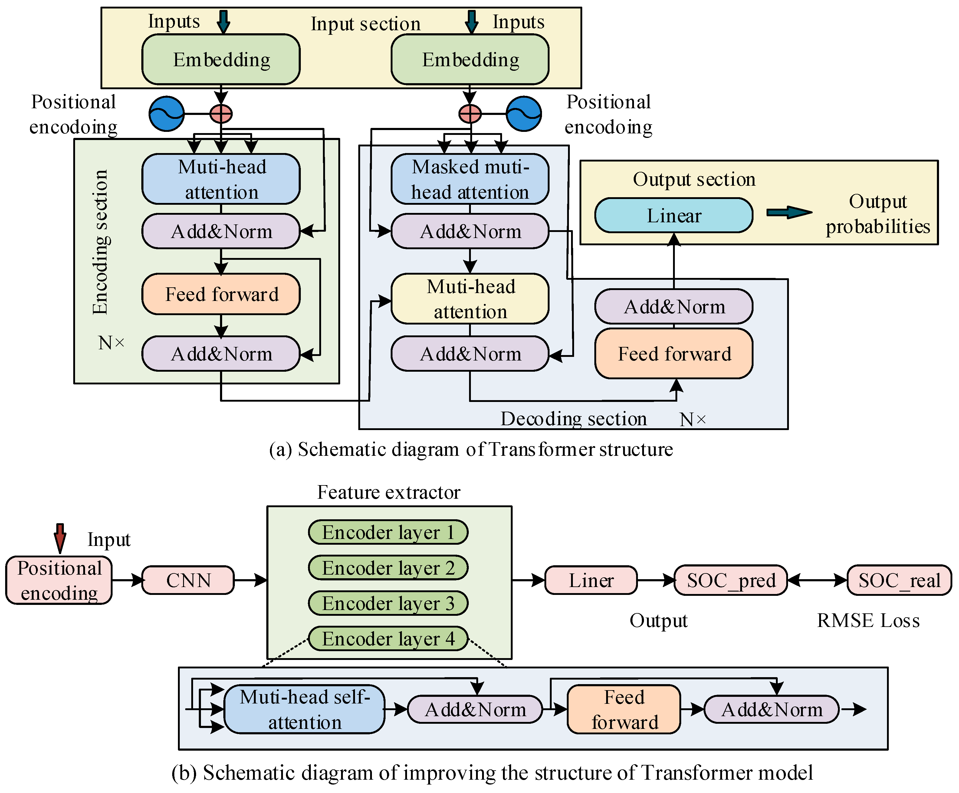
Figure 1a denotes the schematic structure of the Transformer model.
As shown in
Figure 1a, the input of the Transformer model is transmitted to the encoder–decoder through positional encoding. The encoder consists of N stacked layers, each layer containing a multi-head SAM and a feedforward neural network, and it employs residual connections and layer normalization. The decoder is also composed of N stacked layers. In addition to the above mechanism, it also adds a multi-head attention sublayer for processing the encoder output and performs masking processing [
20,
21]. To better handle long time series data, improvements have been made to the basic Transformer model structure. Improving the Transformer model includes six parts: input, position encoding, local feature extraction, encoder stacking layer, fully connected layer, and output prediction.
Figure 1b denotes the schematic structure of the improved Transformer model. In the natural language processing, the input data for Transformer models is word vectors, which transform the original word representations into linear combinations of features through input embedding methods. The CNN structure is used in
Figure 1b because the time series data of lithium batteries are essentially one-dimensional signals, and their local fluctuations contain rich dynamic features. The convolution operation of CNN can extract local correlations of temporal data through sliding windows, reducing the number of parameters by 70% compared to fully connected layers. At the same time, the weight sharing mechanism of one-dimensional convolution kernels can effectively suppress overfitting, making it more suitable for the non-stationary characteristics of battery data. When determining the parameters of the model, the kernel size is determined to be 3 and the step size is 1 through cross validation to preserve complete temporal information and avoid feature loss. The layers are stacked using two-layer convolution, with the first layer extracting basic features and the second layer fusing multi-scale features. In the setting of sliding window parameters, the window size is mainly set to 128, covering the battery thermal time constant. The step size is set to 16 to balance real-time performance and data overlap rate. When the sampling rate is 1 Hz, the 128-point sequence corresponds to 128 s, meeting the feature capture requirements under dynamic stress testing conditions.
In
Figure 1b, in the input part of the improved Transformer model, the voltage, current, and temperature in the time series are mainly used as input data for battery state estimation. For ease of use, it is necessary to preprocess and normalize the input data, convert it into a linear combination of features, and use the current estimated true value of the battery state as the input label. Specifically, it is necessary to use a sliding window method to read preprocessed data, pair it with the current battery state estimation data, and form an input and label pair. From this, the input vector calculation method for improving the Transformer model can be derived as denoted in Equation (1).
In Equation (1),
means the model input vector,
means the voltage at time step t,
denotes the current, and
denotes the temperature. Position encoding is responsible for adding positional information to each data point in the sequence, ensuring that the input data carries corresponding positional features. The Transformer model itself does not have the ability to learn sequence information, so it needs to actively provide location information to the Transformer model. The process of position encoding requires the combination of input data and corresponding sequence information to ensure that the model learns the sequence order and temporal characteristics. The specific calculation is denoted in Equation (2).
In Equation (2),
represents the preprocessed temperature, voltage, and current, with values of [0, 1];
represents the training data of the feature extraction layer; and
represents the position encoding data. The sum of the original input data and position encoding is the data for feature extraction. When selecting the position encoding method, if integer encoding is used, the value of the position encoding will be an integer from 0 to t. This method may affect the feature extraction performance due to the expansion of encoding values [
22]. Therefore, a more suitable choice is to use sine–cosine encoding, which can limit the value of position encoding within [0, 1]. In the feature extraction section, it includes local and global feature extractions. The former mainly uses a one-dimensional convolution operation, while the latter uses a SAM. One-dimensional convolution is mainly utilized to process time series data. Its basic principle is to use a convolution kernel of length
k to slide on a one-dimensional input sequence, multiply each subsequence with the convolution kernel and sum them to obtain a scalar value, and finally output a new sequence. The calculation of one-dimensional convolution is denoted in Equation (3).
In Equation (3),
represents the convolution kernel and
represents the input sequence.
represents the starting position of the sliding window. Since each convolution kernel generates a scalar, the amount of convolution kernels determines the number of channels in the output sequence. One-dimensional convolution can effectively extract frequency components of input sequences and trends of time series. By stacking multiple convolutional layers, more abstract features can be gradually learned. The dataset used in this study is the temperature, voltage, and current data of lithium batteries in energy storage power stations in a time series, all of which belong to one-dimensional signals. The process first extracts local features of the input data through one-dimensional convolution and then further extracts global features through the decoder module, effectively mining important information in time series data. The decoder consists of a stack of four feedforward networks and self-attention modules. Feedforward networks mainly enhance the computational performance of self-attention modules through linear transformations [
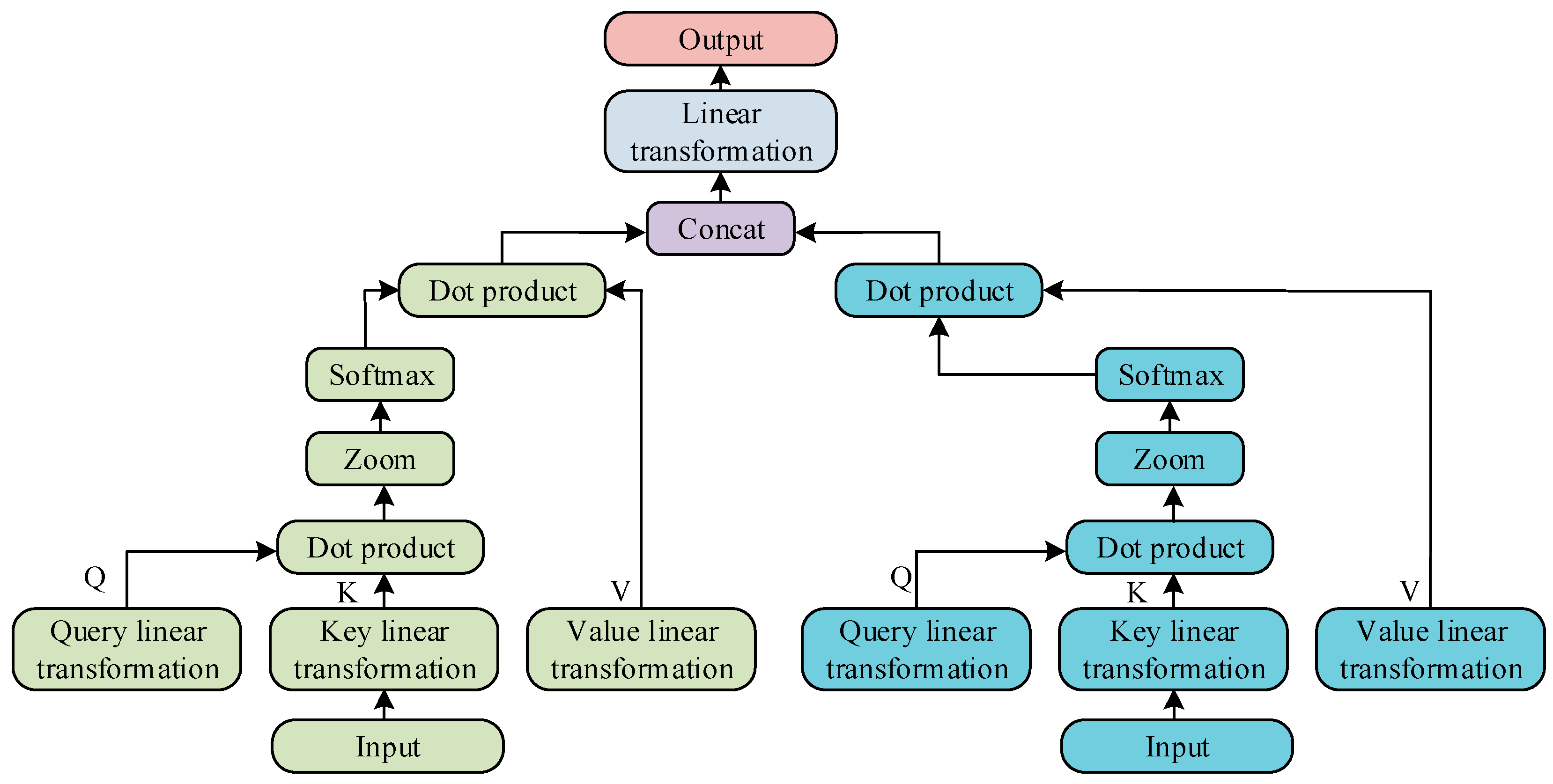
23]. Due to the extraction of local feature vectors from the input data, it is necessary to improve the original self-attention module to better meet the requirements of battery state estimation. This study mainly uses multiple attention heads to capture different correlations. The detailed explanation of the dual-head SAM is denoted in
Figure 2.
In
Figure 2, in the dual-head SAM, the input data is represented by two vectors, each vector undergoes dot product scaling through query and key linear transformations, and the output vector is generated using the softmax function. Next, compute the dot product of the output with the vector after linear transformation of the value. Finally, the output results of the two input vectors are concatenated and linearly transformed to obtain the final output vector. The dual-head SAM can effectively capture the deep relationships between input data and enhance the correlation between data [
24]. In LIBs of energy storage power plants, there is a strong correlation between data at different time points under mixed operating conditions. The dual-head SAM can fully explore the inherent connections of this long sequence data under complex operating conditions, which is conducive to improving the model’s understanding and modeling ability of complex relationships. The main advantage of the dual-head self-attention mechanism over the single-head self-attention mechanism is that it can simultaneously capture multiple correlation patterns in the input data. In battery state estimation, the model can simultaneously focus on the different effects of temperature and current on SOC, thus gaining a more comprehensive understanding of the dynamic characteristics of the battery. In addition, using the dual-head SAM can improve the modeling ability of the model for complex battery behavior without significantly increasing computational complexity. In the training process of the model, RMSE is used as the loss function, and its calculation is denoted in Equation (4) [
25].
In Equation (4),
means the actual value of the SOC,
means the predicted value of the SOC,
means the size of the input data, and
means the time point of the input data. After each training session, the RMSE optimizer is used to update weights and biases to improve the loss function’s convergence speed. Among them, the update calculation of weights is denoted in Equation (5).
In Equation (5),
represents weight and
represents a small change in weight.
represents the learning rate using to control the update step size,
represents the weighted average of the squared gradients of weights, and
is a very small constant. Among them, the calculation of
is denoted in Equation (6).
In Equation (6),
represents the gradient accumulation index, and
represents the attenuation factor used to update
. The updated expression for bias is denoted in Equation (7).
In Equation (7),
represents bias,
represents the weighted average of the squared gradients of bias, and
is calculated as denoted in Equation (8).
In Equation (8), represents the attenuation factor used to update .
2.2. State Estimation and Battery Life Prediction Methods for LIBs
In the previous section, to better process the time series data of LIBs in energy storage power plants, the traditional Transformer model structure was improved. This study mainly adopts a dual-head SAM to capture deep level correlations in input data and enhance the correlation between data. In this improved Transformer model, the input data is provided in the form of a sequence consisting of a series of time step data, where the last data point of each sequence corresponds to an estimated value of the SOC [
26,
27]. But this model makes it difficult to process future information, which reduces the accuracy of state estimation for LIBs in energy storage power plants. To solve this problem, a Transformer–TDSE model was proposed by combining the Time Delay Second Estimation algorithm to construct the time series data of the model. The core idea of TDSE is to construct a historical sequence and a sequence containing future data, to perform a secondary estimation of the true SOC values in the past at the current time, and use this estimation to correct the SOC prediction results at the current time, in order to improve real-time performance and accuracy. At time
, in addition to the previous time series, another sequence is constructed to estimate the true state of charge value at time
, denoted as
. This study first estimates the SOC value at time
through a model and then calculates the error between it and the true value
, as shown in Equation (9).
Based on this error, the error weight
is derived, and its calculation is shown in Equation (10).
In Equation (10),
reflects the magnitude of the error, and the smaller the error, the greater the weight. Similarly, calculate the SOC estimation error and its weight at time
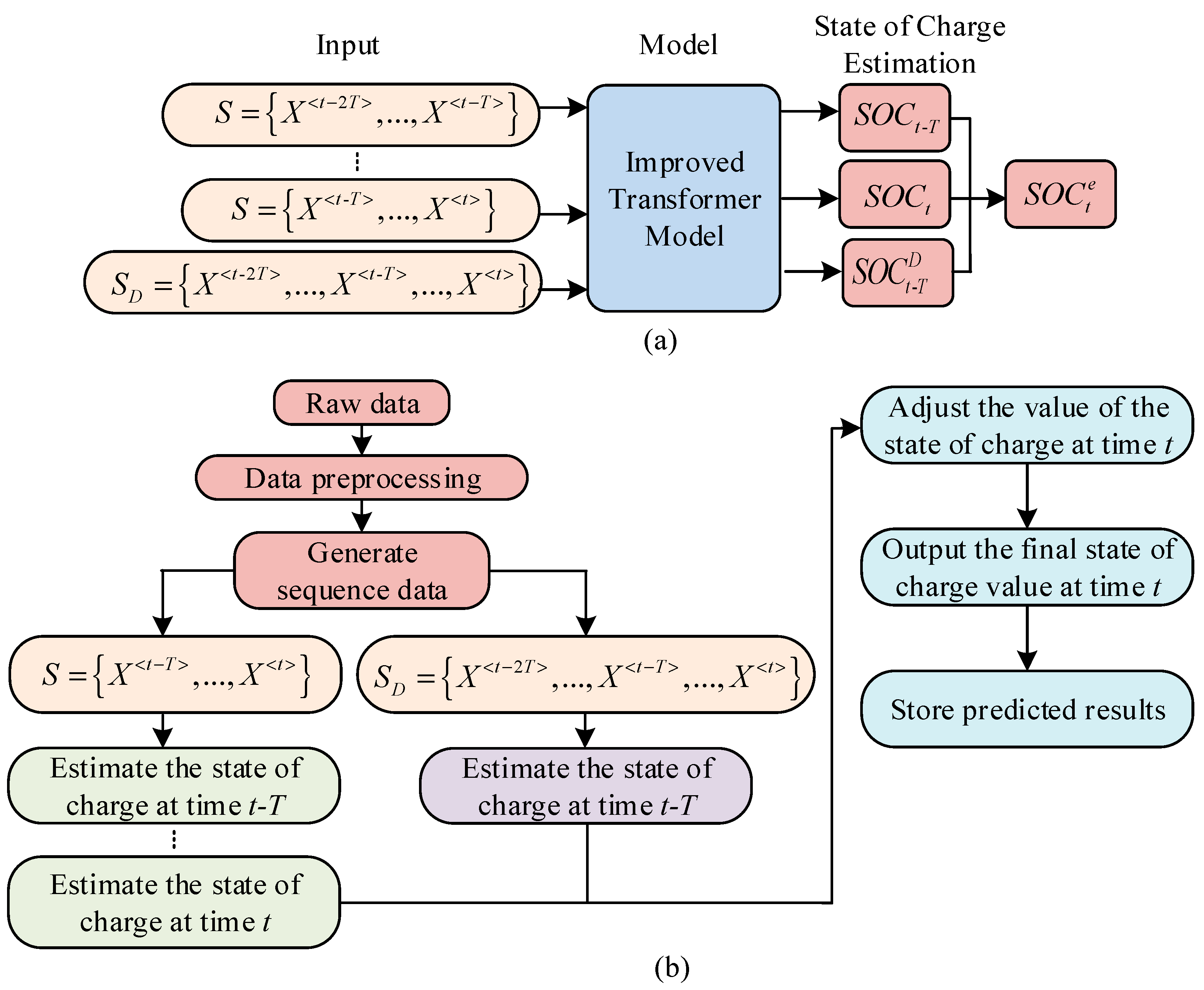
. By combining current and past estimates, the corrected SOC estimate can be obtained using the weighted average method. In this way, the Transformer–TDSE model can more accurately capture the dynamic changes during battery charging and discharging processes, adapt to different operating conditions and temperature changes, and achieve accurate SOC estimation. The schematic diagram of SOCE based on the Transformer–TDSE model is denoted in
Figure 3.
In
Figure 3a,
S represents the sequence from time
to time t, and each sequence corresponds to an estimated
SOC value.
represents an additional time series constructed at time
t, which is utilized to estimate the true SOC values at time
. Finally, by combining the estimated data from each sequence, the estimated value at time
is adjusted together to obtain
. From this, the process of estimating the SOC of LIBs in energy storage power stations based on the Transformer–TDSE model can be derived, as denoted in
Figure 3b. In
Figure 3b, the process of assessing the SOC of LIBs in energy storage power plants using the Transformer–TDSE model is to first preprocess the data, including abnormal data processing and normalization processing [
28]. Next is to construct two types of sequence data. The first type is the
S sequence, which consists of historical data and is used to assess the current SOC at time t in real time. The second type is the
SD sequence, which contains both historical data and future data, used to estimate the SOC at past times
at the current time
. Subsequently, at time
, the
S sequence and improved Transformer model are used as inputs to predict the SOC value, denoted as
. Then, at time
, the improved Transformer is used again with the S sequence and
SD sequence as inputs to estimate the SOC value at time
and the adjusted SOC value at time
. Finally, by combining the estimated values of
at time
and
, the estimated SOC value at time t is corrected to obtain the final estimated SOC value, i.e.,
. The specific operation is to first calculate the difference between the estimated values of
at time
and time
and to analyze the sources and characteristics of the error. Then, based on the results of error analysis, different weights are assigned to the two estimated values. If the error of an estimated value is small, a higher weight is assigned. Subsequently, the two estimated values are weighted and averaged according to the assigned weights to obtain the corrected
.
Normally, after multiple charge and discharge cycles, the performance of LIBs will gradually decline. Therefore, developing an efficient battery management system has become crucial [
29,
30]. Accurately predicting a battery’s SOC allows the system to understand the battery’s current condition, enabling efficient battery management. This method can prevent the shortening of battery life caused by overcharging or over-discharging, while also avoiding safety accidents caused by battery overheating. In addition, accurate estimation of battery RL also plays an important role in the development of battery management systems. Among them, the remaining battery life reflects the health level of the battery and can predict the remaining number of rechargeable and dischargeable cycles of the battery. In addition, battery capacity directly affects the accuracy of SOC estimation, as changes in battery capacity can affect the amount of energy stored and released by the battery during charging and discharging processes. As the battery is used and aged, the actual capacity of the battery will gradually decline, making SOC prediction of the battery more complex. The capacity decline of the battery will increase the prediction error of the SOC and affect the prediction of remaining life. This study mainly uses the PF algorithm for RLP of batteries, which can effectively achieve nonlinear state estimation. Due to the influence of factors such as temperature changes, charging and discharging rates, and usage frequency during the use of batteries, their degradation process is not linearly predictable. Therefore, traditional linear prediction methods often struggle to provide sufficiently accurate prediction results. The PF represents the state space of the system by generating a set of particles that are continuously updated based on observation data and system models, and the true state of the system is estimated through weighted averaging. The weight of each particle reflects its degree of matching with the current observed data. After multiple iterations, the particle set gradually approaches the true state distribution. Therefore, the PF can effectively model and estimate the nonlinear degradation process of batteries. In the PF, each particle represents a hypothesis about the model parameters. To prevent particle degradation during the multi-step update process, state transition noise is usually introduced to make the particle update process smoother and avoid excessive concentration of particles near certain parameter values. This study mainly uses a double exponential function to model capacity degradation, which is used to characterize the decline of battery capacity over time of use. In the PF, the parameters of the double exponential function are mainly estimated as unknown state variables. The PF approximates the probability distribution of these degradation model parameters by generating a large number of particles, and it gradually updates the weights of the particles based on the observed data of the battery. The double exponential function can flexibly simulate the nonlinear and dynamic characteristics of battery capacity over time, more accurately reflecting the degradation behavior of the battery during use, enabling it to adapt to the complex changes in battery performance. Among them, the double exponential function is denoted in Equation (11).
In Equation (11),
represents the amount of electrical energy that the battery can store at a specific moment,
represents the number of times the battery undergoes charging and discharging processes, and
,
,
, and
are all undetermined parameters. The specific values depend on multiple factors such as the type, material, and working environment of the battery. The observed value of battery capacity at a given time is calculated as denoted in Equation (12).
In Equation (12),
represents Gaussian white noise,
is the observed variance, and
means Gaussian noise that follows a mean of 0 and a variance of
σ. Among them, the variance
σ is selected through cross validation method with the aim of minimizing prediction error. The posterior probability distribution expression is denoted in Equation (13).
In Equation (13),
represents the capacity sequence value,
represents the given state,
represents the posterior probability distribution of the state
after obtaining the capacity sequence
, and
represents the probability of the current state
given all capacity data.
represents the marginal probability of observation value
.
refers to the likelihood function of observing
given the state
. The normalization constant calculation is denoted in Equation (14).
The true posterior probability distribution can be obtained and calculated using Equation (15) according to the central limit theorem.
In Equation (15),
represents a variable function from 0 to 1.
means the amount of particles.
means the weight of the
th particle at time
. The estimation expression for
is denoted in Equation (16).
Subsequently,
is normalized, and Equation (17) gives the specific calculation.
The capacity degradation of batteries is not only related to the number of charge and discharge cycles but also affected by factors such as temperature, current intensity, and charge and discharge rate. Therefore, when using a double exponential model for capacity decline prediction, multiple factors need to be comprehensively considered. In addition, due to varying battery capacities, each battery has a separate failure threshold set, which ranges from 70% to 80% of its rated capacity.
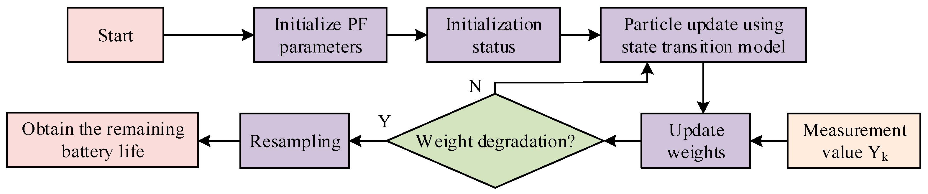
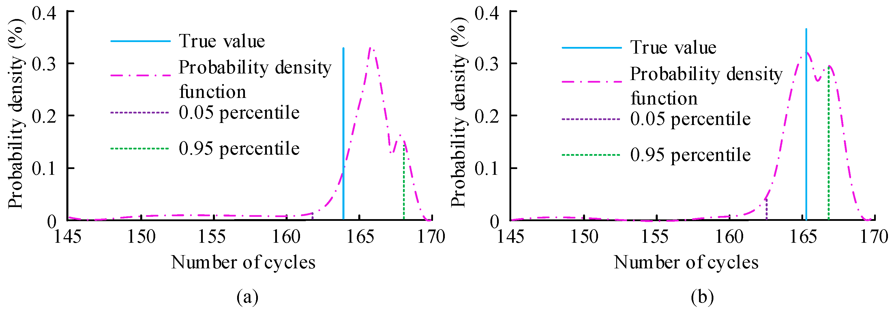
Figure 4 shows the PF algorithm flowchart.
In
Figure 4, the procedure of the PF algorithm starts by setting the initial parameters of the PF algorithm, including the number of particles, initial state, and observation model parameters. The initial state is set, including initial state estimation and weights. Then, a state transition model is utilized to update the state of each particle. Subsequently, new measurement values are obtained at each time step, and the weights of each particle are updated based on the new measurement values and observation model. Next, it is checked whether the particle weights are decreasing, i.e., whether the number of valid particles is below the set failure threshold. If so, resampling is performed. If not, it will calculate and update the particles until the particle weights degrade. The difference between the actual capacity degradation to the failure threshold cycle times and the set cycle times is used to obtain the remaining battery life.
2.3. Data Source Description
The experimental data was obtained from 5 ternary lithium batteries (rated capacity 2.0 Ah) and 5 lithium iron phosphate batteries (rated capacity 2.5 Ah), each battery completed 200–500 charge and discharge cycles, and a total of 16,800 time series samples including voltage, current, temperature, and SOC true values were obtained. The data collection covered operating conditions from −10 °C to 50 °C, including multiple operating conditions. The Arbin BT2000 battery testing system was used for data acquisition, with a sampling rate of 1 Hz. Temperature control was achieved through a constant temperature box with a stability of ±0.5 °C. Real-time recording of battery terminal voltage, charging and discharging current, and surface temperature during the testing process was carried out, as well as the simultaneous acquisition of SOC true values through the Coulomb counting method combined with the open-circuit voltage method. The collected data needed to undergo three-step preprocessing. Firstly, the 3σ principle was used to eliminate abnormal points where the voltage deviation exceeds ±2% of the rated voltage and the current deviation exceeds ±5% of the rated current. Then, the eigenvalue domain was mapped to [0, 1] through minimum–maximum scaling. Finally, the sliding window method was used to construct an input label pair, where the input was the voltage, current, and temperature sequence within the window, and the label was the SOC value at the end of the window. The model was trained using the Adam optimizer with a learning rate of 1 × 10⁻⁴, β1 = 0.9, and β2 = 0.999. The batch size was 32 and the training epochs were 100. The network structure consisted of 4 hidden layers, with 8 attention heads set in each layer. To avoid overfitting, an early stopping strategy was introduced with a patience value of 10, which means that if the validation set loss did not decrease for 10 consecutive rounds, training was terminated.
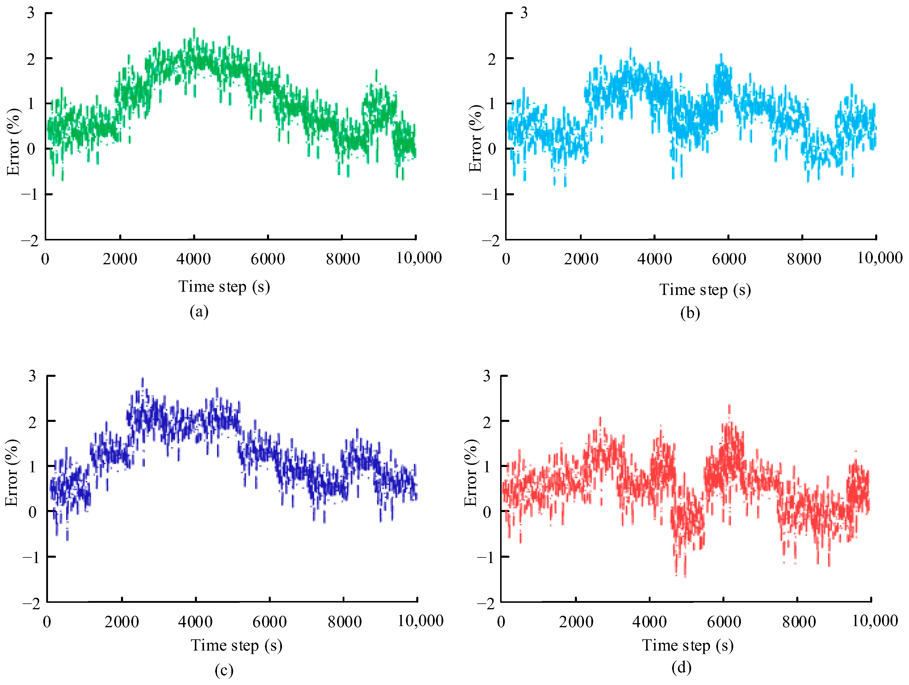
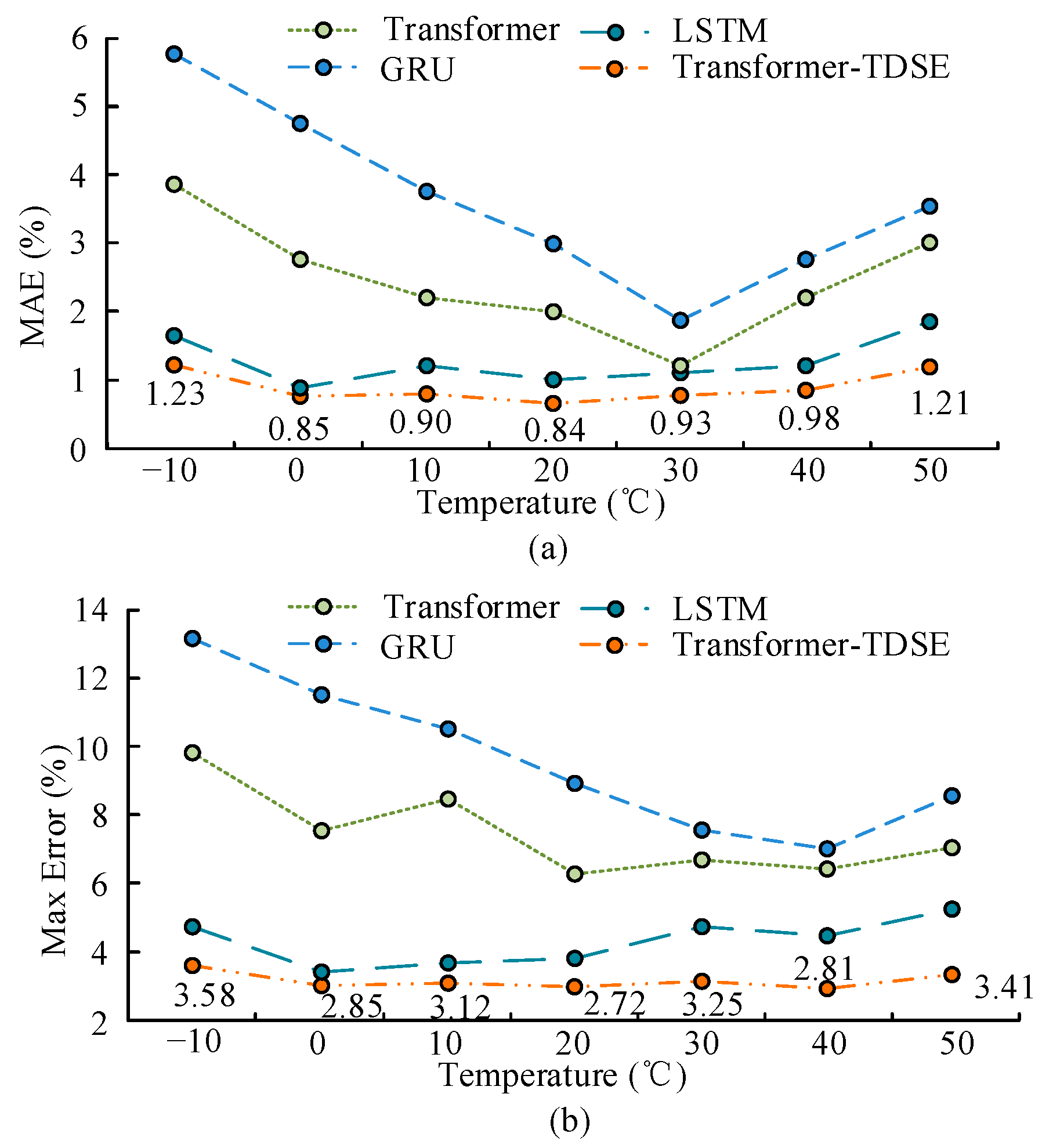
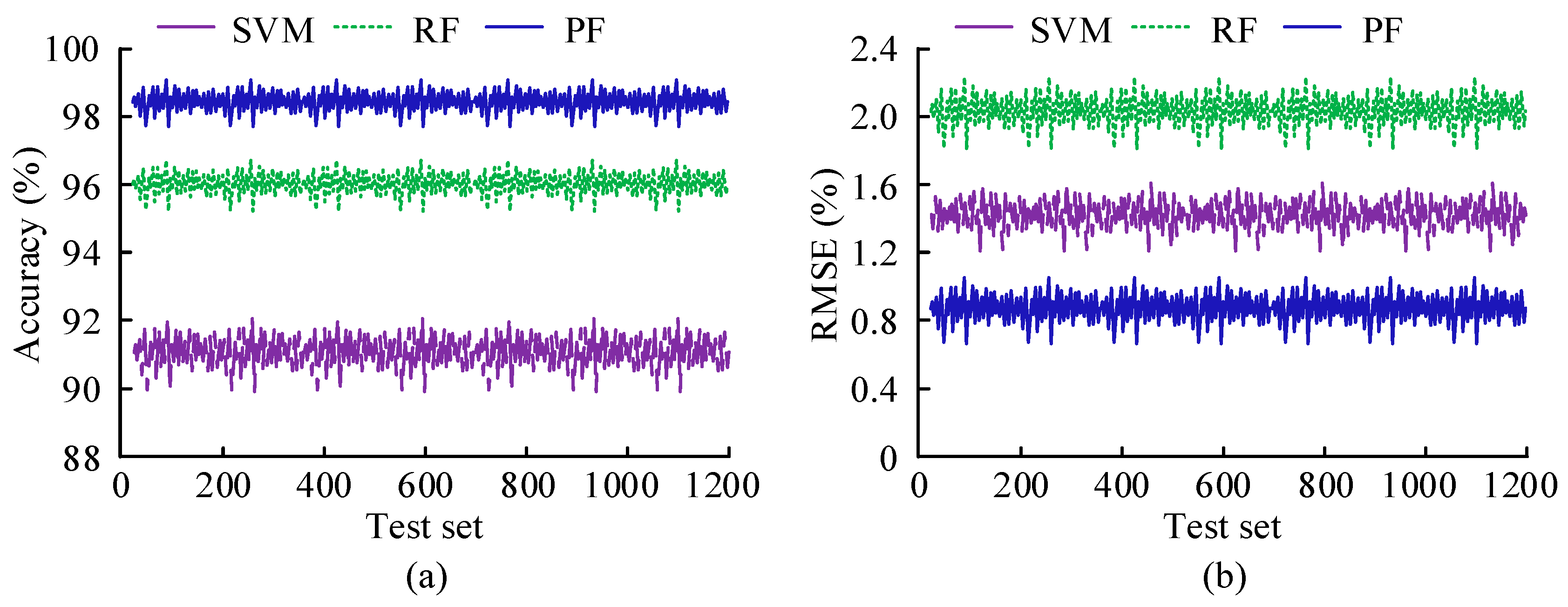
In the baseline comparison, the MAE of the Kalman filter at 10 °C was 0.95%, the PF algorithm was 0.88%, and the Transformer–TDSE model reduced MAE to 0.82%. Under extreme low-temperature conditions of −10 °C, Transformer–TDSE reduces MAE from 1.82% to 1.25% compared to the Kalman filter, verifying its adaptability to complex working conditions.


