GITT Limitations and EIS Insights into Kinetics of NMC622

Abstract

Conventional applications of the Galvanostatic Intermittent Titration Technique (GITT) and EIS for estimating chemical diffusivity in battery electrodes face issues such as insufficient relaxation time to reach equilibrium, excessively long pulse durations that violate the short-time diffusion assumption, and the assumption of sequential electrode reaction and diffusion processes. In this work, a quasi-equilibrium criterion of 0.1 mV h⁻¹ was applied to NMC622 electrodes, yielding 8–9 h relaxations below 3.8 V, but above 3.8 V, voltage decayed linearly and indefinitely, even upon discharging titration, showing unusual nonmonotonic relaxation behavior. The initial 36-s transients of a 10-min galvanostatic pulse and diffusion impedance in series with the electrode reaction yielded consistent diffusivity values. However, solid-state diffusion in spherical active particles within porous electrodes, where ambipolar diffusion occurs in the pore electrolyte with $t_{+}=0.3$, requires a physics-based three-rail transmission line model (TLM). The corrected diffusivity may be three to four times higher. An analytic two-rail TLM approximating the three-rail numerical model was applied to temperature- and frequency-dependent EIS data. This approach mitigates parameter ambiguity and unphysical correlations in EIS. Physics-based EIS enables the identification of multistep energetics and the diagnosis of performance and degradation mechanisms.

1. Introduction

Introduced by Weppner and Huggins [1,2,3], the Galvanostatic Intermittent Titration Technique (GITT) has gained widespread acceptance to assess chemical diffusivity in battery electrode materials as a function of the state of charge (SOC). Currently, there are several issues in conventional GITT practices.

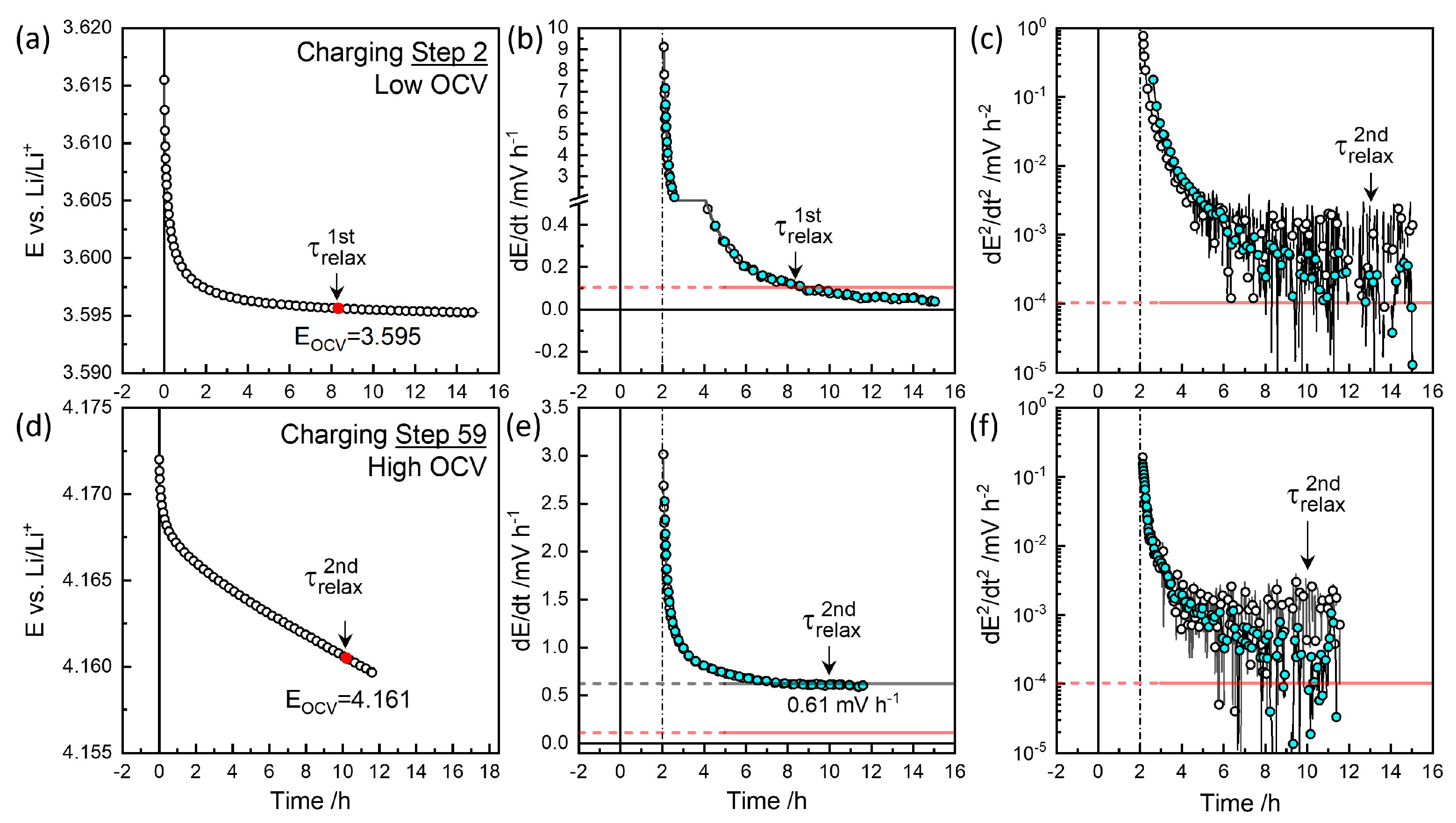
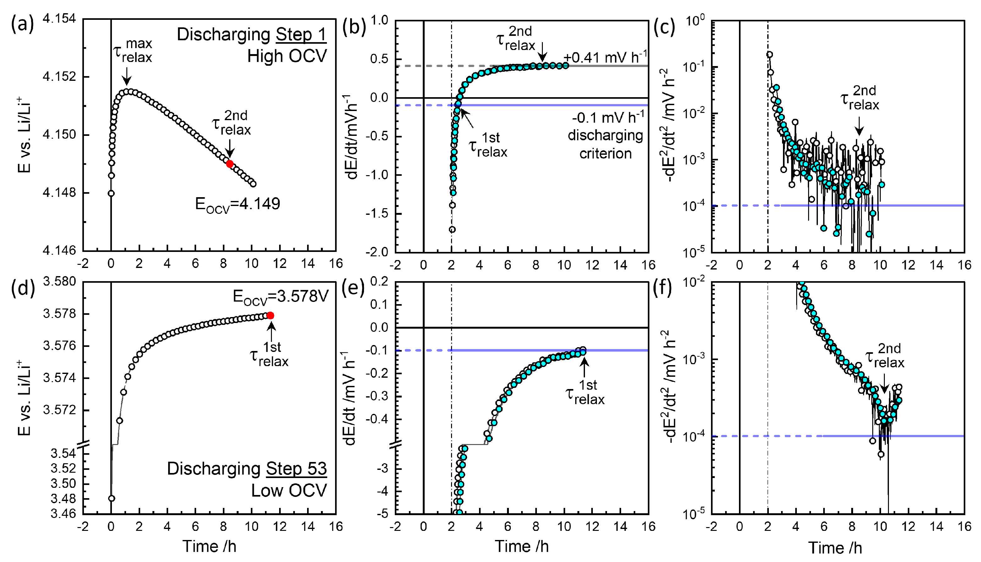
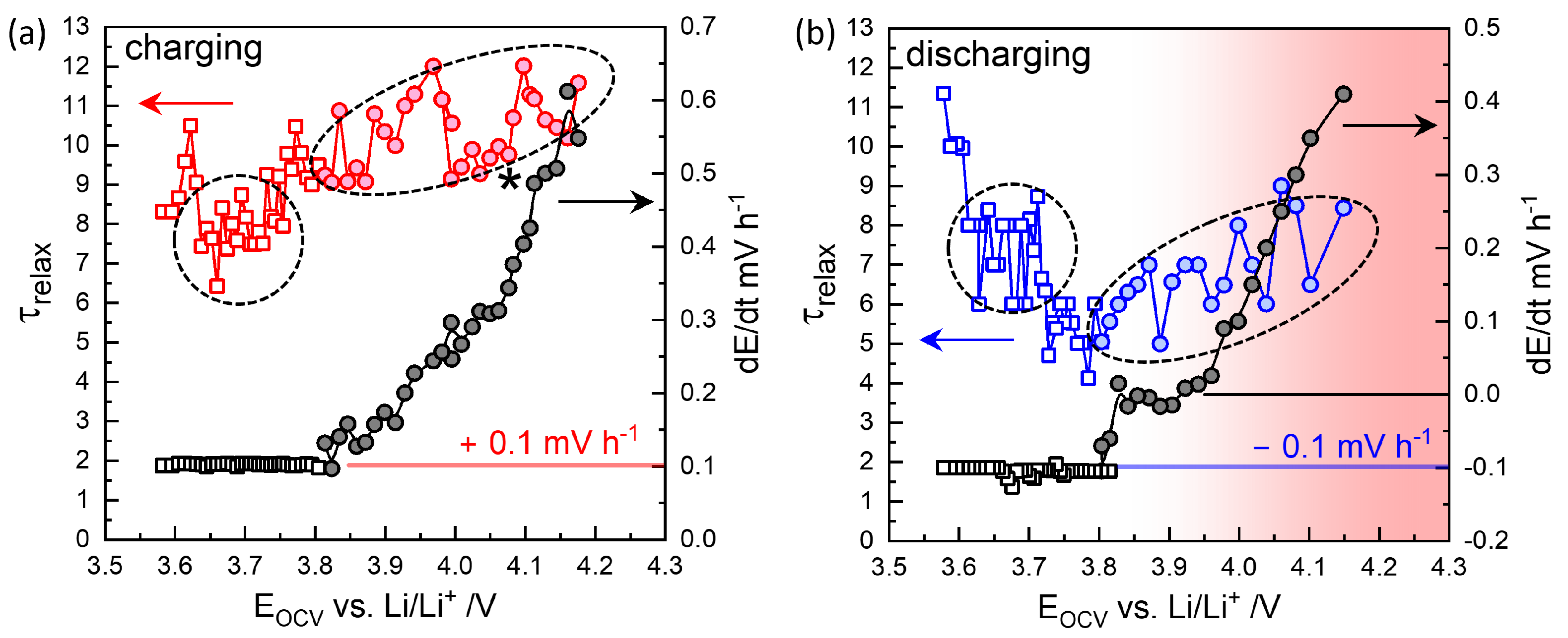
• Relaxation periods ${\tau }_{\mathrm{relax}}$ are typically set to a constant (e.g., 1 h [4,5,6,7,8]) in automated procedures provided by commercial potentio/galvanostats. However, these fixed relaxation times do not guarantee the attainment of equilibrium open-circuit voltages (OCVs), which is one of the main purposes of the GITT.
• The titration pulse ${\tau }_{\mathrm{p}}$ must be short enough for the widely used relation from the $\sqrt{t}$ dependence [1,3]. In many studies, the entire SOC range of battery electrodes, not the narrow regions of solid solution [1,2,3], is titrated. With a 0.1 C current, the pulse duration of 1 h requires 10 steps, 10 min 60 steps, and 1 min 600 steps. The pulse duration can be too long for the equation based on the short-time solution.
• The original GITT kinetic analysis was developed for thin-film electrodes for one-dimensional solid-state diffusion. However, the analysis has been widely used for battery electrodes, where the active material particles are dispersed and the pores between them are filled with the electrolyte. A three-dimensional spherical diffusion occurs for the individual particles, and the liquid-phase diffusion in the electrolyte is also present.
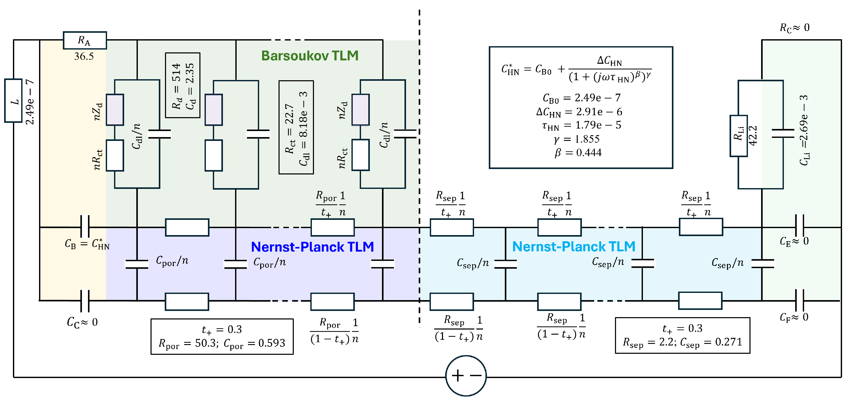
• The Randles circuit, originally used for the diffusion of redox species in the electrolyte [9], was used to determine the chemical diffusivity in thin-film electrodes by electrochemical impedance spectroscopy (EIS) [3,10]. While the Warburg response in the Randles circuit is an $RC$ transmission line model (TLM) for one-dimensional diffusion in films, distributed responses in porous electrodes need to be represented by a TLM [11] that needs to incorporate solid-state diffusion in dispersed spherical particles.

In the present work, the GITT and EIS are combined to investigate the thermodynamic and kinetic properties of LiNi_0.6Mn_0.2Co_0.2O₂ (NMC622). EIS measured at equilibrium can be compared with the GITT analysis of the voltage transients upon the subsequent current pulse. For NMC622 (and also NMC811) electrodes, equilibrium OCVs are not reached at high OCVs; the voltage decay linearly for several dozens of hours. The relaxation behavior is studied systematically, revealing characteristic kinetics that depend on the OCV.

The pitfalls of the conventional GITT and EIS analysis for porous battery electrodes are carefully demonstrated. Although the transients for the GITT analysis and the frequency response of the EIS are equivalent, the EIS is shown to be superior in obtaining and modeling the multiscale time response. The aspects of porous electrodes with solid-state diffusion in dispersed active material particles and diffusion in the electrolyte with Li⁺ transference number, $t_{+}\approx 0.3$ can be described by a three-rail TLM requiring numerical calculations [12,13,14]. An analytic two-rail TLM is devised, which allows the least-squares fitting analysis [15,16]. Furthermore, inevitable and troublesome parameter correlations in the least-squares fitting optimization are shown to be overcome by a temperature-dependent multi-data fitting analysis [16,17,18].

2. Cell Preparation, Electrochemical Characterization, and Data Analysis

Coin cells were prepared following the standard laboratory process, as illustrated in Figure S1. Commercial NMC622 powder (Umicore, Cheonan, Republic of Korea) with an average particle size of 5.07 ± 0.97 μm, as determined by SEM (Figure S2), was thoroughly mixed with conductive carbon black (EQ-lib-Super65, MTI Corp., Richmond, CA, USA) and polyvinylidene fluoride (PVDF; Mv = 600,000, MTI) binder in N-Methyl-2-pyrrolidone (NMP; 99%, Sigma-Aldrich, St.Louis, MO, USA) in a weight ratio of 8:1:1, respectively. The mixture was uniformly coated onto aluminum foil using a doctor blade set to 180 μm. Subsequently, the coated foil was dried in vacuum at 80 °C for 12 h.

The dried electrode film was calendared twice, to 80% and then to 65% of its initial thickness (117 μm), before being cut into 14 mm diameter discs. Each cell contained approximately 3 mg of active material, and the calculation of the C rate was based on an assumed capacity of 180 mAh g⁻¹ [19,20].

Each cell was configured in a CR2032 coin cell, consisting of the working electrode, a separator (3501, Celgard^®, 25 μm, Charlotte, NC, USA), and a 16 mm diameter lithium fill electrode. A total of 50 μL of electrolyte containing 1 M lithium hexafluorophosphate (LiPF₆; 99.99%, Sigma-Aldrich) in ethylene carbonate (EC; 98%, Sigma-Aldrich) and dimethyl carbonate (DMC; 99%, Sigma-Aldrich) in a 1:1 volume ratio was introduced into the separator. All cell fabrication procedures were performed in an argon-filled glovebox. The assembled cells were aged at 25 °C for 18 h before electrochemical testing.

The electrochemical test setup is shown in Figure S3. The coin cells were loaded into a Peltier chamber (Memmert IPP30plus, Schwabach, Germany) set at 30 °C using a 10-coin cell holder (Neoscience, Seoul Republic of Korea). The temperature variation in the cells during battery testing was continuously measured using K-type thermocouples attached directly to the top of the cells. Electrochemical measurements were conducted using a Biologic VSP300 potentiostat (BioLogic, Seyssinet-Pariset, France) with the dedicated EC-Lab^® software ver. 11.60.

The electrochemical test procedures are shown in Figure 1. After formation cycles and once (quasi-)equilibrium was reached, EIS measurements were performed from 1 MHz to 0.01 Hz for 34 min (2-cycle average). Each galvanostatic titration lasted for 10 min (${\tau }_{\mathrm{p}}$) and was followed by indefinite relaxation periods until the next equilibrium SOC was attained, at which point EIS measurements and subsequent titrations were conducted.

Figure 1. Electrochemicalmeasurement procedures. After formation cycles and once (quasi-)equilibrium is reached, EIS is measured from 1 MHz to 0.01 Hz, followed by a 10-min galvanostatic titration (${\tau }_{\mathrm{p}}$) and an indefinite relaxation period until the next SOC equilibrium. Relaxation periods (${\tau }_{\mathrm{relax}}$) are determined based on quasi-equilibrium criteria: 0.1 C at equilibrium and either $dE/dt=0.1$ mV h⁻¹ or $d^{2}E/d{t}^2={10}^{-4}$ mV h⁻².

For the cell after months-long GITT cycles, temperature-dependent EIS was performed using a multisine method, measuring down to 1 mHz over approximately 17 min at selected temperatures ranging from 5 °C to 60 °C in 5 °C increments at an OCV of 3.696 V.

For clarity, the large datasets presented in the figures were processed using the appropriate “Smart Skip” methods in OriginLab^® 2023 (OriginLab Corporation, Northampton, MA, USA).

The impedance analysis and simulations were performed using in-house Python scripts. The first script was for the numerical simulation of the 3-rail transmission line model [12,13], which is now publicly available in ref. [14]. The second script was for the least-squares fitting of any analytical models [16,17,18], which was compared with ZView^® Ver. 4.0 (Scribner Associates Inc., Southern Pines, NC, USA) when the corresponding models were provided in the commercial program. An approximate analytical model of the recently developed 3-rail TLM [15,16] was used for the least-squares fitting analysis. The third script was for the temperature and frequency dependence using multiple EIS data at different temperatures [16,17,18].

3. Galvanostatic Intermittent Titration Technique

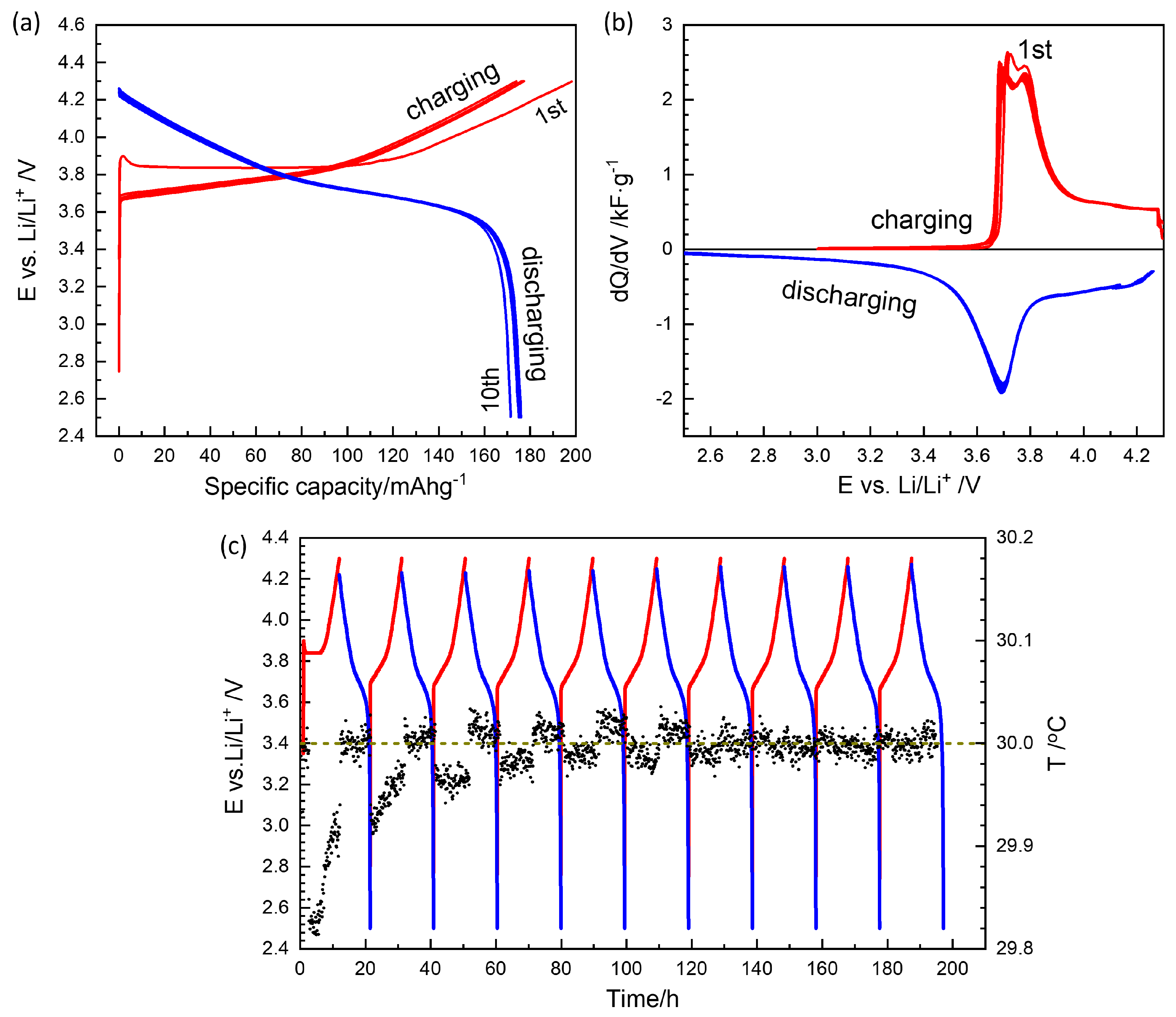
3.1. Formation Cycles

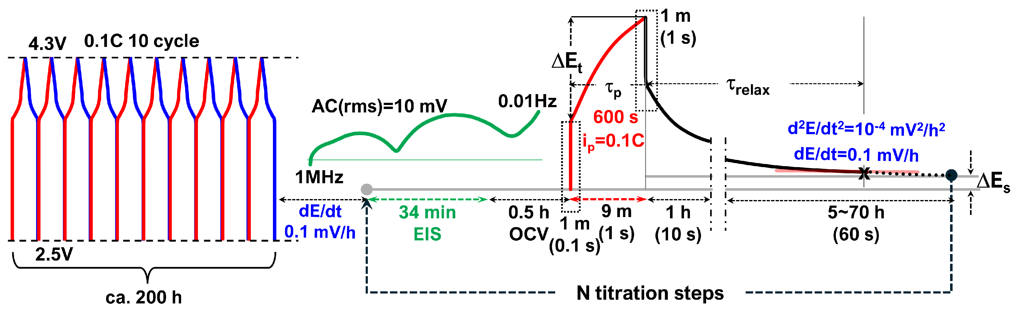
Ten consecutive charge–discharge cycles stabilized fresh cells at a 0.1 C rate (54.4 μA) between 2.5 V and 4.3 V, as shown in Figure 2. The first charge cycle typically exhibited a high capacity of 200 mAh g⁻¹, which can be attributed to SEI formation. The capacity then stabilized close to the nominal value of 180 mAh g⁻¹ (Figure 2a).

Figure 2. (a) The first 10 charge/discharge cycles of a Li-NMC622 coin cell. (b) Differential capacity curves. (c) Charge/discharge potential and temperature in circles as a function of time. Red and blue lines are for charging and discharging, respectively.

The differential capacity curves in Figure 2b clearly show the asymmetry between charge and discharge. The presence of two split peaks in the charge profile and a single peak in the discharge profile is characteristic of high-nickel compositions above NMC622 [4,21]. While charging started above 3.7 V, the discharge curve gradually shifted below the peak at approximately 3.7 V.

The setup used in this work (Figure S3) enabled in situ temperature monitoring of each battery cell (Figure 2c). In coin cells, endothermic/exothermic heat effects during charge/discharge and Joule heating are minimal and indistinguishable from noise. However, endothermic heat effects associated with SEI formation were observed during the first charge cycles, supporting the application of three to five SEI formation cycles. The observed endothermicity of the SEI formation reaction may be attributed to the decomposition of solvent molecules.

3.2. GITT Overview

Figure 3 (left) presents the raw voltage data for 900 h of the 60 titration steps during charging and 600 h of the 53 steps during discharging, totaling approximately 1500 h (62 days). Galvanostatic pulses ($i_{\mathrm{p}}$ = 54.4 μA), corresponding to 0.1 C for the active material mass of 3.02 mg, were applied for 10 min, which is 1/60 of the nominal capacity of 180 mAh g⁻¹. The measured discharge capacity was reduced from 180 mAh g⁻¹ to 159 mAh g⁻¹.

Figure 3. Potential vs. Li⁺/Li during charging and discharging titration as a function of time (left) and capacity (right). Circle symbols indicate (quasi-)equilibrium OCV points. Charging titration steps 2 and 59 correspond to Figure 4, while discharging steps 1 and 53 correspond to Figure 5. Step 46 is used as the representative data for the main analysis and discussion. See the text for the magnified inset with an asterisk.

The voltage cutoff was set between 2.5 V and 4.2 V; however, a stable OCV for the GITT was only achieved above 3.6 V, as indicated by the circle symbols. The small red and blue points or lines represent the voltage during titration and relaxation, respectively. The unequal spacing of OCV points, due to irregular relaxation periods, is a distinguishing feature of this study. In most GITT studies, both the relaxation and titration periods are fixed, as detailed below. Figure 3 (right) shows the voltage as a function of capacity. The red points in Figure 3 (left) more clearly show the time dependence of the voltage during galvanostatic titration.

The voltage recording intervals were dynamically adjusted:

• First minute: 0.1 s intervals (600 data points) to capture the fast initial voltage change.
• Next 9 min: 1 s intervals (540 points), resulting in a total of 1140 data points per titration step.

Immediately after the titration current was turned off, the voltage relaxation was recorded at the following intervals:

• Every second for 1 min (60 points) to capture the fast initial response.
• Every 10 s for 1 h (360 points).
• Every minute thereafter for long-term relaxation monitoring.

Relaxation to equilibrium was initially monitored indefinitely until the criterion $dE/dt=0.1$ mV h⁻¹ was met. That period was defined as ${\tau }_{\mathrm{relax}}^{1\mathrm{st}}$. At high OCV, the primary criterion was not met even after several tens of hours. In such cases, relaxation monitoring was stopped based on a secondary criterion, $d^{2}E/d{t}^2={10}^{-4}$ mV² h⁻², which defined the characteristic relaxation time ${\tau }_{\mathrm{relax}}^{2\mathrm{nd}}$. After satisfying either the first or second criterion, EIS measurements were conducted from 1 MHz to 10 mHz using an AC rms voltage of 10 mV with respect to OCV, before applying the next titration pulse.

3.3. GITT for Equilibrium OCVs

In most GITT studies, relaxation periods are fixed by automated sequences: 40 min [22,23], 120–135 min [24], 1 h [4,5,6,7,8], 1.5 h [25], 2 h [26,27], 3 h [23,28], 4 h [29,30,31,32,33,34], 5 h [35,36,37,38], 6 h [39], 10 h [40,41], 12 h [39], and even a day or longer [39,42]. Kim et al. [43] reviewed cases from 40 min to 10 h.

Figure 4 and Figure 5 show the relaxation behavior of the selected steps. The raw data were recorded every minute, and the “Smart Skip” function in OriginLab^® was used for clarity. Slow relaxation becomes perceptible only over prolonged periods, necessitating a criterion such as $dE/dt=0.1$ mV h⁻¹ [44]. The cutoff control $dE/dt$, available in EC-Lab^® for automated procedures, was ineffective for slow relaxation at $dE/dt=0.1$ mV h⁻¹ due to noise. Instead, the relaxation time ${\tau }_{\mathrm{relax}}^{1\mathrm{st}}$ for this cutoff was evaluated using:

$${\displaystyle \frac{dE}{dt}}={\displaystyle \frac{E(t-2h)-E\left(t\right)}{2}}$$

(1)

where the two-hour difference captures a significant trend over fluctuations. Estimation started after 2 h.

Figure 4. Relaxation behavior at charging steps 2 and 59 (a,d), first derivative of voltage $dE/dt$ (b,e), and second derivative $d^{2}E/d{t}^2$ (c,f) for ${\tau }_{\mathrm{relax}}$ and $E_{\mathrm{OCV}}$ in Figure 6a.

Figure 5. Relaxation behavior at discharging steps 1 and 53 (a,d), first derivative of voltage $dE/dt$ (b,e), and second derivative $d^{2}E/d{t}^2$ (c,f) for ${\tau }_{\mathrm{relax}}$ and $E_{\mathrm{OCV}}$ in Figure 6b.

Figure 4a,b illustrate charge step 2, which reached the cutoff criterion $dE/dt=0.1$ mV h⁻¹ at approximately 8.3 h, defining ${\tau }_{\mathrm{relax}}^{1\mathrm{st}}$. The colored symbols represent smoothed data for the sake of clarity. The voltage decrease was monitored for 15 h. Figure 4c shows the decay rate $d^{2}E/d{t}^2$ slowed down to ${10}^{-4}$ mV h⁻² at around 13 h, defining ${\tau }_{\mathrm{relax}}^{2\mathrm{nd}}$. ${\tau }_{\mathrm{relax}}^{1\mathrm{st}}$ was taken as the characteristic relaxation period with 3.595 V as equilibrium OCV, $E_{\mathrm{OCV}}$. Figure 5d,e depict discharge step 53, where the relaxation criterion $dE/dt=-0.1$ mV h⁻¹ was reached at 11.3 h, defining ${\tau }_{\mathrm{relax}}^{1\mathrm{st}}$ near the end of monitoring for $E_{\mathrm{OCV}}=3.578$ V. As shown in Figure 4f, the decay rate $d^{2}E/d{t}^2$ decreased and then increased again around 10 h, potentially defining ${\tau }_{\mathrm{relax}}^{2\mathrm{nd}}$.

For OCVs below approximately 3.8 V, the $dE/dt=0.1$ mV h⁻¹ criterion was applied, and ${\tau }_{\mathrm{relax}}^{1\mathrm{st}}$ is represented as open square symbols as a function of $E_{\mathrm{OCV}}$ in Figure 6. Compared to the $E_{\mathrm{OCV}}$ values in Figure 3, which correspond to the end of relaxation before the next titration step, $E_{\mathrm{OCV}}$ at ${\tau }_{\mathrm{relax}}^{1\mathrm{st}}$ was slightly higher for charging steps and slightly lower for discharging steps. As indicated by the dashed circle, around $E_{\mathrm{OCV}}\approx 3.68\pm 0.5$ V, ${\tau }_{\mathrm{relax}}^{1\mathrm{st}}$ was approximately 7–8 h.

Figure 6. Relaxation times ${\tau }_{\mathrm{relax}}^{1\mathrm{st}}$ at $dE/dt=0.1$ mV h⁻¹ (squares) below $E_{\mathrm{OCV}}$ 3.8 V and ${\tau }_{\mathrm{relax}}^{2\mathrm{nd}}$ at $d^{2}E/d{t}^2={10}^{-4}$ mV h⁻² with $dE/dt$ values increasing up to 0.56 mV h⁻¹ above approximately 3.8 V (circles) during charging (a) and discharging (b). For normal discharging in the opposite direction, $dE/dt=-0.1$ mV h⁻¹. Long-time relaxation occurs in the opposite direction (positive $dE/dt$) as in charging steps, which is indicated by the shade in red.

At high OCVs above 3.8 V, as shown in Figure 4d,e, the decay did not saturate to meet the $dE/dt=0.1$ mV h⁻¹ criterion but instead persisted nearly linearly for 12 h. Thus, a ${\tau }_{\mathrm{relax}}^{2\mathrm{nd}}$ of 10 h, for the secondary criterion $d^{2}E/d{t}^2={10}^{-4}$ mV h⁻² was chosen as the characteristic relaxation time at $E_{\mathrm{OCV}}=4.16$ V, with a decay rate of 0.61 mV h⁻¹. The charging step indicated by the star in Figure 3 was monitored for 38 h, resulting in a deviation in $E_{\mathrm{OCV}}$ from the trend. ${\tau }_{\mathrm{relax}}^{2\mathrm{nd}}$ was estimated at 9.8 h for $E_{\mathrm{OCV}}=4.077$ V (Figure 6a), while the final relaxation value was 4.067 V. $E_{\mathrm{OCV}}$ values at ${\tau }_{\mathrm{relax}}^{2\mathrm{nd}}$ are indicated in red-edged symbols in Figure 3 for comparison (see magnified insets). The difference between $E_{\mathrm{OCV}}$ values at ${\tau }_{\mathrm{relax}}^{2\mathrm{nd}}$ became more significant with extended relaxation times. Figure 6a shows that $dE/dt$ increased with OCV from 0.1 mV h⁻¹ at 3.8 V to 0.6 mV h⁻¹ at 4.1 V, where the corresponding ${\tau }_{\mathrm{relax}}^{2\mathrm{nd}}$ ranged from 9 to 12 h.

The high OCV relaxation in the discharging steps exhibited non-monotonic behavior, as shown in Figure 5a. The initial fast relaxation over 1 h (${\tau }_{\mathrm{relax}}^{\max }$) was followed by a long-term relaxation in the opposite direction, that is, as in the charging steps in Figure 4d. The obtained ${\tau }_{\mathrm{relax}}^{2\mathrm{nd}}$ values ranged between 5 and 8 h, with decay rates from $-0.1$ to +0.4 mV h⁻¹ in the opposite direction (Figure 6b). Relaxation periods and decay rates during discharging appeared to have been shifted downward from those during charging (Figure 6a).

The 60 charging steps corresponded to 180 mAh g⁻¹, the nominal capacity of NMC622 assumed in this work. The 53 discharge steps corresponded to 159 mAh g⁻¹. As the voltage decayed indefinitely at high OCV, the nominal titration was likely to overestimate the capacity. Subsequent GITT cycles of the same cell spanned 1870 h (60 charging steps) and 700 h (57 discharging steps), totaling 2570 h (107 days) (Figure S4). Similar dependencies of ${\tau }_{\mathrm{relax}}$ and $dE/dt$ on OCV were observed. Additional data for different NMC622 and NMC811 cells are shown in Figures S5–S13.

The low OCV and high OCV transition corresponds to the oxidation of Ni (Ni²⁺ → Ni³⁺ accompanied by an H1-H2 transition [8,45]. The indefinite voltage decay at high OCV, not previously noted to the authors’ knowledge, requires attention for these high-capacity, high-voltage electrode materials.

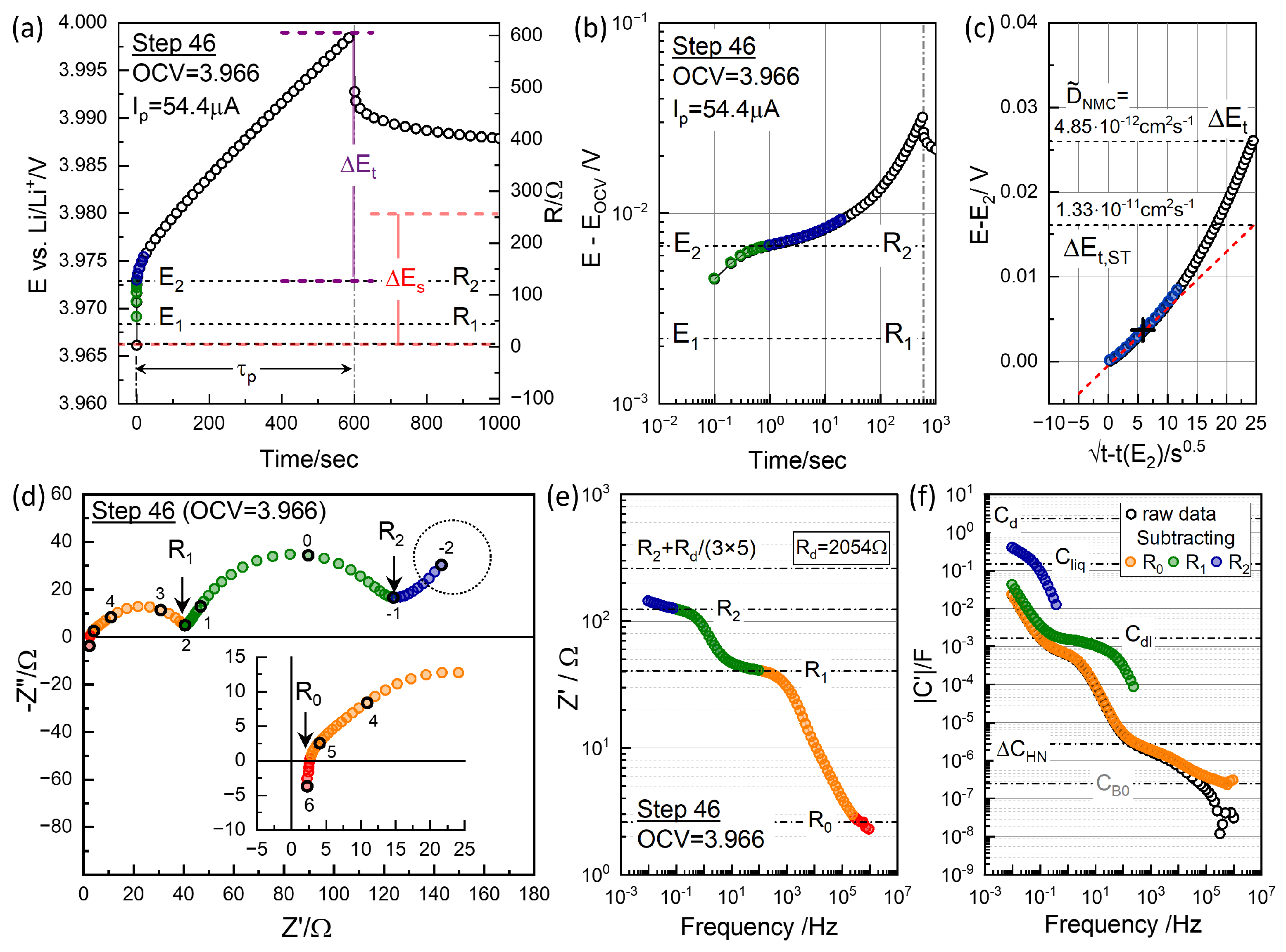
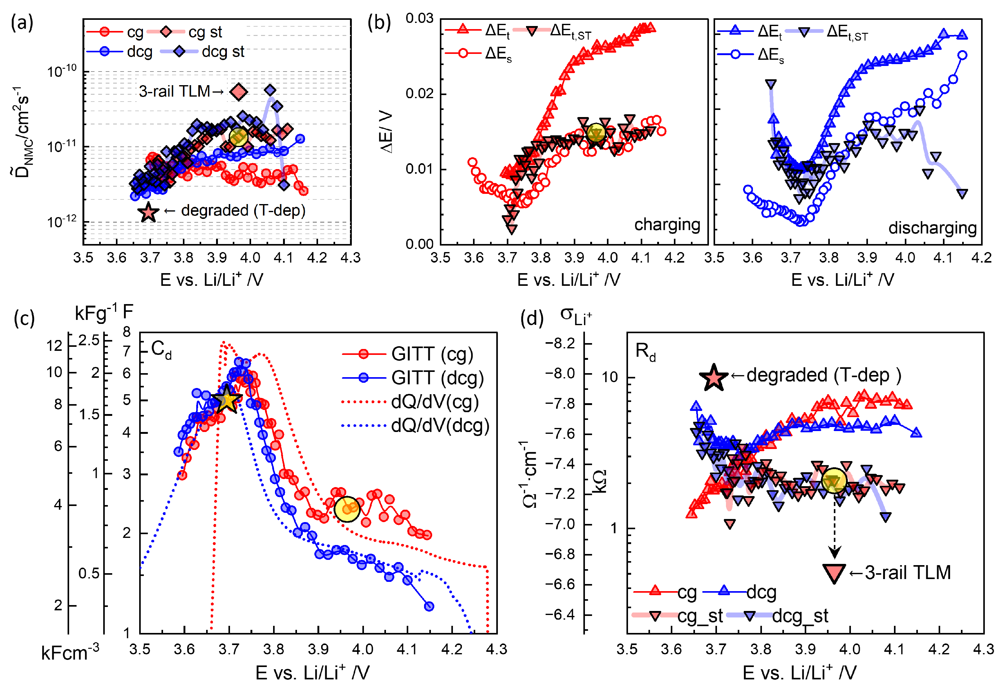
3.4. GITT for Chemical Diffusivity

Following Refs. [1,3], chemical diffusivity was estimated from the transient voltage, where the short-time solution of the diffusion equation can be applied [46,47]. The chemical diffusivity, ${\tilde{D}}_{\mathrm{NMC}}$, is given by:

$${\tilde{D}}_{\mathrm{NMC}}={\displaystyle \frac{4}{\pi {\tau }_{\mathrm{p}}}}{\left({\displaystyle \frac{m{V}_{\mathrm{M}}}{m_{\mathrm{M}}S}}\right)}^2{\left({\displaystyle \frac{\Delta E_{\mathrm{s}}}{\Delta E_{\mathrm{t}}}}\right)}^2={\displaystyle \frac{4}{\pi {\tau }_{\mathrm{p}}}}{\left({\displaystyle \frac{m}{d_{\mathrm{NMC}}S}}\right)}^2{\left({\displaystyle \frac{\Delta E_{\mathrm{s}}}{\Delta E_{\mathrm{t}}}}\right)}^2$$

(2)

where ${\tau }_{\mathrm{p}}=600$ s, and $\Delta E_{\mathrm{t}}$ and $\Delta E_{\mathrm{s}}$ represent the transient voltage change due to diffusion, excluding “$IR$” contributions such as ohmic and charge transfer polarization. Here, m is the mass of the active material, 3.02 mg, $m_{\mathrm{M}}$ and $V_{\mathrm{M}}$ are the molar mass and volume, and $d_{\mathrm{NMC}}=m_{\mathrm{M}}/V_{\mathrm{M}}$ is the density of NMC material, 4.98 g cm⁻³ of the active material NMC622. The voltage differences, $\Delta E_{\mathrm{s}}$ and $\Delta E_{\mathrm{t}}$, are indicated for Step 46 in Figure 7a. To extend the short-time solution for thin-film electrodes to the porous battery electrodes with dispersed active material particles, the surface area determined by the Brunauer–Emmett–Teller (BET) method was used [4,23,37].

Figure 7. (a) Polarization and relaxation at charging step 46, with $\Delta E_{\mathrm{t}}$ from $E_2$ and $\Delta E_{\mathrm{s}}$ indicated. Corresponding resistance values using $I_{\mathrm{p}}$ are shown on the right axis. (b) Log–log plots $E\left(t\right)-E_{\mathrm{OCV}}$ vs. t for the short-time behavior. (c) $E\left(t\right)-E_2$ vs. $\sqrt{t-t\left(E_2\right)}$ for $\Delta E_{\mathrm{t},\mathrm{ST}}$ the short-time GITT analysis. (d) Impedance measured at OCV = 3.966 V before titration. Graphically distinguishable resistance points, $R_0$, $R_1$, and $R_2$, are indicated (see Figure 8; note that these are not segmental values). (e) Real impedance Bode plot in logarithmic scale, with the resistance points in (d) indicated and the contribution from diffusion resistance $R_{\mathrm{d}}$ from the GITT analysis. (f) Capacitance Bode plot of the raw data (black) and those with $R_0$, $R_1$, and $R_2$ subtracted, providing capacitance values associated with the respective impedance arcs.

Assuming spherical particles of uniform size r, Equation (2) simplifies to:

$${\tilde{D}}_{\mathrm{NMC}}={\displaystyle \frac{4}{\pi {\tau }_{\mathrm{p}}}}{\left({\displaystyle \frac{r}{3}}\right)}^2{\left({\displaystyle \frac{\Delta E_{\mathrm{s}}}{\Delta E_{\mathrm{t}}}}\right)}^2$$

(3)

The two equations correspond to one-dimensional and three-dimensional (spherical) diffusion, respectively. Spheres have a three times higher surface area-to-volume ratio than slabs or flakes for the same diffusion length r or $l/2$, and thus, for spherical diffusion, the relaxation time is three times faster [17,48]. In this work, the particle size r, estimated from SEM as 2.54 ± 0.49 μm (Figure S2), was used for calculating chemical diffusivity according to Equation (3), as in Refs. [27,29,33]. If the primary particle size is taken as 1/10, the estimated diffusivity becomes 100 times smaller, which can explain the order-of-magnitude difference in the reported values [33].

For the voltage transient due to the diffusion, $\Delta E_{\mathrm{t}}$, in Equation (2), the $E_2$ position can be more accurately estimated using $R_2$ from the EIS measurement taken before polarization, as shown in Figure 7d. The difficulty in taking the $E_2$ position in the GITT has been pointed out [6,27,33,34,49,50]. The full transient including the charge transfer response was fitted for an improved analysis [34]. The relaxation time constants of the EIS were exploited to separate responses [6,33]. The distinction becomes difficult when the charge transfer resistance becomes large at low temperatures [33,51]. It is also the case for low OCVs, Figure 8, where $R_2$ becomes very large, so that $\Delta E_{\mathrm{t}}$ cannot be estimated.

Figure 8. Selected impedance spectra from charging steps (a) and discharging steps (b), with the distinguished R positions, $R_0$, $R_1$, and $R_2$, as a function of OCV.

Figure 7b presents a logarithmic plot to highlight the short-time behavior, while Figure 7c demonstrates that the $\sqrt{t}$ dependence holds only for the initial 30 s. The short-time extrapolated $\Delta E_{\mathrm{t},\mathrm{ST}}$ was significantly lower than the measured $\Delta E_{\mathrm{t}}$ at high OCV, as seen in Figure 7c. $\Delta E_{\mathrm{t}}$ and $\Delta E_{\mathrm{t},\mathrm{ST}}$ gave 4.85$\times {10}^{-12}$ cm² s⁻¹ and 1.33$\times {10}^{-11}$ cm² s⁻¹.

The first 40 s of the 10 min pulse [5], the first 250 s of the 12 min pulse [31], 360 s of the 30 min pulse [33], ca. 100 s of the 3 h pulse [40], ca. 10 min of the 1 h pulse [32], and from 625 to 900 s of the 30 min pulse [6] were used for short-time transients. Many studies use the full pulse time as ${\tau }_{\mathrm{p}}$ in Equations (2) or (3), valid for short-time transients: 5 min [7], 10 min [23,52], 10.95 min [24], 20 min [22,34,53], 1 h [29,38], and 1.5 h [37].

The pulse period determines the number of steps; a sufficiently short pulse for a short-time solution results in a very large number of steps. Combined with long relaxation periods, the experimental time would become impractically long. In the original study by Weppner and Huggins [1], the GITT was applied to a very small solid solution range between two-phase regions, whereas GITT applications in battery electrodes currently cover entire SOC ranges.

The short-time transient in the relaxation curve after cut-off, not upon titration, was also used for the chemical diffusivity estimation, where the faster and slower relaxations are generally more clearly distinguished [4]. The analysis of the relaxation from a short pulse was one of the intermittent titration methods suggested by Weppner and Huggins [1] referred to as short-pulse method or FITT (Faradaic Intermittent Titration Method) [2]. The concept was applied to the hydrogen intercalation by the intermittent gas injection [47]. Monitoring short relaxations during constant charges or the “Intermittent Current Interruption” (ICA) method has been suggested to be a time-efficient method [5]. The GITT, as well as the PITT (Potentiostatic Intermittent Titration Technique), is distinguished from the other methods in that the diffusion processes can be followed from a well-defined initial equilibrium state, when the relaxation to equilibrium is sufficient according to the original purpose and principle.

More reliable chemical diffusivity is obtained when the long-time change during pulse and/or after cut-off is considered [6,27,33,35,49,50]. Shen et al. [27] applied the polynomial approximation for the extended-time spherical diffusion for the 25 min pulse response, together with the contact and charge transfer resistances. The analysis employed the Laplace transform, which appeared to demonstrate the superiority of EIS in distinguishing multiscale time responses. By including the voltage relaxations after cutoff, a more accurate estimate of chemical diffusivity was supposedly obtained.

Figure 9b illustrates the OCV dependence of $\Delta E_{\mathrm{t}}$, its short-time extrapolated counterpart ($\Delta E_{\mathrm{t},\mathrm{ST}}$), and $\Delta E_{\mathrm{s}}$ from charging and discharging titrations in (b). The thermodynamic factor $\Delta E_{\mathrm{s}}$ exhibits fluctuations at high OCV, where the voltage decays indefinitely. In such cases, the cutoff criterion ${\Delta }^{2}E/\Delta t^2={10}^{-4}$ mV h⁻² is applied (Figure 4 and Figure 5). A reliable estimation of $\Delta E_{\mathrm{t}}$ or $\Delta E_{\mathrm{t},\mathrm{ST}}$ is not feasible below 3.65 V for discharging and 3.7 V for charging, due to the large $R_2$ (Figure 8).

Figure 9. (a) ${\tilde{D}}_{\mathrm{NMC}}$ from charging and discharging GITT analysis (Equation (2)). (b) $\Delta E_{\mathrm{s}}$, $\Delta E_{\mathrm{t}}$, and $\Delta E_{\mathrm{t},\mathrm{ST}}$ (Figure 7a,c) in charging and discharging steps. (c) $C_{\mathrm{d}}$ and (d) $R_{\mathrm{d}}$ (Equation (4)) as a function of OCV. The highlighted symbols are for step 46, Figure 7, using $\Delta E_{\mathrm{t},\mathrm{ST}}$. Physics-based 3-rail TLM (Figure 12) evaluates the reduced $R_{\mathrm{d}}$ and correspondingly increased ${\tilde{D}}_{\mathrm{NMC}}$. Values of the degraded cell at 30 °C obtained from the temperature-dependence analysis are also indicated.

${\tilde{D}}_{\mathrm{NMC}}$ values from $\Delta E_{\mathrm{t},\mathrm{ST}}$ were somewhat higher and more consistent throughout the charging and discharging steps than those obtained from $\Delta E_{\mathrm{t}}$; see Figure 9a. ${\tilde{D}}_{\mathrm{NMC}}$ from step 46 from $\Delta E_{\mathrm{t},\mathrm{ST}}$ is highlighted. Previous studies by Dees et al. [54] examined short times of 2, 5, 20, 30, and 60 s, showing that chemical diffusivity decreased with longer titration periods. This trend qualitatively aligns with the results in Figure 9a. ${\tilde{D}}_{\mathrm{NMC}}$ values from $\Delta E_{\mathrm{t},\mathrm{ST}}$ were 1–2$\times {10}^{-11}$ cm² s⁻¹ above 3.8 V without clear OCV dependence and decreased at lower OCV to 3$\times {10}^{-12}$ cm² s⁻¹ around 3.65 V. Similar findings have been reported for all layered oxides [4,27,29,30], although the present results exhibited substantial fluctuations from the problematic determination of $E_{\mathrm{OCV}}$ for $\Delta E_{\mathrm{s}}$. OCV- or SOC-independent ${\tilde{D}}_{\mathrm{NMC}}$ at high OCV did not seem to be consistent with the strong variation in relaxation kinetics; see Figure 6.

While the GITT and related techniques are used to determine the diffusion in solid solution materials, diffusion phenomena in classic electrochemistry are about liquid electrolytes [55]. The Randles–Ševčík equation [56], Cottrell equation [57], and Warburg equation [10], originally representing diffusion in liquid electrolytes [55], have been applied to the solid-state diffusion in battery electrodes, where the liquid electrolyte is still present as the major component.

The Doyle–Fuller–Newman (DFN) model is the standard framework for simulating charging and discharging behaviors in battery electrodes [58,59]. It centers on the description of mass and charge transport within the liquid electrolyte occupying the porous structure, characterized by effective diffusivity, effective ionic conductivity, and the transference number. The model incorporates interfacial electrochemical reactions at the solid–electrolyte interface and diffusion or intercalation in the solid active materials—the latter being the primary focus of the GITT. The salt concentration gradient established by the diffusion results from the non-reacting anions which have higher conductivity than the metal ions since $t_{\mathrm{Li}}^{+}<0.5$, like 0.3. In most studies discussed above, liquid electrolyte diffusion is not considered at all [5,6,7,8,22,27,29,31,32,37,38,40,53,60] or assumed negligible for small current, thin electrodes, and low electrolyte concentration [4,24,25,33,34,35,49,60].

The GITT for the spherical diffusion integrated with the electrode reaction and ohmic response corresponds to the single-particle model (SPM) [61], a simplified DFN model without electrolyte diffusion control, i.e., for sufficiently high liquid-phase diffusivity. Increased electrolyte concentration is shown to decrease the chemical diffusivities determined by a long-time GITT analysis [50]. For electrolyte-enhanced SPM, ESPM is suggested [62], which becomes the original Newman model [63]. The solid-state diffusivity determined from Newman’s model analysis including the liquid-phase diffusion is shown to be somewhat higher than the GITT analysis without liquid-phase diffusion [25,28,41].

As EIS has been used to complement or support the GITT analysis, the EIS analysis has been similarly confusing and misunderstood. The transients resulting from the drift, interfacial reaction, and diffusion both in liquid and solid that occur in porous electrodes are experimentally difficult to measure in the multiscale nature of time and theoretically difficult to deconvolute. The processes are shown to be far more characteristic in impedance spectra [64,65,66]. When the liquid electrolyte is assumed to be a Nernst–Planck flux, all the processes can be represented by R and C equivalent circuit elements distributed in the three-rail TLM, which becomes a powerful description [12,13,14].

4. Electrochemical Impedance Spectroscopy

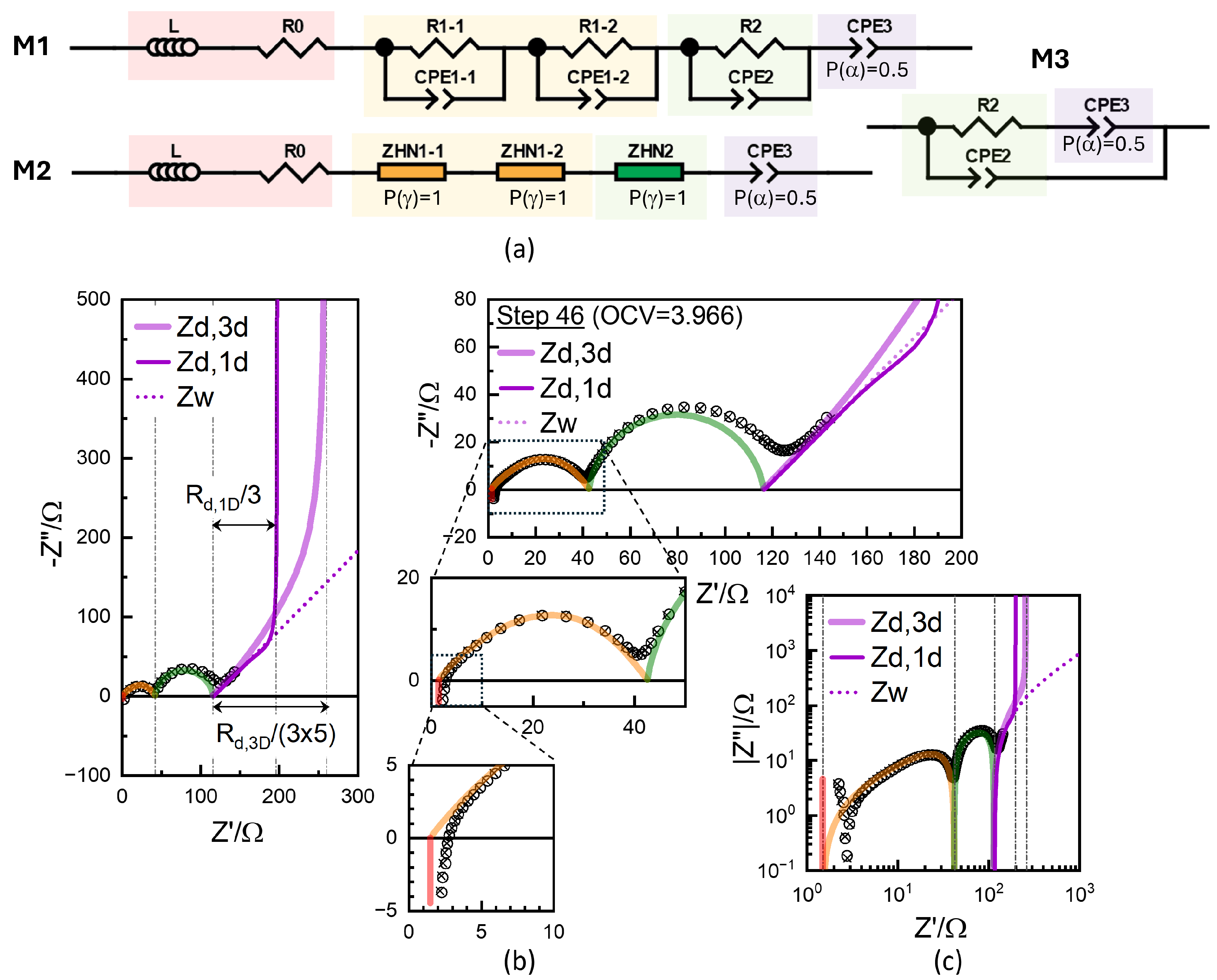
4.1. Equivalent Circuit Concept of Chemical Diffusivity

The kinetic and thermodynamic aspects in ${\tilde{D}}_{\mathrm{NMC}}$, Equation (2) or Equation (3), can expressed by the equivalent circuit elements of R and C [17]:

$${\tilde{D}}_{\mathrm{NMC}}=r^2/\left(R_{\mathrm{d}}{C}_{\mathrm{d}}\right)$$

(4)

or

$${\tilde{D}}_{\mathrm{NMC}}={({\sigma }_{{\mathrm{Li}}^{+}}^{-1}+{\sigma }_{\mathrm{e}}^{-1})}^{-1}/C_{\mathrm{d},\mathrm{volumetric}}$$

(5)

in terms of specific material properties: lithium ionic conductivity ${\sigma }_{{\mathrm{Li}}^{+}}$, electronic conductivity ${\sigma }_{\mathrm{e}}$, and volumetric chemical capacitance $C_{\mathrm{d},\mathrm{volumetric}}=C_{\mathrm{d}}(d_{\mathrm{NMC}}/m)$. Often the chemical diffusivity for lithiation is referred to as the lithium (ion) diffusivity. Ionic conductivity and self-diffusivity are related by the Nernst–Einstein relation. For the chemical diffusivity and self-diffusivity (or ionic conductivity), the thermodynamic factor or chemical capacitance needs to be considered, which can vary by several orders of magnitude.

The chemical (or diffusion) capacitance $C_{\mathrm{d}}$, $Q_{\mathrm{pulse}}/\Delta E_{\mathrm{s}}$, Figure 9c, was reciprocal to $\Delta E_{\mathrm{s}}$ in Figure 9b and exhibited a maximum of ca. 6 F around 3.75 V. Discharging points were shifted to the lower voltage but much smaller than $dQ/dV$ from the continuous charge–discharge cycles at 0.1 C, Figure 2b, where the asymmetry between charge and discharge was outlined. At high OCV, above 3.8 V, where the oxidation of Ni (Ni²⁺ → Ni³⁺ occurs, the smaller number of discharging steps than that of the charging steps corresponded to a larger $\Delta E_{\mathrm{s}}$ and a systematically smaller $C_{\mathrm{d}}$. The volumetric capacitance $C_{\mathrm{d},\mathrm{volumetric}}$ in Equation (5) and gravimetric capacitance were determined using the density of NMC622, $d_{\mathrm{NMC}}$, 4.98 g cm⁻³ and m = 3.02 mg, which are indicated by the additional y-axes in Figure 9c.

Using ${\tilde{D}}_{\mathrm{NMC}}$ from Figure 9a and $C_{\mathrm{d}}$ and $C_{\mathrm{d},\mathrm{volumetric}}$, Figure 9c, the diffusion resistance $R_{\mathrm{d}}$, Equation (4), and the lithium ionic conductivity ${\sigma }_{{\mathrm{Li}}^{+}}=(d_{\mathrm{NMC}}/m)(r^2/R_{\mathrm{d}})$, Equation (5), can be obtained, Figure 9d. $R_{\mathrm{d}}2054\Omega$ from $E_{\mathrm{t},\mathrm{ST}}$, for step 46 in Figure 7, is highlighted and corresponds to ${\sigma }_{{\mathrm{Li}}^{+}}=5.16\times {10}^{-8}$${\Omega }^{-1}$ cm⁻¹, assuming a much higher electronic conductivity ${\sigma }_{\mathrm{e}}$ in Equation (5).

The diffusion impedance in spherical geometry with the diffusivity as Equation (4) becomes [17,48]

$$Z_{\mathrm{d},3\mathrm{D}}\left(\omega \right)={\displaystyle \frac{1}{3}}{\displaystyle \frac{R_{\mathrm{d}}tanh\left(\sqrt{j\omega R_{\mathrm{d}}{C}_{\mathrm{d}}}\right)}{\sqrt{j\omega R_{\mathrm{d}}{C}_{\mathrm{d}}}-tanh\left(\sqrt{j\omega R_{\mathrm{d}}{C}_{\mathrm{d}}}\right)}}$$

(6)

of the magnitude $R_{\mathrm{d}}/(3\times 5)\approx 2054/15=137\Omega$, which is simulated in Figure 10b,c in thick purple line.

Figure 10. (a) Conventional equivalent circuit represented using CPE (MI) and Havriliak-Negami impedance function with P($\gamma$) =1 (M2) and Randles circuit variation (M3). Data for Step 46 (circles) along with the fitted results (crosses) using the equivalent circuit model M1 or M2 in different ranges (b) and in logarithmic scale (c). Diffusion impedances for one-dimension and three-dimension are simulated using $R_{\mathrm{d}}$ deduced from the low-frequency CPE with $\alpha =0.5$ for $C_{\mathrm{d}}$ from GITT (Figure 9c).

Chemical diffusivity has been shown to be reliably and straightforwardly obtained from diffusion impedance rather than from the time-domain analysis of long-term relaxation [50]. The measured impedance is often limited to the high-frequency response as

$$Z_{\mathrm{d},3\mathrm{D}}(\omega \to \infty )={\displaystyle \frac{1}{3}}\sqrt{{\displaystyle \frac{R_{\mathrm{d}}}{j\omega C_{\mathrm{d}}}}}.$$

(7)

The response can be modeled by a constant-phase element (CPE), briefly denoted as the “Q” element:

$$\begin{array}{cc}\hfill Z_{\mathrm{CPE}}\left(\omega \right)& ={\displaystyle \frac{1}{Q{\left(j\omega \right)}^{\alpha }}}\hfill \\ \hfill C_{\mathrm{CPE}}^{*}\left(\omega \right)& =Q{\left(j\omega \right)}^{\alpha -1}\hfill \end{array}$$

(8)

with $\alpha$ = 0.5. Therefore, from the $Q_{\mathrm{d},3\mathrm{D}}=3\sqrt{C_{\mathrm{d}}/R_{\mathrm{d}}}$ determined by EIS, from the simulated response shown as a dotted line in Figure 10b, denoted $Z_{\mathrm{W}}$, and $C_{\mathrm{d}}$ separately obtained from the OCV curve as 2.35 F, $R_{\mathrm{d}}$ can be estimated.

When the CPE with $\alpha$ = 0.5 represents the infinite Warburg response, $Z_{\mathrm{W}}$, it is also the high-frequency limit of the one-dimensional diffusion impedance for a flake or slab of l half-thickness, which corresponds to the surface-area-based chemical diffusivity estimation, Equation (2), as

$$Z_{\mathrm{d},1\mathrm{D}}\left(\omega \right)={\displaystyle \frac{R_{\mathrm{d}}coth\left(\sqrt{j\omega R_{\mathrm{d}}{C}_{\mathrm{d}}}\right)}{\sqrt{j\omega R_{\mathrm{d}}{C}_{\mathrm{d}}}}}$$

(9)

and the high-frequency limit becomes CPE as

$$Z_{\mathrm{d},1\mathrm{D}}(\omega \to \infty )=\sqrt{{\displaystyle \frac{R_{\mathrm{d}}}{j\omega C_{\mathrm{d}}}}}.$$

(10)

with $Q_{\mathrm{d},1\mathrm{D}}=\sqrt{C_{\mathrm{d}}/R_{\mathrm{d}}}$ Therefore, when the response is assumed to be one-dimensional diffusion, $R_{\mathrm{d},1\mathrm{D}}\approx 2054/9=228.2$ $\Omega$ is estimated either from the GITT and EIS. The one-dimensional diffusion impedance, $Z_{\mathrm{d},1\mathrm{D}}$, is simulated in Figure 10b in a thin purple line, with the limiting resistance being (1/3)$R_{\mathrm{d},1\mathrm{D}}\approx 76\Omega$. The limiting DC resistance, given by $Z_{\mathrm{d},3\mathrm{D}}^{\prime }(\omega \to 0)=R_{\mathrm{d}}/(3\times 5)$ and $Z_{\mathrm{d},1\mathrm{D}}^{\prime }(\omega \to 0)=R_{\mathrm{d}}/3$, is more clearly visible in the logarithmic scale in Figure 10c.

The simulated three-dimensional diffusion impedance exhibited an upward deviation from the high-frequency slope-one behavior, which appeared to describe the experimental data well (Figure 10b). The well-known finite-length Warburg diffusion for one-dimensional diffusion (Equation (9)) exhibited a downward deviation before the impedance diverged capacitively. Lower-frequency data were needed to compare the two diffusion impedance values and to assess the models more definitively. ${\sigma }_{{\mathrm{Li}}^{+}}$ and $R_{\mathrm{d}}$ are straightforwardly related in the case of a one-dimensional slab of thickness $2l$, where the diffusion length is l. Although defining conduction or conductivity becomes less intuitive for spherical (or cylindrical) geometry, Equation (4) can be generally used for the diffusion impedance for different diffusion geometries [17], while Equations (4) and (6) are defined for spherical diffusion, self-consistently, using “3$R_{\mathrm{d}}$” instead of $R_{\mathrm{d}}$ by Barsoukov et al. [48].

The analysis so far demonstrates the consistency between the GITT and EIS under the assumption of consecutive or series kinetic steps corresponding to $R_2$ and chemical diffusion in a solid state, as has been shown, e.g., in [34]. The slope-one behavior deviates at high frequencies due to overlapping capacitive effects, and the fitting of the diffusion impedance depends on the modeling of the $R_2$ response. Compared to the time-domain response, EIS provides detailed features of the $I_{\mathrm{p}}{R}_2$ contribution, separated by the distinguished R positions due to the large differences in the associated capacitance effects on a logarithmic scale, as shown in Figure 7f. In the following, the limitations of the conventional EIS analysis are first examined, setting the stage for a more detailed interpretation based on the physics-based three-rail TLM.

4.2. Conventional EIS Modeling

In determining ${\tilde{D}}_{\mathrm{NMC}}$ from the GITT analysis, the diffusion response is assumed to start at $E_2=I_{\mathrm{p}}{R}_2$, as shown in Figure 7a. The correlation between voltage transients in the GITT analysis and resistance values in EIS is presented on linear and logarithmic scales in (a) and (d) and (b) and (e), respectively. The short-time information corresponding to the position $R_0$ and $R_1$ is not visible in the time domain for the shortest interval of 0.1 s. Figure S14 illustrates an experiment in which the initial transient was measured at the minimum allowed interval of 20 μs, capturing the response corresponding to $R_1$. The impedance spectra of all Li-NMC622 and also Li-NMC811 coin cells investigated exhibited three distinguishable resistance positions, $R_0$, $R_1$, and $R_2$ (Figures S4–S13).

Although equivalent to such a time-domain response, EIS is superior in the deconvolution of the short-time or high-frequency responses. Moreover, EIS allows the effective modeling and analysis of multi-timescale processes in the frequency domain, whereas the analytic treatment of such processes is not trivial. Conventionally, in refs. [5,7,23,29,30,33,34,37,38,40,52,53], and as shown in Figure 10a, M1, the diffusion impedance is connected in series to the distinguishable arc-like impedance responses for $R_2$, which are modeled as the series network of the $RQ$ parallel connection of the impedance,

$$Z_{RQ}\left(\omega \right)={\displaystyle \frac{R}{1+RQ{\left(j\omega \right)}^{\alpha }}}$$

(11)

where Q represents a constant-phase element (CPE); see Equation (8).

The SOC-independent impedance R1 can be attributed to the contact impedance between the current collector and electrode mass interface [12,13]. The skewed arc can be more accurately fitted by two $\left(RQ\right)$s, which are denoted as R1-1, R1-2, CPE1-1, and CPE1-2. Another $\left(RQ\right)$ for R2, CPE-2, and CPE-3 with Q with $\alpha =0.5$, the short-time diffusion response, discussed above, are all connected in series in the M1 model. Together with R0, the ohmic resistance, and L for the lead wire inductance, the model simulation in cross symbols excellently describes the experimental data in circles; see Figure 10b. The parameters are shown in Table 1. (See also Figure S15 for full fit results including the errors in the parameters using ZView^®.) The same results can be obtained using any analysis software, provided that the magnitude (modulus) of the calculated or modeled impedance weighting is used in the least-squares optimization algorithm. (This corresponds to the “calc modulus” option in ZView^®.)

Table 1. Parameters for the modeling using CPEs and Havriliak–Negami impedance functions in Figure 10 and Figure 11. The symbol ∗ represents fixed parameters.

Parameter	M3	M1	Parameter	M2	M4
Chi-Sqr	7.87e-05	7.08e-05	Chi-Sqr	7.08e-05	9.24e-05
Sum-Sqr	1.18e-02	1.06e-02	Sum-Sqr	7.08e-05	1.40e-02
L	7.17e-07	7.17e-07	L	7.17e-07	7.28e-07
R0	1.51	1.51	R0	1.51	1.31
R1-1	32.57	30.10	ZHN1-1-R	30.10	39.14
CPE1-1-T	1.10e-04	1.12e-04	ZHN1-1-T	5.13e-05	1.27e-04
			ZHN1-1-P	1 *	0.614
CPE1-1-P	0.577	0.577	ZHN1-1-U	0.577	0.845
C1-1	1.77e-06	1.70e-06	C1-1
R1-2	9.42	11.13	ZHN1-2-R	11.13
CPE1-2-T	6.80e-06	8.10e-06	ZHN1-2-T	8.60e-05
			ZHN1-2-P	1 *
CPE1-2-P	1.028	0.995	ZHN1-2-U	0.995
C1-2	8.84e-06	7.73e-06	C1-2	7.73e-06	1.88e-06
R2	75.48	73.95	ZHN2-R	73.95	75.00
CPE2-T	1.88e-03	2.07e-03	ZHN2-T	1.23e-01	1.51e-01
			ZHN2-P	1	0.822
CPE2-P	0.902	0.894	ZHN2-U	0.894	0.948
C2	1.52e-03	1.66e-03	C2	1.66e-03	1.67e-03
CPE3-T	1.03e-01	9.86e-02	CPE3-T	9.86e-02	9.55e-02
CPE3-P	0.5 *	0.5 *	CPE3-P	0.5 *	0.5 *
$R_{\mathrm{d}}$	2000.2	2174.5	$R_{\mathrm{d}}$	2174.5	2320.7

As shown in the magnified partial spectra, the simulation of the R1 response in orange is a composite effect of CPE1-1-P (0.577) for a strongly depressed $\left(RQ\right)$ response, and CPE1-2-P (0.995) close to 1 for an ideal $\left(RC\right)$ semicircle. The overlapping of the two $\left(RQ\right)$s can be seen by the time constants ${\tau }_{RQ}={\omega }_{\mathrm{Peak}}$, which equivalently describe the $\left(RQ\right)$ response as

$$Z_{RQ}\left(\omega \right)={\displaystyle \frac{R}{1+{\left(j\omega {\tau }_{RQ}\right)}^{\alpha }}}$$

(12)

where ${\tau }_{RQ}^{\alpha }=RQ$. This equation corresponds to a special case of the Havriliak–Negami (HN) impedance with P (or $\gamma$) = 1 [48],

$$Z_{\mathrm{HN}}\left(\omega \right)={\displaystyle \frac{R}{{(1+{\left(j\omega {\tau }_{\mathrm{HN}}\right)}^{\beta })}^{\gamma }}}$$

(13)

which is available as model DE6 in ZView^® as shown in Figure S16. The fit results of the two models, M1 and M2, are exactly identical; see Table 1. The ${\tau }_{\mathrm{HN}}$ values clearly indicate the frequency range of the respective responses. ${\tau }_{\mathrm{HN}}$ for R1-1 and R1-2 are 5.13 × 10⁻⁵ s and 8.60 × 10⁻⁵ s, very close, which are much smaller than 0.123 s for the R2 response. With arbitrarily adjustable exponents P($\gamma$), not fixed to one, somewhat different R1 and R2 values result; see Figure 11 and Figure S17 and Table 1.

Figure 11. (a) Impedance data for step 46 (circles) along with the fitted results (crosses) using the Havriliak–Negami impedance functions (Equation (13)) with free exponents $\gamma$ and $\beta$, in M4 model (top) Results with Havariliak–Negami capacitance function (Equation (18)) for R1 using M5 model are shown in (b). The model provides an R0 close to the intercept and directly represents the capacitance effects in the raw data.

The components R2, CPE2, and CPE3 can be connected in a Randle’s circuit configuration [9,55], M3, [4], resulting in slightly changed parameters; see Table 1 and Figure S18. CPE1-2-P becomes larger than one. The excellent goodness of fit in conventional modeling primarily arises from the inclusion of multiple CPEs with adjustable exponents ($\alpha$), denoted as CPE-P in ZView^®. Values larger than 1 and much smaller than 0.5 have been reported. Fit results should not be considered more scientific or accurate than direct readings unless the employed fit models are properly justified. From the CPE-3 with $\alpha =0.5$ fixed, $Q_{\mathrm{d},3\mathrm{D}}$ was obtained as 0.0986 (M1,M2), 0.1028 (M3), and 0.0955 (M4) F·s^−0.5, from which $R_{\mathrm{d}}$ was evaluated as 2174, 2000, and 2320 $\Omega$ (Table 1) comparable to the 2054 $\Omega$ from the GITT short-time analysis.

For either model, the fit results, represented by cross symbols, demonstrated that the model accurately reproduced the experimental data in the circles. However, the fit quality did not necessarily support the scientific significance, as there is no special physics behind the conventional $\left(RQ\right)$ modeling ($Z_{\mathrm{HN}}$ with P($\gamma$) = 1) or $Z_{\mathrm{HN}}$ with arbitrary P($\gamma$) and U($\beta$) in Equation (13). The R values, often the only ones considered among the fit parameters, depend on the models. In Figure 10, R0 values fitted are shown to be substantially smaller than the x-axis intercept, as they are the extrapolation from the CPE response with the exponents $\propto {\omega }^{\alpha }$ or $\propto {\omega }^{\gamma \beta }$ optimized using the least-squares fitting. For ZHN1, the high-frequency slope $\gamma \beta =0.614\times 0.845=0.52$, close to 0.5. The inset shows that ohmic resistance R0 is further left from the x-axis intercept, since the L element shifts the intercept close to that of the experimental data. Without a proper justification, $\left(RQ\right)$ or $Z_{\mathrm{HN}}$ modeling can lead to artefactual errors in the extracted parameters.

The ideal theoretical form of these models can be $R\left(RC\right)\left(RC\right)$, where the R and C represent well-defined physical quantities. The absolute magnitude of the capacitance in an $R\left(RC\right)$ circuit can be directly obtained by subtracting the series resistance, thereby reducing the system to an $RC$ circuit. Figure 7f shows the absolute C effects resulting from the data manipulation. They should be comparable to the effective C estimated from the peak frequency, ${\omega }_{\max }=1/{\tau }_{RQ}$, assuming that ${\tau }_{RQ}={\tau }_{RC}$, which is directly parameterized in the $Z_{\mathrm{HN}}$ model with P($\gamma$) = 1. For the negatively skewed impedance arcs with P($\gamma$) < 1, $\tau ={\omega }_{\mathrm{Peak}}^{-1}$, smaller than ${\tau }_{\mathrm{HN}}$ [67], can be used to evaluate the effective capacitance values as presented in Table 1.

Thus, the obtained C2 is comparable to the capacitance plateau around 2 × 10⁻³ F F, denoted by $C_{\mathrm{dl}}$. C1 or C1-1 corresponds to the kink position around 2 × 10⁻⁶ F, indicated as $\Delta C_{\mathrm{HN}}$, when $R_0$, read from the x-axis intercept, is subtracted. In fact, the capacitance effects associated with the R1 response are distributed from around 3 × 10⁻⁷ F, denoted by “$C_{\mathrm{B}0}$”, which is not parameterized in the present modeling; see Figure 10 and Figure 11.

The R and C parameters read from the raw data may not be considered less accurate than the modeling using CPE or Havriliak–Negami impedance functions using arbitrarily adjusted frequency power exponents. EIS modeling of well-defined R and C elements connected in a physics-based manner can be meaningful and powerful in general. This is shown in the following.

4.3. Physics-Based EIS Modeling

The physics-based three-rail TLM and parameters for the step 46 EIS data are illustrated in Figure 12. The TLM for porous electrodes should be used when the electrolyte resistance in the tortuous pore network, where active material spheres are dispersed, is not negligible. The solid-state diffusion impedance, $Z_{\mathrm{d},3\mathrm{D}}$, as well as the charge transfer resistance at the electrolyte/solid interface, is distributed and modulated by the non-negligible pore resistance. Thus, the diffusion process is not connected in an overall series configuration, in contrast to the assumption made in conventional GITT and EIS analyses discussed in the preceding section. Furthermore, since the transference number of active Li⁺ ions in the electrolyte, $t_{+}$, is typically around 0.3, ambipolar diffusion in the pore liquid phase occurs alongside such solid-state diffusion. The apparent solid-state chemical diffusivity estimated by the GITT, without accounting for concurrent liquid-phase diffusion, can underestimate the true value, as demonstrated by comparisons between the GITT analysis and DFN model simulations [25,28,41].

Figure 12. Three-rail TLM model for an NMC-Li cell (adapted from [12]), along with the parameters used for the simulations in Figure 13.

$R_{\mathrm{d}}$ was adjusted (or fitted) to 514.2 $\Omega$, which was substantially smaller than 2054 $\Omega$ from the GITT analysis (Figure 9d) or similar values from EIS assuming series-connected diffusion impedance (Figure 10 and Figure 11) (Table 1) and that of the “Bisquert” model in to be explained below. Chemical diffusivity correspondingly increased to 5.32$\times$10⁻¹¹ cm²s⁻¹ (Figure 9a) from 1.24$\times$10⁻¹¹ cm²s⁻¹, by about four times.

With the non-negligible resistance of the electrolyte in the tortuous pore network, $R_{\mathrm{por}}$, indicated in the green part of the TLM in Figure 12, the impedance of the TLM becomes

$$Z_{\mathrm{Barsoukov}}\left(\omega \right)=\sqrt{{\displaystyle \frac{R_{\mathrm{por}}(R_{\mathrm{ct}}+Z_{\mathrm{d},3\mathrm{D}})}{1+j\omega (R_{\mathrm{ct}}+Z_{\mathrm{d},3\mathrm{D}})C_{\mathrm{dl}}}}}coth\sqrt{{\displaystyle \frac{R_{\mathrm{por}}}{(R_{\mathrm{ct}}+Z_{\mathrm{d},3\mathrm{D}})}}+j\omega R_{\mathrm{por}}{C}_{\mathrm{dl}}}$$

(14)

In this work, the model is referred to as the Barsoukov TLM in recognition of his extensive contributions to its description and interpretation for the different diffusion geometries [48,68,69]. The Barsoukov models are available in MEISP [70], FitmyEIS [71], or ZView^® (DX-28). When $R_{\mathrm{por}}$ is negligibly small, Randle’s circuit of $R_{\mathrm{ct}}$ and $Z_{\mathrm{d}}$ in series, which is in parallel with $C_{\mathrm{dl}}$, distributed in a transmission line network, becomes equivalent to the circuits in Figure 10. The fully analytical Barsoukov TLM becomes equivalent to the impedance response described by the Newman model when diffusion in the solution phase is neglected—a condition also known as the single-particle model (SPM) [72].

The high-frequency response of the Barsoukov TLM, which corresponds to the condition $Z_{\mathrm{d},3\mathrm{D}}=0$ in Equation (14), can be described as

$$Z_{\mathrm{Bisquert}}\left(\omega \right)=\sqrt{{\displaystyle \frac{R_{\mathrm{por}}{R}_{\mathrm{ct}}}{1+j\omega R_{\mathrm{ct}}{C}_{\mathrm{dl}}}}}coth\sqrt{{\displaystyle \frac{R_{\mathrm{por}}}{R_{\mathrm{ct}}}}+j\omega R_{\mathrm{por}}{C}_{\mathrm{dl}}}$$

(15)

The model represents the distributed electrode reaction for the exchange currents in fuel cells, electrolyzers, and other electrochemical energy systems. This model is known as the Bisquert TLM, in recognition of his extensive contributions (e.g., [73]). The battery impedance has been described using the Bisquert TLM to model the high-frequency response or with the solid-state diffusion impedance connected in series with the Bisquert TLM [31,74,75,76], which can be compared to the Barsoukov-type formulation.

In the Barsoukov (and Bisquert) model, the electrolyte resistance in the separator, $R_{\mathrm{sep}}$, and in the pores, $R_{\mathrm{por}}$, is treated as a pure resistor. In contrast, Newman’s battery model explicitly accounts for diffusion in the electrolyte, arising from the buildup of a salt concentration gradient due to the accumulation of unused anions—here, ${\mathrm{PF}}_6^{-}$—through which Li⁺ transport occurs predominantly by diffusion rather than drift. This process is governed by the effective solution-phase diffusivity, ${\tilde{D}}_{\mathrm{liq}}$ [58]. The evolution of this concentration gradient in the liquid phase is central to Newman’s model and plays a key role in simulating battery performance, as implemented in frameworks such as PyBaMM [77].

Impedance studies based on Newman’s model [64,65,66] have shown that the chemical diffusivity of the active material cannot be accurately estimated from the low-frequency response due to overlapping effects from the solution-phase diffusion. Although the liquid-phase diffusivity (${10}^{-6}{\mathrm{cm}}^2{\mathrm{s}}^{-1}$) is several orders of magnitude higher than the solid-state diffusivity (${10}^{-11}{\mathrm{cm}}^2{\mathrm{s}}^{-1}$), the effective diffusion lengths of the porous electrodes and separator, $l_{\mathrm{por}}^{\tau }$ and $l_{\mathrm{sep}}^{\tau }$, can be three to five times their nominal thicknesses—$l_{\mathrm{por}}=117\mathsf{\mu }\mathrm{m}$ and $l_{\mathrm{sep}}=25\mathsf{\mu }\mathrm{m}$—due to the tortuosity. These effective lengths are much larger than the active particle radius of $2.54\mathsf{\mu }\mathrm{m}$, through which solid-state diffusion occurs. Since the characteristic diffusion relaxation time scales with the square of the length divided by diffusivity, the time constants for liquid- and solid-phase diffusion can become comparable, despite the large difference in intrinsic diffusivities [65].

In Newman’s concentrated solution theory for lithium-ion battery electrolytes, the kinetic interactions among solvated cations, solvated anions, and large solvent molecules govern the diffusivity ($D_{\mathrm{liq}}$), ionic conductivity ($\kappa$), and transference number ($t_{+}$). However, most practical implementations of the Newman model do not account for the full set of kinetic interaction parameters. Instead, $D_{\mathrm{liq}}$, $\kappa$, and $t_{+}$ are typically treated as independently variables, despite their interdependence through the interaction coefficients which are not explicitly considered [64,65,66]. Newman and co-authors reported the impedance response in the absence of solution-phase diffusion [72], which corresponds to the Barsoukov transmission line model (TLM).

When the Nernst–Planck flux’s behavior of the binary electrolyte, Li⁺ and ${\mathrm{PF}}_6^{-}$, is assumed, ambipolar diffusion occurs in a manner similar to ${\tilde{D}}_{\mathrm{NMC}}$ for lithium intercalation in the active mixed conductor material (Equation (5)), given by:

$${\tilde{D}}_{\mathrm{liq}}={\displaystyle \frac{{({\kappa }_{+}^{-1}+{\kappa }_{-}^{-1})}^{-1}}{C_{\mathrm{liq}}}}$$

(16)

where $\kappa ={\kappa }_{+}+{\kappa }_{-}$ represents the liquid electrolyte conductivity. The transference number is given by:

$$t_{+}={\displaystyle \frac{{\kappa }_{+}}{{\kappa }_{+}+{\kappa }_{-}}}$$

(17)

which can be represented by the equivalent circuits in the lower blue box in Figure 12, indicated as Nernst–Planck TLM.

The Nernst–Planck model for lithium-ion batteries (LIBs) appears to be approximately and self-consistently applicable in many cases. Commonly employed transference number values, such as $t_{+}=0.3$, are often determined using the Bruce–Vincent method [78], which is itself based on the Nernst–Planck framework. However, as described by the concentrated solution theory, kinetic interactions between ions and solvent molecules can result in $t_{+}$ values that approach zero or even become negative [79]. Newman’s concentrated solution theory reduces to the Nernst–Planck model in the dilute-solution limit, where such interactions are negligible [58]. The Nernst–Planck model assumes charge neutrality between the two ionic carriers, and non-ideal thermodynamic behavior can still be incorporated through a concentration term $C_{\mathrm{liq}}$, modified from the ideal case—analogous to how the differential capacitance $C_{\mathrm{d}}$ is defined in terms of lithium activity via the open-circuit voltage (OCV) [80,81].

Moškon et al. [12,13] simplified more rigorous three-dimensional networks—also reported by Siroma et al. [82]—into the two-dimensional three-rail TLM shown in Figure 12. In this model, the porous electrode structure described by the Barsoukov TLM is combined with a Nernst–Planck-based TLM for the electrolyte. The electrolyte TLM is extended through the separator region, and further into the counter electrode in full-cell configurations. The distributed R and C elements vary with the porosity and tortuosity in each respective region.

In the present work, the transference number $t_{+}$ was applied consistently to the liquid electrolyte across different regions, which is physically reasonable and simplifies the parameter adjustment. In Bruce’s method, the DC limiting current of lithium symmetric cells was measured, and the non-negligible interfacial resistance was determined by EIS and subtracted from the total resistance [78,83]. This principle can be implemented more rigorously and practically by measuring electrochemical impedance spectra down to low frequencies near the DC limit, without resorting to DC polarization techniques [16,18]. Values around 0.3 have been reported for $1\mathrm{M}$ LiPF₆ in EC:DMC (1:1 v/v) [16,83].

The response of the three-rail TLM and/or inhomogeneous TLM across electrodes and the separator needs to be calculated numerically by putting hundreds of the distributed circuits in each region or in meshes [12,13,84]. The Python code used in this work was shared in June 2023 for this work and is now public in the supplementary information of [14].

Some of the parameters were determined by fitting the analytical part of the model, such as the Barsoukov TLM for NMC622 and the $RC$ element for the lithium electrode, and were then refined numerically. The complete set of parameters obtained through this process is summarized in Table 2 and illustrated in Figure 12. The corresponding simulation results are shown in Figure 13a,b, with impedance portions labeled a to f, following the notation used in refs. [12,13].

Table 2. Parameters for the 3-rail TLM for the $t_{+}=0.3$, Barsoukov, and Bisquert models. A dash (–) indicates that the value is the same as in the 3-rail TLM unless otherwise noted. ${\tilde{D}}_{\mathrm{NMC}}$ was estimated from $R_{\mathrm{d}}$ and $R_{\mathrm{d}}$ with $r=0.254$ μm (Equation (3)).

Parameter	3-Rail TLM	Barsoukov	Bisquert
T/°C	30	–	–
m/g	3.02e-03	–	–
d/g cm−3	4.98	–	–
r/cm	2.535e-04	–	–
$E_{\mathrm{OCV}}$/V	3.966	–	–
$C_{\mathrm{d}}$	2.35	–	–
$t_{+}$	0.3	1	n.a.
$\gamma$	1.855	–	–
$\alpha$	0.444	–	–
L	2.49e-07	–	–
$C_{\mathrm{B}}0$	2.91e-06	–	–
$\Delta C_{\mathrm{HN}}$	1.79e-05	–	–
${\tau }_{\mathrm{HN}}$	7.05e-05	–	–
$C_{\mathrm{Li}}$	2.69e-03	–	–
$C_{\mathrm{dl}}$	8.18e-03	8.07e-03	1.13e-02
$C_{\mathrm{sep}}$	0.813	n.a.	n.a.
$C_{\mathrm{por}}$	0.593	n.a.	n.a.
$R_{\mathrm{sep}}$ (a)	2.2	–	–
$R_{\mathrm{A}}$ (b)	36.5	–	–
$R_{\mathrm{Li}}$	42.2	–	–
$R_{\mathrm{por}}$	50.3	–	–
$R_{\mathrm{ct}}$	22.7	22.6	19.9
$R_{\mathrm{d}}$	514.2	1865.3	2212.8
c	37.4	37.4	34.4
d	62.2	n.a.	n.a.
e	5.1	n.a.	n.a.
$c+R_{\mathrm{Li}}$	79.6	79.6	76.6
$d+e-c$	29.9	n.a.	n.a.
f	50.7	126.4	147.5
a	2.2	–	–
$a+b$	38.7	–	–
$a+b+R_{\mathrm{Li}}$	80.9	–	–
$a+b+R_{\mathrm{Li}}+c$	118.3	118.2	115.3
$a+b+R_{\mathrm{Li}}+c+e$	123.4	n.a.	n.a.
$a+b+R_{\mathrm{Li}}+d+e$	148.2	n.a.	n.a.
$R_{\mathrm{dc}}$	198.8	244.6	262.8
${\tilde{D}}_{\mathrm{NMC}}$/cm2s−1	5.32e-11	1.47e-11	1.24e-11
$C_{\mathrm{d}},\mathrm{gra}$/kF g−1	0.778	–	–
$C_{\mathrm{d}},\mathrm{vol}/\mathrm{kF}{\mathrm{cm}}^{-3}$	3.875	–	–
${\sigma }_{{\mathrm{Li}}^{+}}$/${\Omega }^{-1}$cm−1	2.063-07	5.68e-8	4.79e-8
$log(\sigma /{\Omega }^{-1}$cm−1)	−6.69	−7.25	−7.32

Figure 13. Three-rail TLM simulation in the impedance plane with an imaginary Bode plot (a), impedance plane plots in a wider range (b), real impedance Bode plot (c), and capacitance Bode plot (d). Limiting resistance and capacitance values of the segments (Table 2) indicated by the color. See the text for details.

The R0 and R1 responses can be attributed to the electrolyte’s ohmic resistance, $R_{\mathrm{sep}}$ (assuming negligible electronic resistance in the electrode at the top rail), and the contact impedance between the current collector (aluminum) and the NMC electrode mass, $R_{\mathrm{A}}$, as shown in Figure 12. These correspond to the impedance portions labeled a and b, respectively, in Figure 13, following the notation used in refs. [12,13].

The resistance values directly obtained from the spectra, $R_0=\mathrm{R}0$ and $R_1=\mathrm{R}0+\mathrm{R}1$, are shown to be independent of the state of charge (SOC), as illustrated in Figure 8. A similar trend was observed for the thin NMC electrode (20 μm) in Figure S9 [4]. In contrast, for other NMC622 and NMC811 cells, $R_1$ increased at a low SOC, following a trend similar to that of $R_2$, as shown in Figures S5–S8 and S10–S13, suggesting a common origin contributing to $R_1$. These $R_1$ values were substantially larger than those in Figure 8 even at high OCV.

The skewed or overlapped R1 response was described using either two $\left(RQ\right)$ elements or a single $Z_{\mathrm{HN}}$ element with two adjusted exponents, as shown in Figure 10 (Figure S15) and Figure 11 (Figure S17) in the preceding section. In contrast to dividing $R_1$ artificially into components such as R1-1 and R1-2, the Havriliak–Negami (HN) capacitance function enables a direct description using a single resistance parameter $R_{\mathrm{A}}$, along with the characteristic capacitances $C_{\mathrm{B}}0$ and $\Delta C_{\mathrm{HN}}$ evident in the raw data:

$$C_{\mathrm{HN}}^{*}\left(\omega \right)=C_{\mathrm{B}}0+{\displaystyle \frac{\Delta C_{\mathrm{HN}}}{{[1+{\left(j\omega {\tau }_{\mathrm{HN}}\right)}^{\beta }]}^{\gamma }}}$$

(18)

This formulation represents a modified Debye response introduced by Havriliak and Negami [85], as illustrated in Figure 11b.

In conjunction with other parameters from the Barsoukov TLM analysis (Figures S19 and S20), the fitted exponents $\gamma =1.855$ and $\beta =0.444$ describe a positively skewed capacitance arc (Figure S21). These values are close to the widely used case of $\gamma =2$ and $\beta =0.5$, for which the product $\beta \gamma =1$ [86,87,88]. The impact of different exponent values on the capacitance spectra is illustrated in Figure S21. This distributed capacitance is attributed to lateral inhomogeneity at the electrode–current collector interface. The well-defined limiting capacitance, $C_{\mathrm{HN}}$, produces a nearly semicircular arc at low frequencies in the simulation (Figure 14a), in contrast to the more depressed semicircle resulting from the conventional CPE fit with $P=0.57657$ in CPE1-1 (Figure 10b). The high-frequency intercept $R_0$, denoted $R_{\mathrm{sep}}$ (or a in Refs. [12,13]), lies closer to the x-axis intercept of the raw data when using the TLM model, compared to the conventional CPE or ZHN fittings (cf. Figure 10 and Figure 11a,b).

Figure 14. Barsoukov TLM simulation or 3-rail TLM with $t_{+}=1$ in the impedance plane (a), impedance plane plots in a wider range (b), real impedance Bode plot (c), and capacitance Bode plot (d). Limiting resistance and capacitance values of the segments (Table 2) indicated by the color.

The $R_2$ or R2 of NMC622 cells increases at a low SOC below 3.7 V (Figure 8 and Fugures S4–S6, and S9), while it remains largely independent in the high OCV region. NMC811, on the other hand, shows an increase in $R_2$ at both low and high OCVs, with a minimum around 3.8 V (Figure S7), as also reported in [12]. The associated capacitance, $C_{\mathrm{dl}}$, as indicated in Figure 7f, by subtracting $R_1$, was evaluated using the relaxation time of the $\left(RQ\right)$ and $Z_{\mathrm{HN}}$ models as 0.0015–0.0017 F; see Table 1.

The SOC dependence is attributed to the $R_{\mathrm{ct}}$ of the NMC electrode. Although not distinguishable, the response R2 also includes the response of the lithium electrode. The impedance behavior of the lithium electrode can be qualitatively and quantitatively diverse due to SEI formation and dendrite growth [84]. A non-negligible contribution has been confirmed [16]. It is a fundamental and critical limitation in the widely used laboratory coin cells for studying electrode properties. Therefore, the ideal model parameters for porous electrodes as above were assumed for the NMC electrode, and the Li electrode response was simply modeled by $\left(R_{\mathrm{Li}}{C}_{\mathrm{Li}}\right)$ as for the ideally planar electrode. The Bisquert TLM response of NMC622 and the lithium electrode response contributed to R2. The ZView^® DX-28 Barouskov model with $R_{\mathrm{d}}$ = 0 (Figure S23, left) or DX-22 Bisquert model can also be applied (Figure S23, right). The impedance magnitude of $Z_{\mathrm{Bisquert}}\left(\omega \right)$ is given by:

$$c=Z_{\mathrm{Bisquert}}(\omega \to 0)=\sqrt{R_{\mathrm{por}}{R}_{\mathrm{ct}}}coth\sqrt{{\displaystyle \frac{R_{\mathrm{por}}}{R_{\mathrm{ct}}}}}$$

(19)

and thus R2 corresponds to $c+R_{\mathrm{Li}}$.

The fact that the five parameters, $R_{\mathrm{Li}}$, $C_{\mathrm{Li}}$, $R_{\mathrm{por}}$, $R_{\mathrm{ct}}$, and $C_{\mathrm{dl}}$, describe the skewed arc of the R2 response very nicely; similarly, the $Z_{\mathrm{HN}}$ model with the four parameters in Figure 11 does not justify the models nor the parameters. The parameters of contact impedance, lithium electrode impedance, $R_{\mathrm{Li}}$, $C_{\mathrm{Li}}$, and $R_{\mathrm{por}}$ are fixed from a Barsoukov TLM analysis, and $R_{\mathrm{ct}}$ and $C_{\mathrm{dl}}$ are slightly and $R_{\mathrm{d}}$ substantially adjusted upon the introduction of $t_{+}$, $C_{\mathrm{por}}$, and $C_{\mathrm{sep}}$ of the three-rail TLM.

The upper spectrum in black displays the separated ($R_{\mathrm{Li}}{C}_{\mathrm{Li}}$) semicircle and Bisquert TLM response of the magnitude c, Equation (19), by arbitrarily varying the associated capacitances as $C_{\mathrm{Li}}\ll C_{\mathrm{dl}}$ to show the magnitude of c and $R_{\mathrm{Li}}$ in the fit results.

The $R_{\mathrm{por}}$ value determines d:

$$d=\sqrt{(R_{\mathrm{por}}/t_{+})R_{\mathrm{ct}}}coth\sqrt{(R_{\mathrm{por}}/t_{+})/R_{\mathrm{ct}}}.$$

(20)

where $R_{\mathrm{por}}/t_{+}$ with $t_{+}=0.3$ representing the Li⁺ transport in the pore electrolyte of the electrode and replaces $R_{\mathrm{por}}$ in Equation (19). The parameter $R_{\mathrm{por}}$ for R2 or c from the Bisquert response further determines the magnitude $d-c$ of the lower frequency response, which is determined by $t_{+}$ assumed to be 0.3.

The e portion is similarly and directly related to $R_{\mathrm{sep}}$ or a as

$$e={\displaystyle \frac{R_{\mathrm{sep}}}{t_{+}}}-R_{\mathrm{sep}}=a\left({\displaystyle \frac{1}{t_{+}}}-1\right)=a{\displaystyle \frac{t_{-}}{t_{+}}}$$

(21)

It is to be noted that e depends on the estimation of $R_{\mathrm{sep}}$ or a, which is shown to substantially vary in percentages with the modeling; see Figure 10 and Figure 11. When substantial wire resistance is included in a, which is likely for large-area commercial cells, the portion e will also be incorrectly estimated for the given $t_{+}$.

In the upper black spectrum, the portions e and $d-c$ were separated by arbitrarily varying the C parameters as $C_{\mathrm{sep}}\ll C_{\mathrm{por}}$. $C_{\mathrm{sep}}$ and $C_{\mathrm{por}}$ are volumetric and thus increase with the amount of liquid for the given liquid concentration. The adjusted values 0.813 and 0.593 F were comparable, while $R_{\mathrm{sep}}\ll R_{\mathrm{por}}$. The impedance responses overlapped, as shown by the blue spectrum in the magnitude of $d-c+e$, which was simulated with $C_{\mathrm{HN}}^{*}$, $C_{\mathrm{dl}}$, and $R_{\mathrm{d}}$ equal to zero. The response overlapped with the R2 response from the high-frequency side and with solid-state diffusion from the low-frequency side, which is shown in the imaginary Bode plot in Figure 13b.

The segment f was simulated with all capacitance parameters equal to zero except $C_{\mathrm{d}}$ in the three-rail TLM, as shown in Figure 12. It should be noted that f does not represent the diffusion impedance, $Z_{\mathrm{d},3\mathrm{D}}$, when connected in series to the segments $a+b+d+e+R_{\mathrm{Li}}$, Figure 10, Figure 11 and Figure 15. With d, Equation (20), the f portion constitutes the overall dc resistance of the three-rail TLM for NMC:

$$Z_{\mathrm{NMC}}^{\prime }(\omega \approx 0)=d+f=R_{\mathrm{ct}}+{\displaystyle \frac{1}{3}}{\displaystyle \frac{R_{\mathrm{por}}}{t_{+}}}+{\displaystyle \frac{1}{3}}{\displaystyle \frac{R_{\mathrm{d}}}{5}}$$

(22)

The overall resistance of the three-rail TLM becomes the simple addition of $R_{\mathrm{ct}}$, the dc resistance of the TLM of the cationic rail with an eventually blocked terminal, $(1/3)(R_{\mathrm{por}}/t_{+})$, and the resistance of the spherical diffusion impedance, $(1/3)(R_{\mathrm{d}}/5)$ (Equation (6)). It should be noted that the respective terms are well defined individually but do not correspond to any distinguished or distinguishable components in the EIS indicated in Figure 13, c, $d-c$, and f.

$$f=R_{\mathrm{ct}}+{\displaystyle \frac{1}{3}}{\displaystyle \frac{R_{\mathrm{por}}}{t_{+}}}+{\displaystyle \frac{1}{3}}{\displaystyle \frac{R_{\mathrm{d}}}{5}}-\sqrt{(R_{\mathrm{por}}/t_{+})R_{\mathrm{ct}}}coth\sqrt{(R_{\mathrm{por}}/t_{+})/R_{\mathrm{ct}}}$$

(23)

f becomes a purely diffusion impedance, $R_{\mathrm{d}}/15$, when $R_{\mathrm{por}}=0$, i.e., when there is no TLM. f becomes much larger than $R_{\mathrm{d}}/15$ with a larger $R_{\mathrm{por}}$ and smaller $t_{+}$. Applications of physics-based EIS and deconvolution of the parameters are absolutely needed to obtain the parameters of physical significance, $R_{\mathrm{ct}}$, $R_{\mathrm{por}}$, and $R_{\mathrm{d}}$. In Table 2, the parameter values, the segments, and the cumulated segments indicated in Figure 13 are presented.

Figure 15. Simulation with the Bisquert TLM in series with the diffusion impedance, Bisquert-$Z_{\mathrm{d},3\mathrm{D}}$, in the impedance plane (a), impedance plane plots in a wider range (b), real impedance Bode plot (c), and capacitance Bode plot (d). Limiting resistance and capacitance values of the segments (Table 2) indicated by the color.

The parameters corresponding to the responses R0, R1, and R2 of the three-rail TLM analysis were determined from Barsoukov TLM; see Figures S19 and S20 and Table 2. The Barsoukov TLM corresponds to the three-rail TLM when $t_{+}=1$ or for very high $D_{\mathrm{liq}}$ by neglecting small $C_{\mathrm{por}}$ and $C_{\mathrm{sep}}$ in Equation (16), reducing to the two-rail TLM.

The impedance of any two-rail TLM with four different terminals can be analytically expressed [89] and thus can be fitted by the least-squares optimization. The separator part, now simply $R_{\mathrm{sep}}$, the lithium electrode response, ($R_{\mathrm{Li}}{C}_{\mathrm{Li}})$, and the contact impedance of the magnitude R1 or $R_{\mathrm{A}}$ can all be connected in series and fitted together. The fit results using ZView^® and a custom Python script developed in the laboratory are given in Figures S15 and S16, respectively, which are identical except for one caution. Between the two programs, $R_{\mathrm{d}}$ values differed by the factor three, since the definition of the spherical diffusion impedance and chemical diffusion from Barsoukov [48] differed by a factor of three in $R_{\mathrm{d}}$ from the present work in Equations (4) and (6). The present definition may be preferred as the chemical diffusion can be defined with the same $R_{\mathrm{d}}$ for different diffusion geometries.

These parameters were used for the three-rail TLM simulation discussed above, with a minor adjustment of $R_{\mathrm{ct}}$ and $C_{\mathrm{dl}}$, the response of which overlap the response of Nernst–Planck TLM described by $C_{\mathrm{por}}$ and $C_{\mathrm{sep}}$, and $t_{+}$ Since $R_{\mathrm{ct}}$ was similar and $R_{\mathrm{por}}$ and $R_{\mathrm{sep}}$ were the same, the segments $a+b+c+R_{\mathrm{Li}}$ were almost the same in Figure 13 and Figure 14. Although the fitted $R_{\mathrm{d}}$ for the Barsoukov TLM was 1865.3 $\Omega$, it was adjusted to 514.2 $\Omega$ for the three-rail TLM. This parameter adjustment resulted from the contribution of the liquid-phase diffusion to the experimental low-frequency response. The limiting resistance of the diffusion impedance, $R_{\mathrm{d}}/15$, became 124.4 $\Omega$ and 34.3 $\Omega$, respectively. As the diffusion impedance $Z_{\mathrm{d},3\mathrm{D}}$ was distributed within the TLM, the f segment became 126.4 $\Omega$ via Equation (23) for the Barsoukov TLM ($t_{+}=1$), and 50.6 $\Omega$ for the three-rail TLM with $t_{+}=0.3$. For the three-rail TLM with $t_{+}=0.3$, the additional term $d+e-c=29.9\Omega$ from the diffusion of the liquid phase in the pores of the electrode and in the pores of the separator contributed to $R_{\mathrm{dc}}$ by 45.8 $\Omega$. Even then, the substantially reduced contribution of $R_{\mathrm{d}}$ in the three-rail TLM resulted in a smaller overall dc resistance, 198.8 $\Omega$ vs. 244.6 $\Omega$.

The GITT short-time analysis and conventional EIS modeling assume the diffusion process in series with the reaction steps. Similarly to the analysis in the previous section, the Bisquert TLM, which is the Barsoukov TLM with $Z_{\mathrm{d},3\mathrm{D}}$ = 0, was used for the contribution in R2, and $Z_{\mathrm{d},3\mathrm{D}}$ was connected in series. With all other parameters fixed from the Barsoukov TLM fitting, $R_{\mathrm{ct}}$, $C_{\mathrm{dl}}$, and $R_{\mathrm{d}}$ were fitted using the Python code (Figure S22) and an $R_{\mathrm{d}}$ of 2212.5 $\Omega$ as in Table 2, which was comparable to the previous EIS analysis shown in Figure 10 and Figure 11 and Table 1. The model fitting was performed using ZView^® DX-28 or DX-22 for the Bisquert TLM and DX-28 for spherical diffusion, as shown in Figure S23, by setting the unused parameters to zero. The impedance characteristics are presented in Figure 15. Now, the segment f corresponds to $R_{\mathrm{d}}/15=147.5\Omega$, which is larger than the f of the Barsoukov TLM with $R_{\mathrm{d}}$ estimated as 1865.3 $\Omega$. Unlike the Barsoukov TLM and the three-rail TLM, $R_{\mathrm{ct}}$ is notably reduced, the resulting c and f segment boundary notably deviating from the $R_2$ position. For the assumed ideal TLM and the ideal $RC$ response for the R2 response, the uncorrelated diffusion impedance must describe the overlapped range.

It was shown that the physics-based three-rail TLM considering the liquid-phase diffusion could provide the correct solid-state chemical diffusivity, which could be substantially higher (around a factor of four) than when obtained from the GITT and the equivalent conventional EIS analysis, where the solid-state diffusion process was considered a series process after the electrode reaction. This is in line with previous reports on the effects of liquid-phase diffusion when the analysis of the DFN model was compared with the GITT analysis [25,28,41]. The solid-state diffusivity estimated via the Newman model, including the liquid-phase solution, was shown to be larger than that of the GITT kinetic analysis.

From the impedance simulation using the DFN model [64,66], caution was taken with respect to the response corresponding to the $d-c$ segment in Figure 13 for the correct estimation of the diffusivity of the solid state. The solid-state diffusivity of the low-frequency diffusion impedance became lower than the parameter used in the simulation when the solution diffusivity, $D_{\mathrm{liq}}$, was not sufficiently high or $t_{+}$ approached one [64]. Sikha et al. pointed out that the low-frequency DC limit can be used for the approximate estimation of solid-state diffusivity, which is in line with GITT analyses using the long-time response for more reliable diffusivity values [27,49,50]. They emphasized that the semi-infinite Warburg-type response, as was carried out in conventional EIS detailed in the preceding section, should not be used for the solid-state diffusivity, as the response is strongly superimposed on the diffusion of the solution [66].

The Nernst–Planck model, implemented in the three-rail TLM and the DFN model, describes the battery impedance similarly, with comparable parameters. In the Newman model, the simulation of $D_{\mathrm{liq}}$, $t_{+}$, and $\kappa$ can be arbitrarily and independently varied [64]. In the present Nernst–Planck model for the electrolyte, these parameters can be represented by the circuit parameters of $R_{+}=R_{\mathrm{liq}}/t_{+}$, $R_{-}=R_{\mathrm{liq}}/(1-t_{+})$, and $C_{\mathrm{liq}}$ in Equations (16) and (17), which is not possible in the Newman model. Similar governing equations can be used for the numerical simulations for the Nernst–Planck electrolyte [90], which has been shown to be consistent with the three-rail TLM simulation [91].

The uncharacteristic dependence of chemical diffusivity on the OCV or SOC observed in many studies of layered oxide electrodes in the high-OCV H2 region [4,22,23,24,27,29,30,32,33,34,35,37,38,39,40,43,50,52], despite significant changes in lithium content and lattice parameters [7,8,45], may indicate the influence of liquid-phase diffusion, which is expected to be largely independent of the SOC. Dees et al. [54] reported a stronger OCV dependence of ${\tilde{D}}_{\mathrm{NCA}}$ for an NCA electrode using Newman’s model analysis, compared to that obtained from the GITT. The characteristic high-OCV relaxation behavior observed in this work (Figure 6) further supports the presence of strongly OCV-dependent kinetics in the NMC622 electrode. The commonly observed decrease in chemical diffusivity at low OCV, attributed to sluggish kinetics in the H1 phase or to a reduced defect concentration due to a high lithium content [4,7], can be a complication in the GITT analysis due to the pronounced increase in charge transfer resistance [32].

The physics-based three-rail TLM analysis shows clearly that the conventional GITT using the short-time response and, equivalently, EIS with the Warburg response, do not provide the correct chemical diffusivity of battery electrode materials. Among the experimental conditions suggested for the negligible effects of electrolyte diffusion, a small current and low electrolyte concentration do not appear to be beneficial, as the slight oscillation applied in EIS probes the diffusion of the liquid phase, and the low electrolyte concentration increases the $d-e$ portion in Figure 13 [12]. Thin-film samples of intercalation compounds of the present interest are generally challenging to prepare, and the properties may not be representative of the battery electrodes due to the strong crystallographic anisotropy, unlike the intermetallic compounds studied by early researchers [1,3]. EIS should be exploited to its full potential to characterize battery electrode materials under real operating conditions, particularly by targeting low-frequency responses and employing physics-based models.

As emphasized, the parameter $R_{\mathrm{por}}$ from R2, which includes the lithium electrode response, is subject to uncertainty. Consequently, all parameters associated with the overlapping liquid- and solid-phase diffusion processes are also uncertain in their absolute values. To enable a definitive estimation of these parameters, symmetrical cells or half-cells in three-electrode configurations are required; such measurements are currently underway.

5. Outlook: T-Dependent EIS

To determine chemical diffusivity from EIS, it is essential to measure the low-frequency response associated with both liquid-phase and solid-phase diffusion processes. As shown in Figure 13a, the raw data extending down to 10⁻² Hz barely reveal the characteristic f segment. With fixed or known values of $t_{+}=0.3$ and $C_{\mathrm{d}}=2.35$ F, such responses can be extrapolated. However, extending the frequency range down to 10⁻³ Hz with a resolution of 10 points per decade requires a minimum measurement time of approximately 1 h and 20 min. Most commercial laboratory instruments, as illustrated in Figure S3, employ multisine techniques that significantly reduce acquisition time, for instance, enabling measurements down to 10⁻³ Hz in about 17 min (corresponding to 1/10⁻³ s), and down to 10⁻⁴ Hz in roughly 3 h (corresponding to 1/10⁻⁴ s) [16].

Figure 16 presents the data measured using the multisine method for the same NMC–Li coin cell discussed earlier, at an OCV of 3.696 V following the GITT cycles shown in Figure 3 and Figure S4. As with Step 46 data, three TLMs—three-rail TLM, Barsoukov TLM, and a variation in the Bisquert TLM—were compared. The corresponding fitted parameters are listed in the lower block of Table 3. Notable scattering in the frequency range below 0.1 Hz down to 1 mHz is attributed to noise inherent in the multisine method. Although the quality of multisine data can be enhanced by modulating the excitation signal amplitude [92,93], such functionality is not currently supported by most commercial instruments; see Figure S3.

Figure 16. Comparison of the 3-rail TLM analysis with the $t_{+}=0.3$, Barsoukov TLM simulation, or 3-rail TLM ($t_{+}=1$), and the Bisquert TLM in series with $Z_{\mathrm{d},3\mathrm{D}}$ showing the raw data range (a) and the low-frequency dc limit (b). The segments a, b, $c(+R_{\mathrm{Li}})$, $d-c+e$ (for 3-rail TLM), and f are indicated in colors.

Table 3. Temperature-dependent parameters for the 3-rail TLM ($t_{+}=0.3$) (Figure 18 and Figure 19) in comparison with the Barsoukov TLM ($t_{+}=1$) and Bisquert TLM in series with $Z_{\mathrm{d},3\mathrm{D}}$. The parameters of the 3-rail TLM simulation of step 46 are also compared.

Parameter	T-Dep			Step 46
	3-Rail	Barsoukov	Bisquert	3-Rail
$E_{\mathrm{OCV}}$/V	3.696	–	–	3.966
$C_{\mathrm{d},30}$	5	–	–	2.35
$\gamma$	2	–	–	1.8554
$\alpha$	0.5	–	–	0.4437
L/H	5.37e-07	–	–	6.71e-07
$C_{\mathrm{B}0,30}$	1.93e-07	–	–	2.49e-07
$\Delta C_{\mathrm{HN},30}$	2.45e-06	–	–	2.91e-06
${\tau }_{\mathrm{HN}}$/s	7.05e-05	–	–	1.79e-05
$C_{\mathrm{Li},30}$/F	2.16e-03	–	–	2.69e-03
$C_{\mathrm{sep},30}$/F	8.90	n.a.	n.a.	0.813
$C_{\mathrm{por},30}$/F	0.227	n.a.	n.a.	0.593
$C_{\mathrm{dl},30}$/F	1.99e-02	1.92e-02	3.44e-02	8.18e-03
$R_{\mathrm{sep},30}$/$\Omega$ (a)	2.9	–	–	2.2
$R_{\mathrm{A},30}$/$\Omega$ (b)	158	–	–	36.5
$R_{\mathrm{Li},30}$/$\Omega$	142.8	–	–	42.2
$R_{\mathrm{por},30}$/$\Omega$	335.8	–	–	110.2
$R_{\mathrm{ct},30}$/$\Omega$	83.9	65.0	55.8	22.7
$R_{\mathrm{d},30}$/$\Omega$	8787.8	27,512.1	33,112.0	514.2
$E_{\mathrm{A}}$/eV	0.087	–	–	n.a.
$E_{\mathrm{Li}}$/eV	0.679	–	–	n.a.
$E_{\mathrm{liq}}$/eV	0.173	–	–	n.a.
$E_{\mathrm{ct}}$/eV	0.705	0.798	0.757	n.a.
$E_{\mathrm{d}}$/eV	0.466	0.410	0.362	n.a.
c	174.1	150.9	139.0	37.4
d	306.9	n.a.	n.a.	62.2
e	6.8	n.a.	n.a.	5.1
$c+R_{\mathrm{Li}}$	316.9	293.8	281.8	79.6
$d-c+e$	139.5	n.a.	n.a.	29.9
f	736.0	1860.2	2207.6	50.6
a	2.9	–	–	2.2
$a+b$	160.8	–	–	38.7
$a+b+R_{\mathrm{Li}}$	303.6	–	–	80.9
$a+b+R_{\mathrm{Li}}+c$	477.9	452.0	441.5	118.3
$a+b+R_{\mathrm{Li}}+c+e$	484.7	n.a.	n.a.	123.4
$a+b+R_{\mathrm{Li}}+d+e$	617.7	n.a.	n.a.	148.2
$R_{\mathrm{dc}}$	1353.3	2314.8	2650.2	198.8
${\tilde{D}}_{\mathrm{NMC}}$/cm2s−1	1.46e-12	4.67e-13	3.88e-13	5.32e-11
${\sigma }_{{\mathrm{Li}}^{+}}$/${\Omega }^{-1}$cm−1	1.21e-08	3.85e-09	3.20e-09	2.06e-07

Numerical models or analytically unwieldy approaches for physics-based battery EIS [64,65,66,82] have seen limited use in raw data analysis, as experimental data must be compared with simulations of a large number of parameter sets, each containing many adjustable variables. The simple Python code for the three-rail TLM can simulate EIS significantly faster than rigorous network models, with a negligible loss of accuracy, and it has been successfully applied to experimental data [12,13,14,84]. Nevertheless, determining parameters or deconvolving the liquid- and solid-phase diffusion processes requires manual tuning, a process that demands expertise, physical insight, and considerable time.

As demonstrated in the previous section, the Bisquert TLM, Barsoukov TLM, or a general two-rail TLM has an analytical solution [89], and its parameters can be determined through optimization-based fitting; see Figures S15–S19. They can be used for the parameters directly or adjusted for the full numerical simulation of the three-rail model, including the liquid-phase diffusion. Since the liquid- and solid-phase diffusion processes strongly overlap and the low-frequency information is often insufficient, the adjustment of the few parameters for the two diffusion processes is still challenging, and the specific parameter sets determined over other possible sets of parameters need further justification, which is the fundamental problem in a multiparameter optimization analysis.

Therefore, an approximate two-rail TLM for the full three-rail TLM has been developed [15], in which the Nernst–Planck liquid electrolyte TLM is approximated using simplified lumped circuits in the two-rail TLM, as shown in Figure 17. The determination of the three-rail TLM parameters can be much more easily achieved, when needed, by further adjusting the fit results of the two-rail TLM.

Figure 17. Approximate 2-rail TLM model for an NMC-Li cell where Nernst–Planck TLMs for the electrolyte are expressed by lumped circuit models representing the blocked anion rail.

In the approximation, the Nernst–Planck TLM for the electrode pore is expressed as a lumped circuit model [15]:

$$Z_2={\left({\displaystyle \frac{1}{R_{+}}}+{\displaystyle \frac{1}{R_{-}+{\displaystyle \frac{1}{j\omega C_{\mathrm{por}1}+{\displaystyle \frac{1}{R_{+}+{\displaystyle \frac{1}{j\omega C_{\mathrm{por}2}}}}}+{\displaystyle \frac{1}{R_{-}+{\displaystyle \frac{1}{j\omega C_{\mathrm{por}3}}}}}}}}}\right)}^{-1}$$

(24)

which is shown in Figure 17. The chemical capacitance is positioned in series with $R_{-}$, simply representing the blocked anions. In the Nernst–Planck TLM, the blocking terminal(s) to the anions established the concentration gradient distributed in the liquid electrolyte volume. The circuit and the coefficients were determined by fitting the numerical three-rail TLM simulations for the range of $C_{\mathrm{por}}$ values. The coefficient $a_1=1/3$ in $C_{\mathrm{por}}1=(1/3)C_{\mathrm{por}}$ can be understood as the limiting C value of the Nernst–Planck TLM [80,81]. Least-squares fitting analyses using the additional $RC$ series circuits in parallel with $C_{\mathrm{por}}1$ yielded R values close to $R_{+}$ and $R_{-}$. The coefficients $a_2$ and $a_3$ for $C_{\mathrm{por}}2$ and $C_{\mathrm{por}}3$ were adjusted further to 1/(3·6) with fixed R’s.

The separator part was positioned at the terminal “$Z_{\mathrm{D}}$” of the two-rail TLM [89] as a simpler blocking anion version:

$$Z_D={\left({\displaystyle \frac{1}{R_{+}}}+{\displaystyle \frac{1}{R_{-}+\frac{3}{j\omega C_{\mathrm{sep}}}}}\right)}^{-1}$$

(25)

This simpler version essentially also worked for $Z_2$ in Equation (24) with $C_{\mathrm{por}}1=1/3C_{\mathrm{por}}$ without the additional $RC$ series circuits with smaller coefficients for $C_{\mathrm{por}}$. For the appropriate ranges in parameter values, the analytic model approximated the three-rail TLM response quite satisfactorily.

Despite this significant improvement in feasibility, the fundamental and general challenge of least-squares-based multiparameter determination remains. Unphysical correlations among fitted parameters are difficult to avoid or control [16]. For example, capacitance parameters often show a strong unphysical temperature dependence that correlates with the temperature dependence of resistance parameters. When such correlations occur, none of the estimated parameters can be considered reliable.

It has been shown that an EIS analysis using multiple temperature-dependent datasets of solid electrolytes greatly mitigates this issue and enables the development of physics-based models that describe tens or even hundreds of impedance spectra at different temperatures using only a dozen parameters [17,18]. This approach has recently proven to be powerful in battery EIS as well, where multiple datasets measured at different temperatures are fitted simultaneously [16].

For the same NMC–Li coin cell discussed above, after the GITT cycles (Figure 3 and Figure S4), temperature-dependent measurements were performed between 5 and 60 °C of heating and cooling by the multisine method down to 10⁻³ Hz. Above 50 °C, unusual but reversible overlapping between R1 and R2 response was observed (Figure S24), which may be related to a phase transition in the electrolyte and warrants further investigation. Therefore, only data from 5 to 45 °C were used for the analysis. A total of 680 impedance data points from eight spectra of 85 points from 5 to 45 °C were fitted using an approximate two-rail TLM (Figure 17) and by modeling the temperature dependence of the R and C parameters.

For the C parameters, the $T^{-1}$ dependence of volumetric (chemical) capacitances and $\sqrt{T}$ dependence of the interfacial capacitances were assumed to be:

$$\begin{array}{cc}\hfill C_{\mathrm{d}}& =C_{\mathrm{d},30}{\displaystyle \frac{303.15}{T}},C_{\mathrm{por}}=C_{\mathrm{por},30}{\displaystyle \frac{303.15}{T}},C_{\mathrm{sep}}=C_{\mathrm{sep},30}{\displaystyle \frac{303.15}{T}}\hfill \\ \hfill C_{\mathrm{B}0}& =C_{\mathrm{B}0,30}\sqrt{{\displaystyle \frac{303.15}{T}}},\Delta C_{\mathrm{HN}}=\Delta C_{\mathrm{HN},30}\sqrt{{\displaystyle \frac{303.15}{T}}}\hfill \\ \hfill C_{\mathrm{Li}}& =C_{\mathrm{Li},30}\sqrt{{\displaystyle \frac{303.15}{T}}},C_{\mathrm{dl}}=C_{\mathrm{dl},30}\sqrt{{\displaystyle \frac{303.15}{T}}}\hfill \end{array}$$

(26)

For the R parameters, thermally activated processes for the transport in liquid and solid and the interfacial charge transfer processes were assumed to be:

$$\begin{array}{cc}\hfill {\displaystyle \frac{T}{R_{\mathrm{sep}}}}& ={\displaystyle \frac{303.15}{R_{\mathrm{sep},30}}}exp\left(-{\displaystyle \frac{E_{\mathrm{liq}}}{k}}\left({\displaystyle \frac{1}{T}}-{\displaystyle \frac{1}{303.15}}\right)\right)\hfill \\ \hfill {\displaystyle \frac{T}{R_{\mathrm{por}}}}& ={\displaystyle \frac{303.15}{R_{\mathrm{por},30}}}exp\left(-{\displaystyle \frac{E_{\mathrm{liq}}}{k}}\left({\displaystyle \frac{1}{T}}-{\displaystyle \frac{1}{303.15}}\right)\right)\hfill \\ \hfill {\displaystyle \frac{T}{R_{\mathrm{A}}}}& ={\displaystyle \frac{303.15}{R_{\mathrm{A},30}}}exp\left(-{\displaystyle \frac{E_{\mathrm{A}}}{k}}\left({\displaystyle \frac{1}{T}}-{\displaystyle \frac{1}{303.15}}\right)\right)\hfill \\ \hfill {\displaystyle \frac{T}{R_{\mathrm{ct}}}}& ={\displaystyle \frac{303.15}{R_{\mathrm{ct},30}}}exp\left(-{\displaystyle \frac{E_{\mathrm{ct}}}{k}}\left({\displaystyle \frac{1}{T}}-{\displaystyle \frac{1}{303.15}}\right)\right)\hfill \\ \hfill {\displaystyle \frac{T}{R_{\mathrm{d}}}}& ={\displaystyle \frac{303.15}{R_{\mathrm{d},30}}}exp\left(-{\displaystyle \frac{E_{\mathrm{d}}}{k}}\left({\displaystyle \frac{1}{T}}-{\displaystyle \frac{1}{303.15}}\right)\right)\hfill \end{array}$$

(27)

The fit results using the in-house script are shown in Figures S25 and S26. The fixed parameters were $t_{+}=0.3$, $\gamma =2$ and $\alpha =0.5$ for the Havriliak–Negami capacitance for contact impedance, in Equation (18), and $C_{\mathrm{d},30}=5$ for an OCV of 3.696 V from the equilibrium OCV in Figure 9c. They are indicated in the top block in Table 3. The fitted parameters are in the second block. These parameters were used without modification for the three-rail TLM simulations, as shown in Figure 18 and Figure 19 (see also Figure S27). Figure 18 shows an overview of the temperature and frequency dependence extended to 10⁻⁷ Hz in Arrhenius plots of admittance $Y^{\prime }$ (a), Bode plots of $Z^{″}$, $C^{\prime }$, and $Y^{\prime }$ in log–log plots (b,c,d), and complex impedance and capacitance in log–log plots (e,f). Figure 19 presents the impedance plane plots at different temperatures with the simulations down to 10⁻³ Hz (a) and 10⁻⁵ Hz, respectively.

Figure 18. Raw impedance data of a Li-NMC622 coin cell (symbols) and simulated results (lines) using the 3-rail transmission line model (Figure 12) with parameters from Table 3. Admittance ($Y^{\prime }$) Arrhenius plots at different frequencies (a), imaginary impedance ($Z^{″}$), capacitance ($C^{\prime }$), and admittance Bode plots (b–d), and impedance and capacitance complex plane graphs in logarithmic scale (e,f) at different temperatures. The low-frequency limit was ${10}^{-3}$ Hz for raw data and ${10}^{-7}$ Hz for the simulation.

Figure 19. Impedance spectra at different temperatures from the simulation in Figure 18 down to ${10}^{-3}$ Hz (a) and to ${10}^{-5}$ Hz (b).

A small activation energy of 0.087 eV was found to be associated with the contact resistance $R_{\mathrm{A}}$. The activation energies of 0.173 eV for the liquid-phase conductivity in $R_{\mathrm{sep}}$ and $R_{\mathrm{por}}$, and 0.679 eV for $R_{\mathrm{Li}}$, are consistent with other reports [16,94]. The activation energies for the charge transfer reaction in $R_{\mathrm{ct}}$ and diffusion in $R_{\mathrm{d}}$ were determined as 0.705 eV and 0.466 eV, respectively. The temperature-dependent chemical diffusivity for lithiation in NMC622 according to Equation (3) then becomes

$${\tilde{D}}_{\mathrm{NMC}}/{\mathrm{cm}}^2{\mathrm{s}}^{-1}=(8.25\times {10}^{-5}/{\mathrm{cm}}^2{\mathrm{s}}^{-1})exp\left(-{\displaystyle \frac{0.466\mathrm{eV}}{kT}}\right)$$

(28)

and the Li⁺ ion conductivity, ${\sigma }_{\mathrm{Li}+}$ in Equation (5), is

$${\sigma }_{\mathrm{Li}+}T/{\Omega }^{-1}{\mathrm{cm}}^{-1}\mathrm{K}=(2.06\times {10}^2/{\Omega }^{-1}{\mathrm{cm}}^{-1}\mathrm{K})exp\left(-{\displaystyle \frac{0.466\mathrm{eV}}{kT}}\right)$$

(29)

Using the temperature-dependence expressions in Equation (27), the resistance values at 30 °C were estimated and are listed in the third block of Table 3, which can be directly compared to those of step 46. The values of $R_{\mathrm{A}}$, $R_{\mathrm{Li}}$, and $R_{\mathrm{por}}$ increased by factors of 4.3, 3.4, and 6.7, respectively. The increase in $R_{\mathrm{ct}}$ by a factor of 3.7 can also be attributed to the SOC difference, as the measurement was performed at a lower OCV (3.696 V vs. 3.966 V; see Figure 8). The values of $R_{\mathrm{d}}$ (and corresponding ${\sigma }_{\mathrm{Li}+}$) and the apparent diffusion coefficient ${\tilde{D}}_{\mathrm{NMC}}$ are indicated in Figure 9 by a large star symbol. Compared to step 46, ${\tilde{D}}_{\mathrm{NMC}}$ decreased by a factor of 36. With different $C_{\mathrm{d}}$ at different OCVs, 5 vs. 2.35 F, ${\sigma }_{\mathrm{Li}+}$ decreased by 17. The decrease in ${\sigma }_{\mathrm{Li}}^{+}$ may also reflect the OCV dependence. This approach allows for the identification of degradation signatures that emerge after long-term GITT cycling.

Figure 16a,b show the experimental data and simulations at 30 °C using parameters estimated from the temperature dependence (listed in the lower blocks of Table 3) for the three-rail TLM with $t_{+}=0.3$, compared with analyses using the Barsoukov model ($t_{+}=1$) and the Bisquert TLM combined with $Z_{\mathrm{d},3\mathrm{D}}$ in series. These comparisons follow the same structure as in Figure 13, Figure 14 and Figure 15 and Table 2 for the step 46 data. Resistance segments are indicated by colors.

The fit results for the Barsoukov and Bisquert TLMs, obtained using the in-house fitting script, are shown in Figures S28 and S29 and Figures S30 and S31, respectively. As in the previous section for the step 46 data, the contact impedance, lithium electrode response, and liquid-phase parameters were fixed according to the three-rail TLM analysis. The parameters adjusted by the least-squares fitting were $R_{\mathrm{ct}}$, $C_{\mathrm{dl}}$, and $R_{\mathrm{d}}$.

In the Barsoukov TLM analysis, $R_{\mathrm{d}}$ was larger by a factor of 3.1, and in the Bisquert TLM combined with $Z_{\mathrm{d},3\mathrm{D}}$, by a factor of 3.8. The difference in battery resistance was substantial; see Figure 16. Since diffusivity is inversely related to $R_{\mathrm{d}}$, these increases correspond to a proportional decrease in the estimated solid-state diffusivity. Consistent with DFN model studies [25,28,41,64,66], conventional EIS and GITT analyses, not accounting for the liquid-phase diffusion, tend to underestimate solid-state diffusivity. A similar underestimation, by a factor of four, was obtained for the step 46 data (Table 2).

The dotted line in Figure 16a is the simulation of the fit results using the approximate analytic two-rail TLM, Figure 17. Figure 20 shows the difference between the numerical three-rail TLM simulations and the approximate two-rail TLM in percentages (a) and in absolute values (b). The difference peaks in $Z^{\prime }$ and $Z^{″}$ around 10⁻³ Hz correspond to the relaxation times for the lumped Nernst–Planck model for the liquid-phase diffusion in electrode pores and the separator (Figure 17), $R_{\mathrm{por}}{C}_{\mathrm{por}}/3\approx R_{\mathrm{sep}}{C}_{\mathrm{sep}}/3$, which replaced the Nernst–Planck TLM for the electrolyte in the three-rail TLM. The difference did not depend much on the meshes.

Figure 20. Difference between the analytic 2-rail TLM (Figure 17) and the numerical 3-rail TLM simulations in mesh numbers 100, 200, 500, 1000 (Figure 12) for the parameters at 30 °C (Table 3) in relative and absolute impedance values. L was not used.

The difference in $Z^{\prime }$ above 10⁻¹ Hz was shown to be strongly dependent on the mesh size. As illustrated by the log–log impedance plots in Figure S32, the high-frequency limit—or ohmic resistance—deviated significantly from $R_{\mathrm{sep}}$ when the mesh size (i.e., number of elements) was insufficient. As the $R_1$ positions were similarly shifted, the contact impedance $R_{\mathrm{A}}$ remained unaffected by the mesh size. The $R_2$ positions were not affected either. The observed shift can be attributed to the porous electrode TLM segment, specifically, the c portion of the Bisquert TLM in $R_2$, which can be seen in the simulations without the contact impedance.

The accurate resolution of the high-frequency limit of the slope-one response requires a sufficiently fine mesh. This sensitivity to discretization is typical of finite-element numerical calculations, as also demonstrated by COMSOL^® simulations of the Barsoukov TLM [17]. However, increasing the number of mesh elements significantly raises the computational cost. The analytic two-rail TLM response employed in this work can be quickly evaluated and differentiated, enabling efficient application in least-squares and other gradient-based optimization methods.

6. Conclusions

The current use of the GITT for battery electrodes faces two major challenges that contradict its original principles and purpose: (1) the application of excessively long pulse durations in so-called short-time GITT analyses, and (2) insufficient relaxation times that prevent the system from reaching true equilibrium. More fundamentally, the method assumes a sequential reaction and diffusion process. This concept is equivalent to conventional EIS models, which treat diffusion impedance as a series element.

However, in porous battery electrodes, where the pore liquid exhibits substantial transport resistance (with $t_{+}\approx 0.3$), the diffusion impedance of the liquid electrolyte overlaps with the short-time response of solid-state diffusion. Similar contributions also arise from the separator electrolyte. These effects can be rigorously described by the three-rail TLM, which combines the porous electrode transmission line with a Nernst–Planck transmission line representation for the binary liquid electrolyte. While aligned with the Newman model simulations, this approach captures the kinetic behavior using a network of well-defined R and C components.

The weak dependence of chemical diffusivity on the OCV observed in NMC622 and other layered oxides during the GITT is likely the result of overlapping liquid-phase diffusion in the transient response. Strong OCV dependence in solid-state kinetics is also suggested by the non-trivial linear decay observed above 3.8 V and the strong OCV dependence in the decay rates.

An analytical two-rail approximation that replaces the Nernst–Planck transmission line with a lumped circuit can be used for the least-squares fitting analysis, instead of the manual adjustment of multiple parameters by the numerical simulations. The unphysical correlation among fit parameters, an intrinsic limitation in multiparameter least-squares optimization, can be mitigated by the simultaneous fitting of multiple datasets using temperature-dependent parameterization. This approach significantly enhances the effectiveness of physics-based EIS modeling to distinguish solid-state diffusion from overlapping liquid-phase processes, as well as thermally activated charge-transfer processes.

References

- Weppner, W.; Huggins, R.A. Electrochemical Methods for Determining Kinetic Properties of Solids. Annu. Rev. Mater. Sci. 1978, 8, 269–311. [Google Scholar] [CrossRef]
- Huggins, R. Advanced Batteries: Materials Science Aspects; Springer Science & Business Media: Berlin/Heidelberg, Germany, 2008. [Google Scholar]
- Wen, C.; Ho, C.; Boukamp, B.; Raistrick, I.; Weppner, W.; Huggins, R. Use of electrochemical methods to determine chemical-diffusion coefficients in alloys: Application to ‘LiAl’. Int. Met. Rev. 1981, 26, 253–268. [Google Scholar] [CrossRef]
- Hyun, H.; Jeong, K.; Hong, H.; Seo, S.; Koo, B.; Lee, D.; Choi, S.; Jo, S.; Jung, K.; Cho, H.H.; et al. Suppressing High-Current-Induced Phase Separation in Ni-Rich Layered Oxides by Electrochemically Manipulating Dynamic Lithium Distribution. Adv. Mater. 2021, 33, 2105337. [Google Scholar] [CrossRef]
- Chien, Y.C.; Liu, H.; Menon, A.S.; Brant, W.R.; Brandell, D.; Lacey, M.J. Rapid determination of solid-state diffusion coefficients in Li-based batteries via intermittent current interruption method. Nat. Commun. 2023, 14, 2289. [Google Scholar] [CrossRef]
- Tan, X.; Peng, W.; Wang, Z.; Guo, H.; Lu, X.; Deng, C.; Yang, S.; Wang, J. A new boundary condition forging the unprecedented self-consistence of galvanostatic intermittent titration technique. Solid State Ionics 2022, 374, 115816. [Google Scholar] [CrossRef]
- Hong, C.; Leng, Q.; Zhu, J.; Zheng, S.; He, H.; Li, Y.; Liu, R.; Wan, J.; Yang, Y. Revealing the correlation between structural evolution and Li+ diffusion kinetics of nickel-rich cathode materials in Li-ion batteries. J. Mater. Chem. A 2020, 8, 8540–8547. [Google Scholar] [CrossRef]
- Liu, Y.; Lv, H.; Mei, J.; Xia, Y.; Cheng, J.; Wang, B. In situ characterization of crystal phase evolution of the LiNi0.6Co0.2Mn0.2O2 cathode at different current densities. J. Mater. Chem. A 2023, 11, 16815–16822. [Google Scholar] [CrossRef]
- Randles, J.E.B. Kinetics of rapid electrode reactions. Discuss. Faraday Soc. 1947, 1, 11–19. [Google Scholar] [CrossRef]
- Ho, C.; Raistrick, I.; Huggins, R. Application of A-C techniques to the study of lithium diffusion in tungsten trioxide thin films. J. Electrochem. Soc. 1980, 127, 343. [Google Scholar] [CrossRef]
- Levie, D. Electrochemical response of porous and rough electrodes. Adv. Electrochem. Electrochem. Eng 1967, 6, 329. [Google Scholar]
- Moškon, J.; Žuntar, J.; Talian, S.D.; Dominko, R.; Gaberšček, M. A powerful transmission line model for analysis of impedance of insertion battery cells: A case study on the NMC-Li system. J. Electrochem. Soc. 2020, 167, 140539. [Google Scholar] [CrossRef]
- Moškon, J.; Gaberšček, M. Transmission line models for evaluation of impedance response of insertion battery electrodes and cells. J. Power Sources Adv. 2021, 7, 100047. [Google Scholar] [CrossRef]
- Firm, M.; Moškon, J.; Kapun, G.; Talian, S.D.; Kamšek, A.R.; Štefančič, M.; Hočevar, S.; Dominko, R.; Gaberšček, M. Novel Methodology of General Scaling-Approach Normalization of Impedance Parameters of Insertion Battery Electrodes–Case Study on Ni-Rich NMC Cathode: Part II. Detailed Analysis Using a Transmission Line Model. J. Electrochem. Soc. 2024, 171, 120543. [Google Scholar] [CrossRef]
- Shin, E.C.; Ryu, J.H.; Ka, B.H.; Lee, J.S.; Jeong, D.H.; Ho, K. Method and Apparatus for Lithium Ion Battery Impedance Analysis. Patent Application No: 10-2025-0001795, 6 January 2025. (In Korean). [Google Scholar]
- Park, C.W. Enhanced Battery Characterization Using Physics-Based Models for State-of-Charge and Temperature EIS with a Three-Electrode System. Ph.D. Thesis, Chonnam National University, Gwangju, Republic of Korea, 2025. [Google Scholar]
- Pham, T.L. Python-Assisted Determination of Kinetic Parameters in Oxygen-Ion Conducting Ceramic Membranes and Li-Ion Batteries. Ph.D. Thesis, Chonnam National University, Gwangju, Republic of Korea, 2021. [Google Scholar]
- Tran, T.H.T. Physics-Based Impedance Modeling of Mixed Ionic Electronic Conductors, Liquid/Polymer/Solid Electrolytes, and Human Body Segments. Ph.D. Thesis, Chonnam National University, Gwangju, Republic of Korea, 2024. [Google Scholar]
- Kim, J.H.; Park, K.J.; Kim, S.J.; Yoon, C.S.; Sun, Y.K. A method of increasing the energy density of layered Ni-rich Li [Ni1-2xCoxMnx]O2 cathodes (x = 0.05, 0.1, 0.2). J. Mater. Chem. A 2019, 7, 2694–2701. [Google Scholar] [CrossRef]
- Chen, Y.; Song, S.; Zhang, X.; Liu, Y. The challenges, solutions and development of high energy Ni-rich NCM/NCA LiB cathode materials. J. Phys. Conf. Ser. 2019, 1347, 012012. [Google Scholar] [CrossRef]
- Noh, H.J.; Youn, S.; Yoon, C.S.; Sun, Y.K. Comparison of the Structural and Electrochemical Properties of Layered Li[NixCoyMnz]O2 (x = 1/3, 0.5, 0.6, 0.7, 0.8 and 0.85) Cathode Material for Lithium-Ion Batteries. J. Power Sources 2013, 233, 121–130. [Google Scholar] [CrossRef]
- Park, J.H.; Yoon, H.; Cho, Y.; Yoo, C.Y. Investigation of Lithium Ion Diffusion of Graphite Anode by the Galvanostatic Intermittent Titration Technique. Materials 2021, 14, 4683. [Google Scholar] [CrossRef]
- Li, Z.; Du, F.; Bie, X.; Zhang, D.; Cai, Y.; Cui, X.; Wang, C.; Chen, G.; Wei, Y. Electrochemical Kinetics of the Li[Li0.23Co0.3Mn0.47]O2 Cathode Material Studied by GITT and EIS. J. Phys. Chem. C 2010, 114, 22751–22757. [Google Scholar] [CrossRef]
- Verma, A.; Smith, K.; Santhanagopalan, S.; Abraham, D.; Yao, K.P.; Mukherjee, P.P. Galvanostatic Intermittent Titration and Performance-Based Analysis of LiNi0.5Co0.2Mn0.3O2 Cathode. J. Electrochem. Soc. 2017, 164, A3380. [Google Scholar] [CrossRef]
- Geng, Z.; Chien, Y.C.; Lacey, M.J.; Thiringer, T.; Brandell, D. Validity of solid-state Li+ diffusion coefficient estimation by electrochemical approaches for lithium-ion batteries. Electrochim. Acta 2022, 404, 139727. [Google Scholar] [CrossRef]
- Juston, M.; Damay, N.; Forgez, C. Extracting the Diffusion Resistance and Dynamic of a Battery Using Pulse Tests. J. Energy Storage 2023, 57, 106199. [Google Scholar] [CrossRef]
- Shen, Z.; Cao, L.; Rahn, C.D.; Wang, C.Y. Least Squares Galvanostatic Intermittent Titration Technique (LS-GITT) for Accurate Solid Phase Diffusivity Measurement. J. Electrochem. Soc. 2013, 160, A1842. [Google Scholar] [CrossRef]
- Hess, A.; Roode-Gutzmer, Q.; Heubner, C.; Schneider, M.; Michaelis, A.; Bobeth, M.; Cuniberti, G. Determination of state of charge-dependent asymmetric Butler–Volmer kinetics for LixCoO2 electrode using GITT measurements. J. Power Sources 2015, 299, 156–161. [Google Scholar] [CrossRef]
- He, L.P.; Li, K.; Zhang, Y.; Liu, J. Structural and Electrochemical Properties of Low-Cobalt-Content LiNi0.6+xCo0.2-xMn0.2O2 (0.0 ≤ x ≤ 0.1) Cathodes for Lithium-Ion Batteries. ACS Appl. Mater. Interfaces 2020, 12, 28253–28263. [Google Scholar] [CrossRef]
- Wang, J.; Hyun, H.; Seo, S.; Jeong, K.; Han, J.; Jo, S.; Kim, H.; Koo, B.; Eum, D.; Kim, J.; et al. A Kinetic Indicator of Ultrafast Nickel-Rich Layered Oxide Cathodes. ACS Energy Lett. 2023, 8, 2986–2995. [Google Scholar] [CrossRef]
- Chaouachi, O.; Réty, J.M.; Génies, S.; Chandesris, M.; Bultel, Y. Experimental and theoretical investigation of Li-ion battery active materials properties: Application to a graphite/Ni0.6Mn0.2Co0.2O2 system. Electrochim. Acta 2021, 366, 137428. [Google Scholar] [CrossRef]
- Yang, S.; Wang, X.; Yang, X.; Bai, Y.; Liu, Z.; Shu, H.; Wei, Q. Determination of the chemical diffusion coefficient of lithium ions in spherical Li [Ni0.5Mn0.3Co0.2] O2. Electrochim. Acta 2012, 66, 88–93. [Google Scholar] [CrossRef]
- Nickol, A.; Schied, T.; Heubner, C.; Schneider, M.; Michaelis, A.; Bobeth, M.; Cuniberti, G. GITT analysis of lithium insertion cathodes for determining the lithium diffusion coefficient at low temperature: Challenges and pitfalls. J. Electrochem. Soc. 2020, 167, 090546. [Google Scholar] [CrossRef]
- Horner, J.S.; Whang, G.; Ashby, D.S.; Kolesnichenko, I.V.; Lambert, T.N.; Dunn, B.S.; Talin, A.A.; Roberts, S.A. Electrochemical modeling of GITT measurements for improved solid-state diffusion coefficient evaluation. ACS Appl. Energy Mater. 2021, 4, 11460–11469. [Google Scholar] [CrossRef]
- Kang, S.D.; Kuo, J.J.; Kapate, N.; Hong, J.; Park, J.; Chueh, W.C. Galvanostatic Intermittent Titration Technique Reinvented: Part II. Experiments. J. Electrochem. Soc. 2021, 168, 120503. [Google Scholar] [CrossRef]
- Jetybayeva, A.; Schön, N.; Oh, J.; Kim, J.; Kim, H.; Park, G.; Lee, Y.G.; Eichel, R.A.; Kleiner, K.; Hausen, F.; et al. Unraveling the state of charge-dependent electronic and ionic structure–property relationships in NCM622 cells by multiscale characterization. ACS Appl. Energy Mater. 2022, 5, 1731–1742. [Google Scholar] [CrossRef]
- Shaju, K.M.; Rao, G.V.S.; Chowdari, B.V.R. EIS and GITT Studies on Oxide Cathodes, O2-Li2/3+x(Co0.15Mn0.85)O2 (x = 0 and 1/3). Electrochim. Acta 2003, 48, 2691–2703. [Google Scholar] [CrossRef]
- Shaju, K.; Rao, G.S.; Chowdari, B. Influence of Li-Ion kinetics in the cathodic performance of layered Li (Ni1/3Co1/3Mn1/3)O2. J. Electrochem. Soc. 2004, 151, A1324. [Google Scholar] [CrossRef]
- Cui, Z.; Guo, X.; Li, H. Equilibrium Voltage and Overpotential Variation of Nonaqueous Li-O2 Batteries Using Galvanostatic Intermittent Titration Technique. Energy Environ. Sci. 2015, 8, 182–187. [Google Scholar] [CrossRef]
- Assat, G.; Delacourt, C.; Dalla Corte, D.A.; Tarascon, J.M. Practical assessment of anionic redox in Li-rich layered oxide cathodes: A mixed blessing for high energy Li-ion batteries. J. Electrochem. Soc. 2016, 163, A2965. [Google Scholar] [CrossRef]
- Chayambuka, K.; Mulder, G.; Danilov, D.L.; Notten, P.H. Determination of state-of-charge dependent diffusion coefficients and kinetic rate constants of phase changing electrode materials using physics-based models. J. Power Sources Adv. 2021, 9, 100056. [Google Scholar] [CrossRef]
- Li, A.; Pelissier, S.; Venet, P.; Gyan, P. Fast Characterization Method for Modeling Battery Relaxation Voltage. Batteries 2016, 2, 7. [Google Scholar] [CrossRef]
- Kim, J.; Park, S.; Hwang, S.; Yoon, W.S. Principles and Applications of Galvanostatic Intermittent Titration Technique for Lithium-Ion Batteries. J. Electrochem. Sci. Technol. 2022, 13, 19–31. [Google Scholar] [CrossRef]
- Ménétrier, M.; Carlier, D.; Blangero, M.; Delmas, C. On “Really” Stoichiometric LiCoO2. Electrochem. Solid-State Lett. 2008, 11, A179. [Google Scholar] [CrossRef]
- Zheng, S.; Hong, C.; Guan, X.; Xiang, Y.; Liu, X.; Xu, G.L.; Liu, R.; Zhong, G.; Zheng, F.; Li, Y.; et al. Correlation between long range and local structural changes in Ni-rich layered materials during charge and discharge process. J. Power Sources 2019, 412, 336–343. [Google Scholar] [CrossRef]
- Crank, J. The Mathematics of Diffusion; Oxford University Press: Oxford, UK, 1979. [Google Scholar]
- Kim, Y.H.; Shin, E.C.; Kim, S.J.; Park, C.N.; Kim, J.; Lee, J.S. Chemical Diffusivity for Hydrogen Storage: Pneumatochemical Intermittent Titration Technique. J. Phys. Chem. C 2013, 117, 19771–19785. [Google Scholar] [CrossRef]
- Barsoukov, E.; Macdonald, J.R. Impedance Spectroscopy: Theory, Experiment, and Applications; John Wiley & Sons: Hoboken, NJ, USA, 2018. [Google Scholar]
- Kang, S.D.; Chueh, W.C. Galvanostatic Intermittent Titration Technique Reinvented: Part I. A Critical Review. J. Electrochem. Soc. 2021, 168, 120504. [Google Scholar] [CrossRef]
- Günther, J.; Wycisk, D.; Dev, R.S.; Fill, A.; Birke, K.P.; Moos, R.; Schmidt, J.P.; Oldenburger, M. Determination of the Solid State Diffusion Coefficient of Li-ion Battery Single-Phase Materials Using Thin Model Electrodes. J. Electrochem. Soc. 2025, 172, 030525. [Google Scholar] [CrossRef]
- Schied, T.; Nickol, A.; Heubner, C.; Schneider, M.; Michaelis, A.; Bobeth, M.; Cuniberti, G. Determining the diffusion coefficient of lithium insertion cathodes from GITT measurements: Theoretical analysis for low temperatures. ChemPhysChem 2021, 22, 885–893. [Google Scholar] [CrossRef] [PubMed]
- Yang, X.; Zhang, Y.; Xiao, J.; Zhang, Y.; Dong, P.; Meng, Q.; Zhang, M. Restoring surface defect crystal of Li-lacking LiNi0.6Co0.2Mn0.2O2 material particles toward more efficient recycling of lithium-ion batteries. ACS Sustain. Chem. Eng. 2021, 9, 16997–17006. [Google Scholar] [CrossRef]
- Gao, Y.; Yan, L.; Zhao, C.; Chen, M.; Yang, S.; Shao, G.; Mao, J. Accurate calculation of solid-state Li+ diffusion coefficient and kinetic activation energies for an artificial graphite anode. J. Electrochem. Soc. 2024, 171, 020558. [Google Scholar] [CrossRef]
- Dees, D.W.; Kawauchi, S.; Abraham, D.P.; Prakash, J. Analysis of the Galvanostatic Intermittent Titration Technique (GITT) as applied to a lithium-ion porous electrode. J. Power Sources 2009, 189, 263–268. [Google Scholar] [CrossRef]
- Bard, A.J.; Faulkner, L.R.; White, H.S. Electrochemical Methods: Fundamentals and Applications; John Wiley & Sons: Hoboken, NJ, USA, 2022. [Google Scholar]
- El-Latif, E.I.A.; Kebede, M.A.; Sekar, K.; Hameed, T.A.; Yahia, I.S.; Gao, H.; Sheha, E. Modeling the Diffusion Coefficient of Charge Carriers in Metal Ion Batteries using the Randles-Sevcik Equation. Adv. Theory Simul. 2025, 2500346. [Google Scholar] [CrossRef]
- Levi, M.; Markevich, E.; Aurbach, D. Comparison between Cottrell diffusion and moving boundary models for determination of the chemical diffusion coefficients in ion-insertion electrodes. Electrochim. Acta 2005, 51, 98–110. [Google Scholar] [CrossRef]
- Newman, J.; Balsara, N.P. Electrochemical Systems; John Wiley & Sons: Hoboken, NJ, USA, 2021. [Google Scholar]
- Fuller, T.F.; Doyle, M.; Newman, J. Simulation and optimization of the dual lithium ion insertion cell. J. Electrochem. Soc. 1994, 141, 1. [Google Scholar] [CrossRef]
- Jia, M.; Zhang, W.; Cai, X.; Zhan, X.; Hou, L.; Yuan, C.; Guo, Z. Re-understanding the galvanostatic intermittent titration technique: Pitfalls in evaluation of diffusion coefficients and rational suggestions. J. Power Sources 2022, 543, 231843. [Google Scholar] [CrossRef]
- Santhanagopalan, S.; Guo, Q.; Ramadass, P.; White, R.E. Review of models for predicting the cycling performance of lithium ion batteries. J. Power Sources 2006, 156, 620–628. [Google Scholar] [CrossRef]
- Shan, S.; Rahn, C.D. Electrolyte-enhanced Single Particle Lithium Cell Models Including Electrolyte Convection. IFAC-PapersOnLine 2024, 58, 126–131. [Google Scholar] [CrossRef]
- Doyle, M.; Fuller, T.F.; Newman, J. Modeling of galvanostatic charge and discharge of the lithium/polymer/insertion cell. J. Electrochem. Soc. 1993, 140, 1526. [Google Scholar] [CrossRef]
- Doyle, M.; Meyers, J.P.; Newman, J. Computer simulations of the impedance response of lithium rechargeable batteries. J. Electrochem. Soc. 2000, 147, 99. [Google Scholar] [CrossRef]
- Huang, J.; Zhang, J. Theory of impedance response of porous electrodes: Simplifications, inhomogeneities, non-stationarities and applications. J. Electrochem. Soc. 2016, 163, A1983. [Google Scholar] [CrossRef]
- Sikha, G.; White, R.E. Analytical expression for the impedance response of an insertion electrode cell. J. Electrochem. Soc. 2006, 154, A43. [Google Scholar] [CrossRef]
- Diaz-Calleja, R. Comment on the maximum in the loss permittivity for the Havriliak- Negami equation. Macromolecules 2000, 33, 8924. [Google Scholar] [CrossRef]
- Meddings, N.; Heinrich, M.; Overney, F.; Lee, J.S.; Ruiz, V.; Napolitano, E.; Seitz, S.; Hinds, G.; Raccichini, R.; Gaberšček, M.; et al. Application of electrochemical impedance spectroscopy to commercial Li-ion cells: A review. J. Power Sources 2020, 480, 228742. [Google Scholar] [CrossRef]
- Weber, A. Impedance analysis of porous electrode structures in batteries and fuel cells. Tm-Tech. Mess. 2021, 88, 1–16. [Google Scholar] [CrossRef]
- MEISP 3.0: Multiple Electrochemical Impedance Spectra Parameterization. 2002. Available online: https://meisp.software.informer.com/3.0/ (accessed on 15 June 2025).
- Chukwu, R. FitMyEIS—Electrochemical Impedance Spectroscopy Fitting Tool. 2025. Available online: https://www.fitmyeis.com/ (accessed on 31 January 2025).
- Meyers, J.P.; Doyle, M.; Darling, R.M.; Newman, J. The impedance response of a porous electrode composed of intercalation particles. J. Electrochem. Soc. 2000, 147, 2930. [Google Scholar] [CrossRef]
- Bisquert, J. Influence of the boundaries in the impedance of porous film electrodes. Phys. Chem. Chem. Phys. 2000, 2, 4185–4192. [Google Scholar] [CrossRef]
- Costard, J.; Joos, J.; Schmidt, A.; Ivers-Tiffée, E. Charge transfer parameters of NixMnyCo1-x-y cathodes evaluated by a transmission line modeling approach. Energy Technol. 2021, 9, 2000866. [Google Scholar] [CrossRef]
- Cruz-Manzo, S.; Greenwood, P. An impedance model based on a transmission line circuit and a frequency dispersion Warburg component for the study of EIS in Li-ion batteries. J. Electroanal. Chem. 2020, 871, 114305. [Google Scholar] [CrossRef]
- Ogihara, N.; Itou, Y.; Sasaki, T.; Takeuchi, Y. Impedance spectroscopy characterization of porous electrodes under different electrode thickness using a symmetric cell for high-performance lithium-ion batteries. J. Phys. Chem. C 2015, 119, 4612–4619. [Google Scholar] [CrossRef]
- Sulzer, V.; Marquis, S.G.; Timms, R.; Robinson, M.; Chapman, S.J. Python battery mathematical modelling (PyBaMM). J. Open Res. Softw. 2021, 9, 14. [Google Scholar] [CrossRef]
- Bruce, P.G.; Evans, J.; Vincent, C.A. Conductivity and transference number measurements on polymer electrolytes. Solid State Ionics 1988, 28, 918–922. [Google Scholar] [CrossRef]
- Pesko, D.M.; Timachova, K.; Bhattacharya, R.; Smith, M.C.; Villaluenga, I.; Newman, J.; Balsara, N.P. Negative transference numbers in poly (ethylene oxide)-based electrolytes. J. Electrochem. Soc. 2017, 164, E3569. [Google Scholar] [CrossRef]
- Jamnik, J.; Maier, J.; Pejovnik, S. A powerful electrical network model for the impedance of mixed conductors. Electrochim. Acta 1999, 44, 4139–4145. [Google Scholar] [CrossRef]
- Jamnik, J.; Maier, J. Treatment of the impedance of mixed conductors equivalent circuit model and explicit approximate solutions. J. Electrochem. Soc. 1999, 146, 4183. [Google Scholar] [CrossRef]
- Siroma, Z.; Fujiwara, N.; Yamazaki, S.i.; Asahi, M.; Nagai, T.; Ioroi, T. Multi-rail transmission-line model as an equivalent circuit for electrochemical impedance of a porous electrode. J. Electroanal. Chem. 2020, 878, 114622. [Google Scholar] [CrossRef]
- Zugmann, S.; Fleischmann, M.; Amereller, M.; Gschwind, R.M.; Wiemhöfer, H.D.; Gores, H.J. Measurement of transference numbers for lithium ion electrolytes via four different methods, a comparative study. Electrochim. Acta 2011, 56, 3926–3933. [Google Scholar] [CrossRef]
- Drvarič Talian, S.; Bobnar, J.; Sinigoj, A.R.; Humar, I.; Gaberšček, M. Transmission line model for description of the impedance response of Li electrodes with dendritic growth. J. Phys. Chem. C 2019, 123, 27997–28007. [Google Scholar] [CrossRef]
- Havriliak, S.; Negami, S. A complex plane analysis of α-dispersions in some polymer systems. J. Polym. Sci. Part C Polym. Symp. 1966, 14, 99–117. [Google Scholar] [CrossRef]
- Abbas, A.; Jung, W.G.; Moon, W.J.; Uwiragiye, E.; Pham, T.L.; Lee, J.S.; Fisher, J.G.; Ge, W.; Naqvi, F.U.H.; Ko, J.H. Growth of (1 - x)(Na1/2Bi1/2)TiO3–x KNbO3 single crystals by the self-flux method and their characterisation. J. Korean Ceram. Soc. 2024, 61, 342–365. [Google Scholar] [CrossRef]
- Lee, K.; Yoon, D.; Kim, H.; Park, H.W.; Min, D.R.; Nguyen, D.T.; Shin, E.C.; Lee, J.S. TiO2 nanocone photoanodes by Ar ion-beam etching and physics-based electrochemical impedance spectroscopy. Electrochim. Acta 2024, 481, 143976. [Google Scholar] [CrossRef]
- Moon, S.H.; Kim, Y.H.; Cho, D.C.; Shin, E.C.; Lee, D.; Im, W.B.; Lee, J.S. Sodium ion transport in polymorphic scandium NASICON analog Na3Sc2 (PO4)3 with new dielectric spectroscopy approach for current-constriction effects. Solid State Ionics 2016, 289, 55–71. [Google Scholar] [CrossRef]
- Adamič, M.; Talian, S.D.; Sinigoj, A.R.; Humar, I.; Moškon, J.; Gaberšček, M. A transmission line model of electrochemical cell’s impedance: Case study on a Li-S system. J. Electrochem. Soc. 2018, 166, A5045. [Google Scholar] [CrossRef]
- Lai, W.; Ciucci, F. Mathematical modeling of porous battery electrodes—Revisit of Newman’s model. Electrochim. Acta 2011, 56, 4369–4377. [Google Scholar] [CrossRef]
- Zelič, K.; Katrašnik, T.; Gaberšček, M. Derivation of transmission line model from the concentrated solution theory (CST) for porous electrodes. J. Electrochem. Soc. 2021, 168, 070543. [Google Scholar] [CrossRef]
- Ulgut, B. Methods-employing multisine electrochemical impedance spectroscopy for batteries in galvanostatic mode. J. Electrochem. Soc. 2022, 169, 110510. [Google Scholar] [CrossRef]
- Hallemans, N.; Howey, D.; Battistel, A.; Saniee, N.F.; Scarpioni, F.; Wouters, B.; La Mantia, F.; Hubin, A.; Widanage, W.D.; Lataire, J. Electrochemical impedance spectroscopy beyond linearity and stationarity—A critical review. Electrochim. Acta 2023, 466, 142939. [Google Scholar] [CrossRef]
- Dutta, A. Dynamic Processes at the Electrode-Electrolyte Interface: Implications for Lithium Deposition Stability. ChemElectroChem 2024, 11, e202400222. [Google Scholar] [CrossRef]
Disclaimer/Publisher’s Note: The statements, opinions and data contained in all publications are solely those of the individual author(s) and contributor(s) and not of MDPI and/or the editor(s). MDPI and/or the editor(s) disclaim responsibility for any injury to people or property resulting from any ideas, methods, instructions or products referred to in the content. |
© 2025 by the authors. Licensee MDPI, Basel, Switzerland. This article is an open access article distributed under the terms and conditions of the Creative Commons Attribution (CC BY) license (https://creativecommons.org/licenses/by/4.0/).