Cycling Operation of a LiFePO₄ Battery and Investigation into the Influence on Equivalent Electrical Circuit Elements

Abstract

This study explores the significant effects of charge–discharge cycling on lithium iron phosphate (LiFePO₄)-based electrochemical cells, with a particular focus on the Sinopoly SP-LFP040AHA cell. As lithium-ion batteries undergo repeated charging and discharging cycles, their internal characteristics evolve, influencing performance, efficiency, and longevity. Understanding these changes is crucial for optimizing battery management strategies and ensuring reliable operation across various applications. To analyze these effects, the study utilizes equivalent electrical circuits (EEC) to model the internal behavior of the battery. The individual components of the EEC—such as its resistive, capacitive, and inductive elements—are examined through 3D waveforms, offering a comprehensive visualization of how each parameter responds to cycling. One of the key contributions of this research is the development and implementation of an EEC identification approach that enables a systematic assessment of battery parameter evolution. This technique provides insights into the general trends and variations in electrical behavior based on the state of charge (SoC) of the cell. By analyzing data across a wide range of SoC values—from 0% (fully discharged) to 100% (fully charged)—and tracking changes over 100 charge–discharge cycles, the study highlights the progressive alterations in battery performance. The findings of this investigation offer valuable implications for battery health monitoring, predictive maintenance, and the refinement of state estimation models.

1. Introduction

Lithium-ion based batteries (LIBs) have become the crucial element of modern energy storage systems. This is mostly due to their unparalleled performance characteristics. With their high power and high energy densities, lightweight design, long cycle life, and low self-discharge rate, LIBs have driven advancements in industries ranging from consumer electronics and electric vehicles to grid-scale renewable energy storage. Their widespread adoption has played a transformative role in meeting the global demand for reliable, efficient, and sustainable energy solutions. Because global environmental actions and indicatives are pushing more focus to become carbon free, the importance of LIBs in powering the future of clean energy and sustainable technologies cannot be overstated [1,2,3,4].

Among the various aspects of LIB technology, accurate state of charge (SoC) estimation holds paramount importance. SoC, which represents the remaining capacity of a battery relative to its full charge, is a critical parameter for battery management systems (BMS). Precise SoC estimation ensures optimal battery performance, enhances safety, and extends battery lifespan by preventing damage due to overcharging or deep discharging. In advanced applications such as electric vehicles and smart grids, where real-time decision-making relies on battery health and performance, an accurate SoC estimation becomes even more crucial. The work of researchers, such as the study highlighted in [5], underscores the challenges and significance of achieving accurate SoC predictions amidst the inherent nonlinear dynamics of LIBs.

However, one of the most pressing challenges in LIB research and application is the impact of aging on battery parameters. Over time, factors such as capacity fade, internal resistance increase, and thermal behavior changes fundamentally alter the operational characteristics of LIBs. These aging effects, influenced by usage patterns and environmental conditions, create significant barriers to the reliability and accuracy of SoC estimation [6,7,8,9]. For instance, the aging-induced degradation of electrode materials can lead to discrepancies between the theoretical and actual battery performance, posing risks to safety and efficiency. The study in [10] offers valuable insights into the implications of aging on SoC estimation and highlights the necessity of incorporating aging models into SoC algorithms.

In recent years, researchers have devoted significant effort to improving state of charge (SoC) estimation methods for lithium-ion batteries (LIBs), particularly in light of the aging-related challenges these systems face. Traditional approaches, such as Coulomb counting and voltage-based estimation, were among the earliest methods employed to determine battery SoC [11,12]. Coulomb counting involves integrating the current over time to calculate the charge entering or leaving the battery, while voltage-based estimation relies on the relationship between the open-circuit voltage and the SoC. Although these techniques are simple to implement, they exhibit several inherent weaknesses. Coulomb counting suffers from cumulative error over extended cycles due to inaccuracies in initial SoC values and noise interference. Voltage-based methods, on the other hand, are highly sensitive to battery hysteresis and variations in operational conditions, which can lead to reduced accuracy in dynamic applications, such as electric vehicles [13,14].

To address these limitations, advanced SoC estimation techniques have emerged, leveraging sophisticated algorithms and modeling approaches. Among these are Kalman filtering methods, which apply probabilistic frameworks to fuse measurements and predictions, thus providing a more accurate and adaptive estimation. Kalman filters have gained widespread use for their ability to handle nonlinearities and uncertainties in battery dynamics, but their effectiveness can be reduced when aging-induced changes to parameters are significant. Furthermore, researchers have explored machine-learning algorithms, such as neural networks and support vector machines, which utilize large datasets to learn the complex relationships between battery parameters and SoC. These methods offer promising results in improving estimation accuracy and robustness; however, they often require extensive training data, which can limit their applicability across diverse aging scenarios [15,16,17,18,19].

Another notable advancement is the development of electrochemical models based on fundamental principles governing LIB behavior. These models integrate information about battery materials, structure, and thermodynamics to predict SoC with a high degree of accuracy. Electrochemical models are particularly useful in understanding the effects of aging on battery performance, as they can incorporate degradation mechanisms such as capacity fade and impedance growth. Despite their advantages, the computational demands of these models remain a significant challenge, making them less suitable for real-time applications [20].

While each of these advanced techniques has made strides in overcoming the limitations of traditional methods, challenges persist. High computational complexity is a common obstacle, particularly for applications requiring real-time operation, where processing speed and efficiency are critical. Machine-learning-based methods, though effective in capturing nonlinear dynamics, are often constrained by their dependence on extensive datasets that may not adequately represent aging effects in batteries subjected to diverse operating conditions. Similarly, electrochemical models, despite their accuracy, can struggle to adapt to variations in aging processes across different batteries, limiting their scalability and generalizability.

These challenges underscore the need for innovative solutions to improve the robustness and scalability of SoC estimation techniques. Future advancements must focus on developing methods that can adapt to aging-induced changes in battery parameters, minimize computational requirements, and reduce dependence on exhaustive training datasets. By addressing these gaps, researchers can pave the way for more reliable and efficient battery management systems, ensuring the long-term sustainability of LIBs in diverse applications [21,22].

This study seeks to address these challenges by investigating the impact of the cycling operation of certain battery technology on the values of elements of the electrical equivalent circuit (Thevenin model of second order). The safety issues within experimental testing of selected battery cells have been performed previously and have been fully considered and implemented in this study as well [23,24]. Specifically, the proposed method offers a more detailed overview regarding the secondary impact on the state of charge estimation. By integrating this knowledge, it is possible to optimize the SoC estimation methodologies; thus, this study aims to advance the state-of-the-art in SoC estimation and contribute to the development of more reliable and sustainable LIB systems.

The remainder of this paper is structured as follows: Section 2 presents the methodology and framework developed in this study. Section 3 provides the results and analysis based on experimental validation and simulations. Section 4 discusses the implications of the findings in the context of LIB systems and SoC estimation. Finally, Section 5 concludes the paper with a summary of contributions and future research directions.

2. Device Under Test

The cell SP-LFP040AHA (Figure 1) has a cathode based on LiFePO₄. It has better temperature stability than Li-ion (LiCoO2) cells, according to the manufacturer. Lower energy density results from the improved thermal stability of the cell. This cell’s prismatic (prism) packing makes it simple to create high-voltage batteries using these cells.

Table 1. Parameters of cell SP-LFP040AHA.

Parameters	Values
Nominal voltage	3.2 V
Capacity	40 Ah
Deep discharge voltage	2.65 V
Maximum charge voltage	3.65 V
Optimal charging current	13 A (0.3 C)
Maximum discharge current	120 A (3 C)
Maximum charge current	80 A (2 C)
Working temperature range	From −20 °C to 55 °C

displays the manufacturer’s specified parameters. On top of the cell is a pressure valve. When the cell is in a critical state (short circuit, deep undercharge, etc.), this valve helps to relieve high pressure. The electrolyte evaporates at high temperatures, creating this pressure. With lithium-based cells, this is a significant issue. Structural damage or ignition may result from hot gas emitted from the cell. This gas can occasionally be produced rapidly. An explosion may happen if the pressure valve is not given enough time to react.

3. Methodology

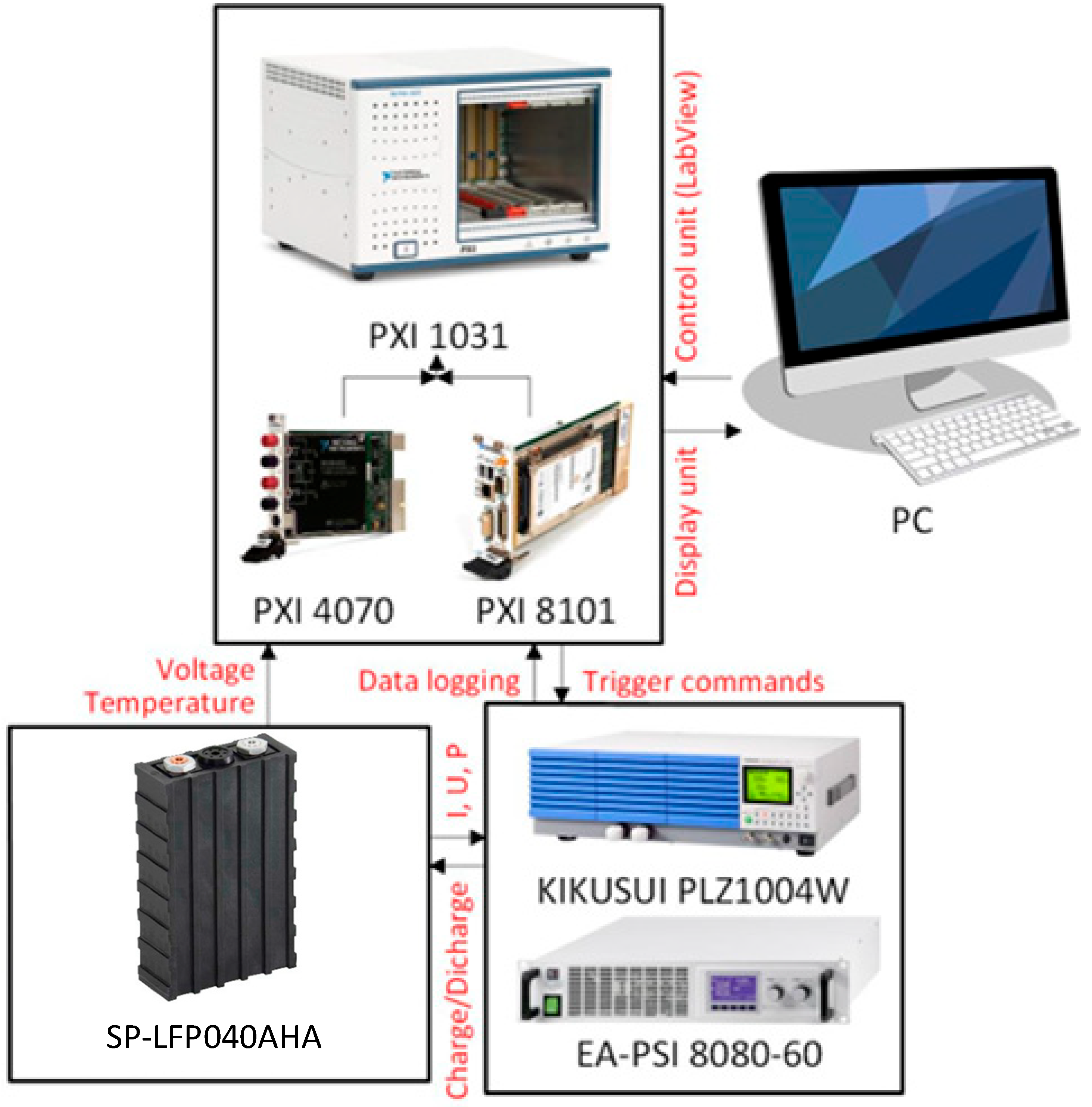
The two components of this system are a programmable source and a programmable load. Figure 2 shows the battery’s electrical identification system scheme. The LabVIEW (fy National Instruments) environment was used to construct the algorithm for these devices, which includes adjusting the voltage, current, and power parameters for charging and discharging. The cells’ temperature is simultaneously tracked, and if it rises too high, it is turned off. Two cards, PXI 4070 and PXI 8101, are connected to PXI 1031, which solves the control. A highly accurate multimeter is the PXI 4070 measuring card. The voltage on the cell and the voltage changes on the thermistor, a thermal sensor, are both monitored by this card. The PC and the load/source are connected via the PXI 8101 control card. This card has a serial connection with a programmable source and load, USB ports for a mouse and keyboard, and an HDMI port for attaching a screen. This serial communication is used to control these programmable devices. The cells are immediately connected to these gadgets, which are attached to a lockable cabinet. Using the observed current, the program can determine the battery’s capacity directly. This system has been modified to record measured values even when the battery is being charged, discharged, and unloaded. When charging or discharging, the algorithm has the ability to pause. When deciding on the EEC parameters, these pauses are crucial. These pauses allow us to measure the electrochemical cell’s regenerated voltage, which we can then use to calculate the open-circuit voltage (OCV).

The three primary components of the measurement infrastructure are depicted in Figure 2. The control section comes first. The PXI 8101 control card and the PXI 4070 measurement card are part of the PXI 1031 control and measurement unit. An algorithm operates in the LabVIEW environment on a PC that is attached to the PXI 8101 control card. In addition to storing the measured quantities, this method regulates the source and load. The active execution unit is the second component. It has the PLZ1004W programmable load and the EA-PSI 8080-60 programmable source. These gadgets are in charge of giving and taking energy from the cells. The load KIKUSUI PLZ1004W is programmable. This load can run up to 1 kW of power, 150 V of maximum voltage, and 200 A of maximum current. It operates at the cell level according to these criteria. One programmable power source is the EA-PSI 8080-60. With a maximum voltage of 80 V and a maximum current of 60 A, this source can run up to 1.5 kW. The terminals are connected to the source/load in a closed chamber, which is the final component of the measuring infrastructure. These terminals are contacts where the electrochemical cell or battery is directly powered. Battery racks, a thermistor, a camera, and a mechanical disconnector are all located in this chamber. The chamber is designed to test batteries or cells under extreme circumstances, such as overcharging, deep discharge, or short circuit. Figure 3 depicts the actual configuration of the measuring infrastructure.

4. Identification of Equivalent Electrical Replacement Scheme

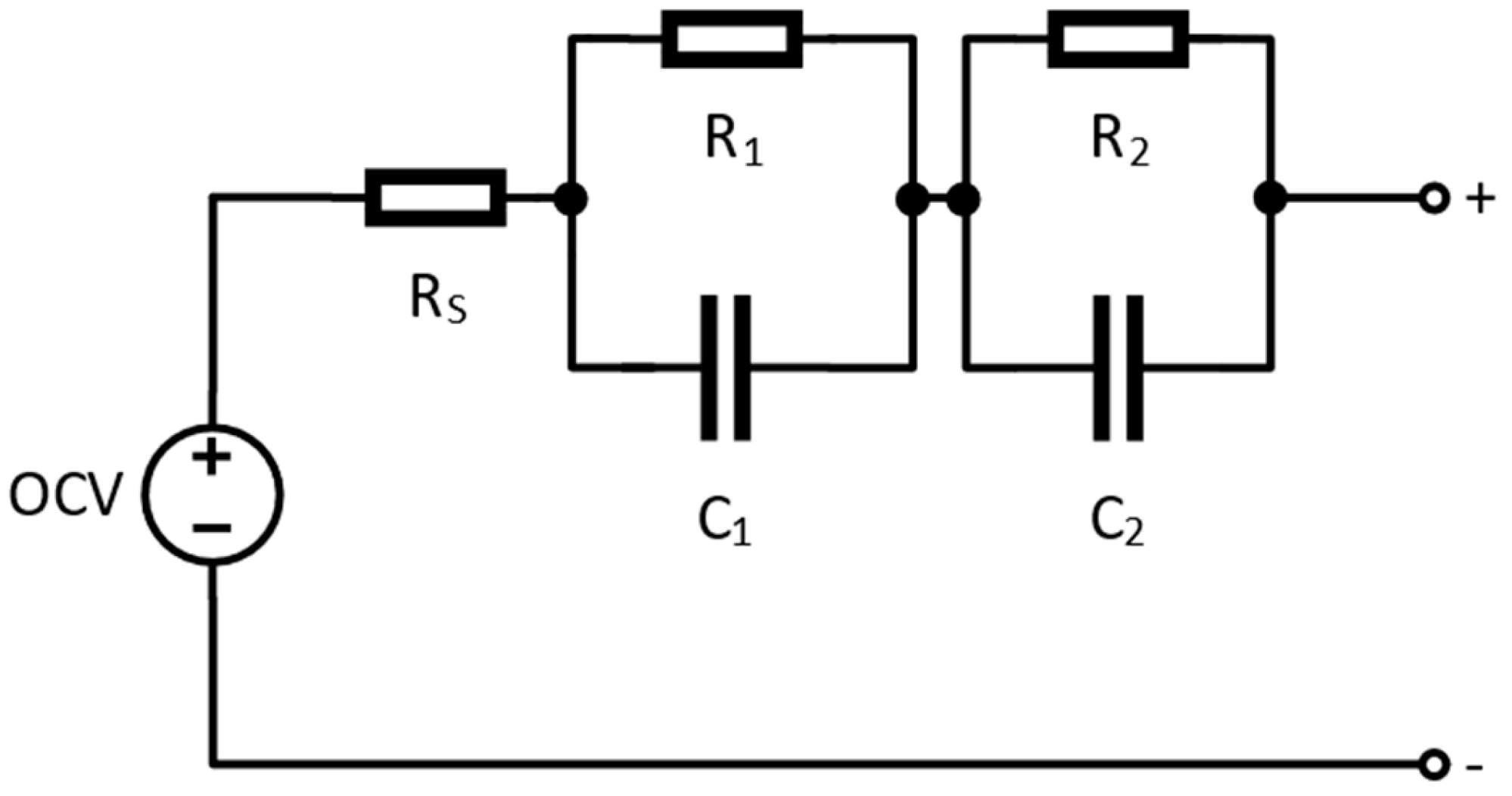
Figure 4 displays the corresponding circuit’s parameters. This is an illustration of the comparable c EEC, which is composed of several elements responsible for the physicochemical mechanism related to the degradation.

The resistance, R_s, results from both the ionic resistance within the electrolyte and the electronic resistance in the current collectors. Known as ohmic resistance, Rs represents the lowest real part of the impedance, as depicted in Figure 4. As frequency decreases, the Nyquist diagram displays only one semicircle, even though two would typically be expected [24]. This occurs because the individual contributions from each electrode cannot be distinctly separated. If the first semicircle were visible, it would correspond to the SEI layer and charge transfer processes occurring at both electrodes. Prior research suggests that lithiated transition-metal oxides (TMOs) form solid films due to complex surface interactions in alkyl carbonate electrolytes containing LiPF6 salts [25].

An equivalent electrical sub-circuit is employed to model this portion of the impedance spectrum, consisting of a resistance, R₁, in parallel with a non-ideal capacitor. This capacitor is represented by a constant phase element (CPE) with an exponent ranging from 0.8 to 1, denoted as C₁. At lower frequencies, key observed phenomena include solid-state diffusion and the capacitive effects associated with Li+ storage within the anode. However, because linking this section of the Nyquist spectrum to a Warburg-like pattern—typically characterized by a 45-degree slope in the diffusion tail—is challenging, the proposed equivalent electrical circuit (EEC) incorporates an additional resistance, R₂, in parallel with a capacitor, C₂.

R₂ is generally associated with the rate-limiting processes occurring within the electrode particles, independent of the specific microscopic mechanism involved, whether it be ion diffusion or electrochemical reactions. C₂, on the other hand, corresponds to the chemical capacitance.

The observed transport limitations may stem from the solid-state diffusion of lithium ions within the host material or from resistance-related barriers that impede lithium-ion alloying and conversion reactions within oxide-based matrices.

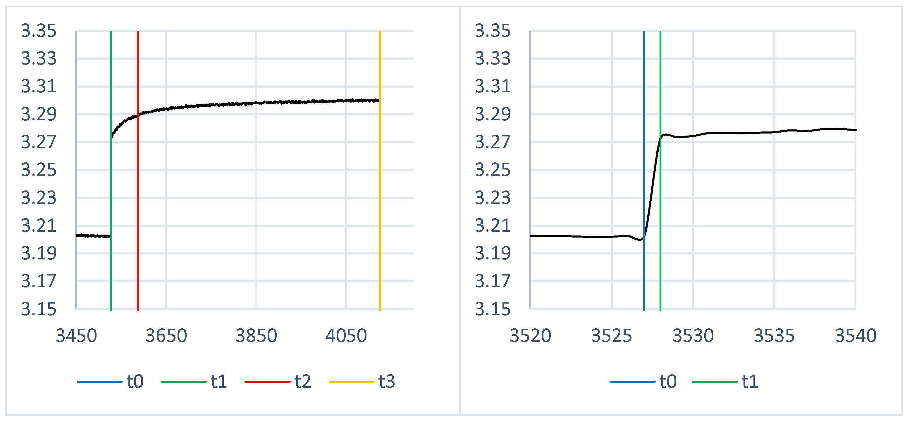
Five values make up the measured data, and they are recorded once every second. The cell voltage, temperature, and current passing through the cell are the measured parameters; the current power is computed using these data. The final value is determined by the algorithm. This represents the capacity that is currently charged or discharged. Every second, these five values are updated and recorded. These values serve as the foundation for all characteristics. It is essential to precisely document the electrochemical cell’s voltage recovery process when taking measurements with pauses. The regeneration time and the voltage differential before and after regeneration at specific intervals are then calculated by analyzing these pauses. The time constants required to determine the parameters of the analogous circuit are displayed in Figure 5, where t0 is the time before the battery discharge, t1 is the time in seconds following the termination of the load, t2 is the regeneration time 60 s following the termination of the load, and t3 is the time after 600 s [24]. The cell will be loaded in one second at this point. The internal resistance of the cell is determined by the voltage differential between t0 and t1. The voltage V0 (1) represents this. This is represented by the parameter R_S in Formula (4) for the EEC. The fast and slow time constants are represented by the voltage difference between t1 and t2 and the voltage difference between t2 and t3. The voltages V1 (2) (fast) and V2 (3) (slow) stand for this. In Formulas (5) and (7), the parameters of the equivalent circuit C₁ and R₁ stand in for the fast time constant. In Formulas (6) and (8), the quantities C₂ and R₂ stand in for the slow time constant. There were always pauses after 5% of the specified cell’s SoC. Depending on the change in SoC, it is feasible to ascertain how the parameters of the corresponding electrical circuit alter.

$$V_0=V_{t1}-V_{t0}$$

(1)

$$V_1=V_{t2}-V_{t1}$$

(2)

$$V_2=V_{t3}-V_{t2}$$

(3)

$$R_S={\displaystyle \frac{V_0}{I}}$$

(4)

$$R_1={\displaystyle \frac{V_1}{I}}$$

(5)

$$R_2={\displaystyle \frac{V_2}{I}}$$

(6)

$$C_1={\displaystyle \frac{t_2-t_1}{R_1}}$$

(7)

$$C_2={\displaystyle \frac{t_3-t_2}{R_2}}$$

(8)

5. Results

The charging and discharging of the cell is referred to as cell cycling. A single cycle represents a single cell charge and discharge. Only one type of cell was used for testing because cycling cells with larger capacities takes a lot of time. The SP-LFP040AHA cell was specifically cycled. A programmable load and a programmable power source were used to cycle, specifically, the EA-PSI 8080-60 power supply and the KIKUSUI PLZ1004W programmable load. Setting the maximum charging voltage to 3.65 V allowed for cycling. The discharge was stopped when the minimum cell voltage for discharging was set to 2.5 V. 60 A was the same current used for both charging and discharging. The process for evaluating the EEC parameters was applied to the cell prior to cycling. The cell was cycled 25 times after these parameters were established. The process for evaluating the parameters of the new electrical circuit was repeated after 25 cycles. The cell was then cycled 25 times more. The discharging process was realized with the constant current discharge (60 A), while the charging process was performed with the CC/CV profile (Figure 6).

The process for evaluating the new EEC parameters was then used once more. Until the SP-LFP040AHA cell was cycled 100 times, this was done every 25 cycles. The characteristics displayed below are the outcome of these measurements of the EEC parameters. These characteristics are 3D area graphs, with the cell’s energy content (SoC) on the x-axis, the value of the specified parameter on the y-axis, and the cell’s cycle count on the z-axis. This makes it simple to see how the internal parameters of the replacement electrical circuit change as a result of cycling.

Each 3D graph’s mathematical form is also shown below. Higher-order polynomial waveforms are displayed in their mathematical form. From the perspective of the simulation model, this mathematical representation is significant. Battery cell simulation models can be constructed from this data for every cycling value. Neural networks can also be input these mathematical representations. A mathematical estimate of how the parameters will change at higher cycling can be made using the neural network’s ability to process this data.

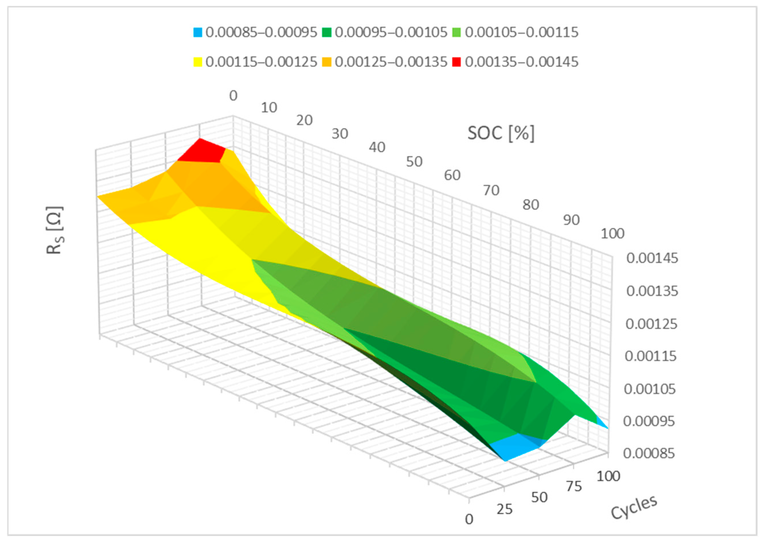
5.1. Parameter R_S

Figure 7 below illustrates the change in the R_S parameter’s dependency on cell energy as a function of the SP-LFP040AHA cell’s cycle count. It is evident that 100 cycles do not significantly affect the R_S parameter when it is changed. One could argue that the R_S parameter stayed essentially constant.

The waveforms from Figure 7 are mathematically represented by polynomials in Figure 8 below. The internal resistance of the R_S parameter increases slightly between 0 and 10% SoC, as seen in the picture, which might be associated with the formation of the passive film on the electrodes. A neural network can be used to forecast how the R_S parameter will evolve with additional cycling based on this 3D graph.

5.2. Parameter R₁

Figure 9 shows the cycling-induced change in parameter R₁. This graph illustrates how parameter R₁ evolved between 0% SoC and 10% SoC. It is obvious from this that the sector parameter R₁ is greater than it was prior to cycling. Here, it is possible to predict how more cycling will affect the value of parameter R₁. It is assumed that this parameter will change the most between 0% and 20% SoC.

The R₁ parameter can be represented mathematically as a polynomial, much like the R_S parameter in Figure 10. As illustrated in Figure 9, it is also evident in this case how cycling causes the resistance of the R₁ parameter to increase. The range between 0 and 10% SoC is where this resistance increase is most noticeable. It is reasonable to expect that when implementing a neural network, this parameter will primarily vary within the specified interval of 0–10% SoC as a result of additional cycling.

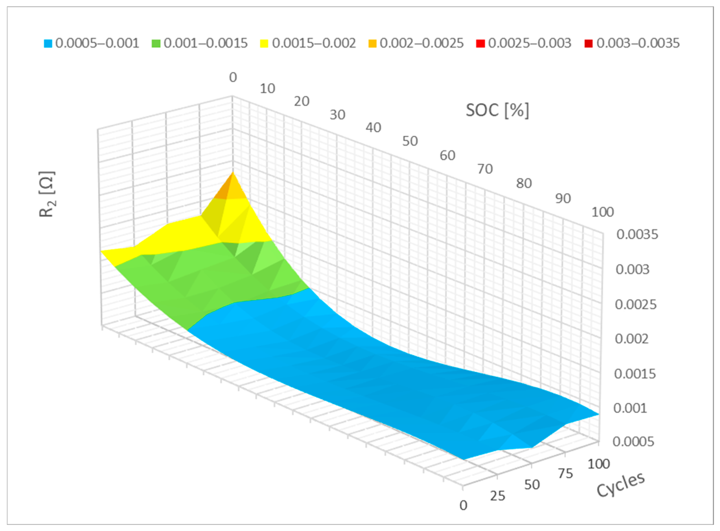
5.3. Parameter R₂

For parameter R₂, the difference is more apparent. It is evident from Figure 11 that the resistance of parameter R₂ increased between 0% and 20% SoC. It is possible to make assumptions about how it might change based on the cycling effect results. The resistance of parameter R₂ would rise more quickly in the range of 0% to 20% SoC with additional cycling. Changes in R₁ and R₂ can be associated with a change in the kinetics of electrochemical reactions.

The path of the mathematical representation of the measured data from Figure 11 can be observed in Figure 12, just like with the prior parameters. Specifically, it is parameter R₂ in this particular case. It is easy to see how parameter R₂ differs in this 3D graph. It is evident when cycling that the 0–10% SoC interval is crucial, similar to how it is for parameter R₁. Here, it can be presumed that the largest change will occur with additional cycles.

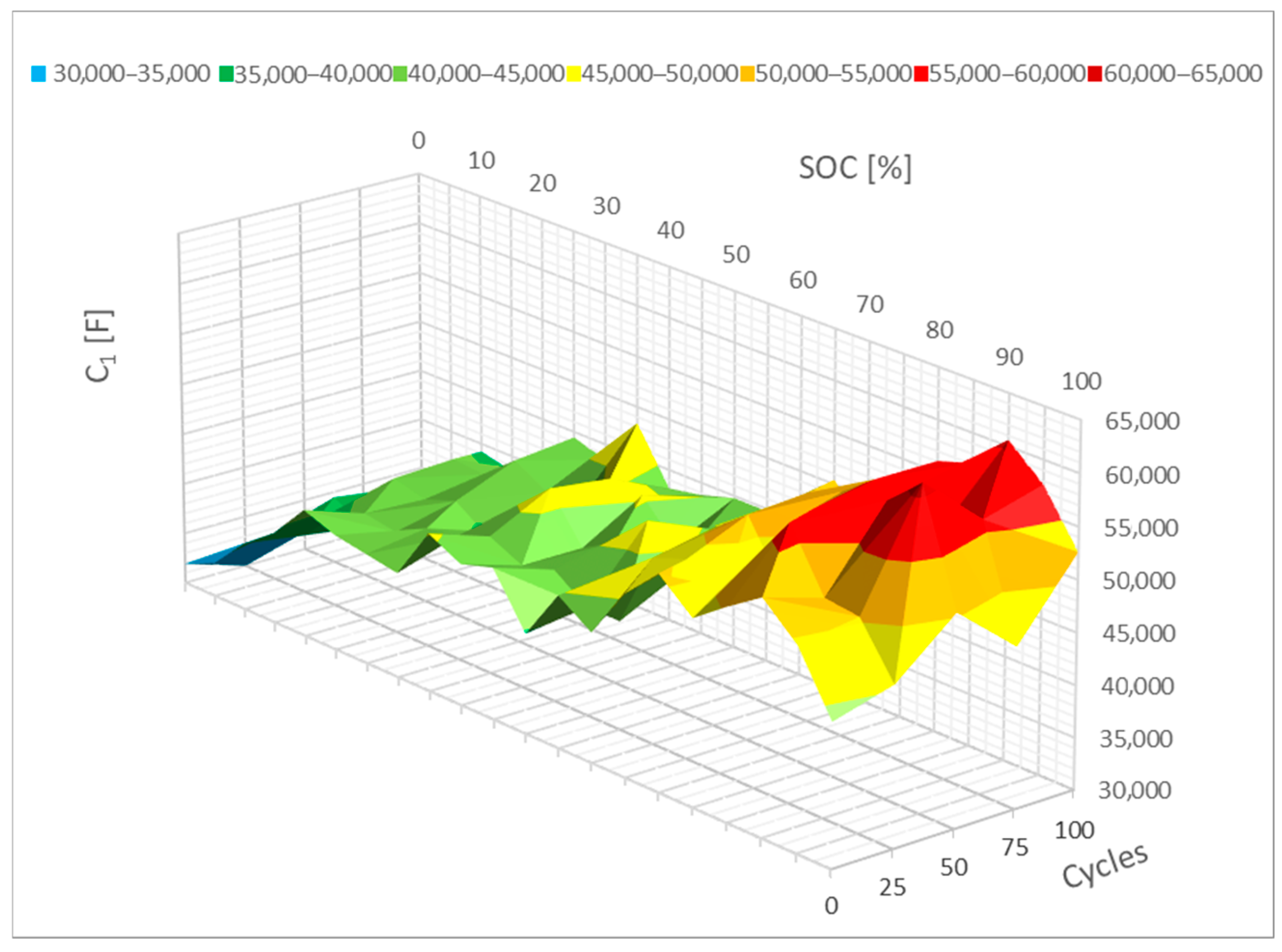
5.4. Parameter C₁

Figure 13 shows a lesser change in the value of the C₁ parameters. The cycle barely altered this parameter. It is also feasible to think that this value will primarily change between 0% and 20% SoC. In this case, it may be said that this parameter will drop as the resistance rises.

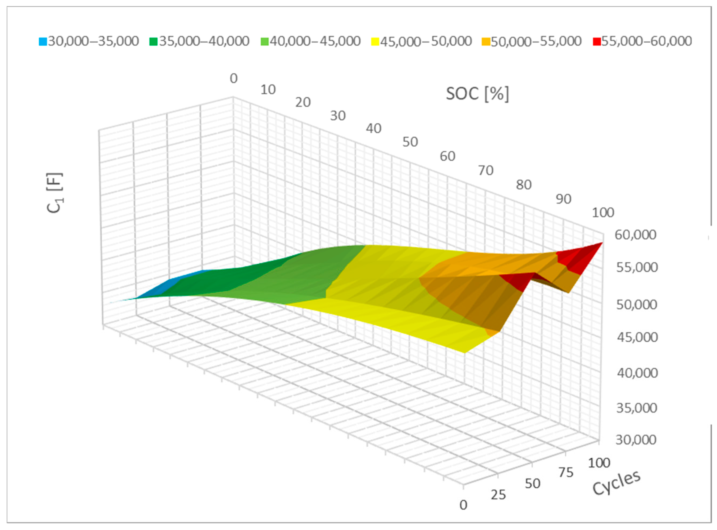
Similar to the R parameters, the C₁ parameter can also be represented mathematically, as in Figure 14, which shows how the C₁ parameter changed. In this case, a drop in the 0–20% SoC interval can be seen. It is also feasible to see a change in the interval between 80 and 100% SoC with this C₁ parameter; in this case, there is a minor increase. Therefore, it is reasonable to think that these changes may intensify if the cell cycles further.

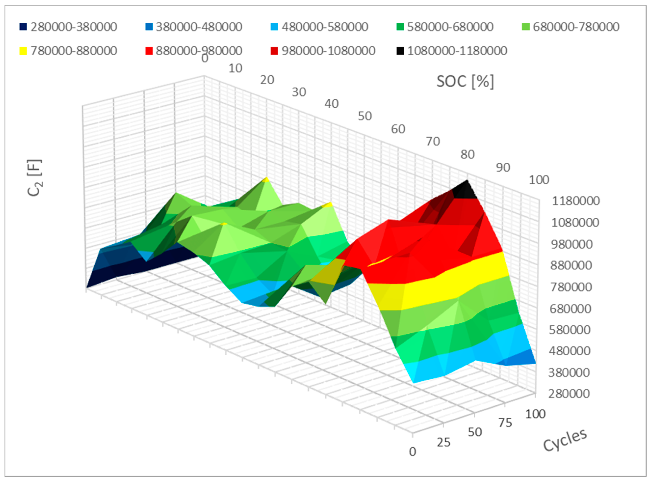
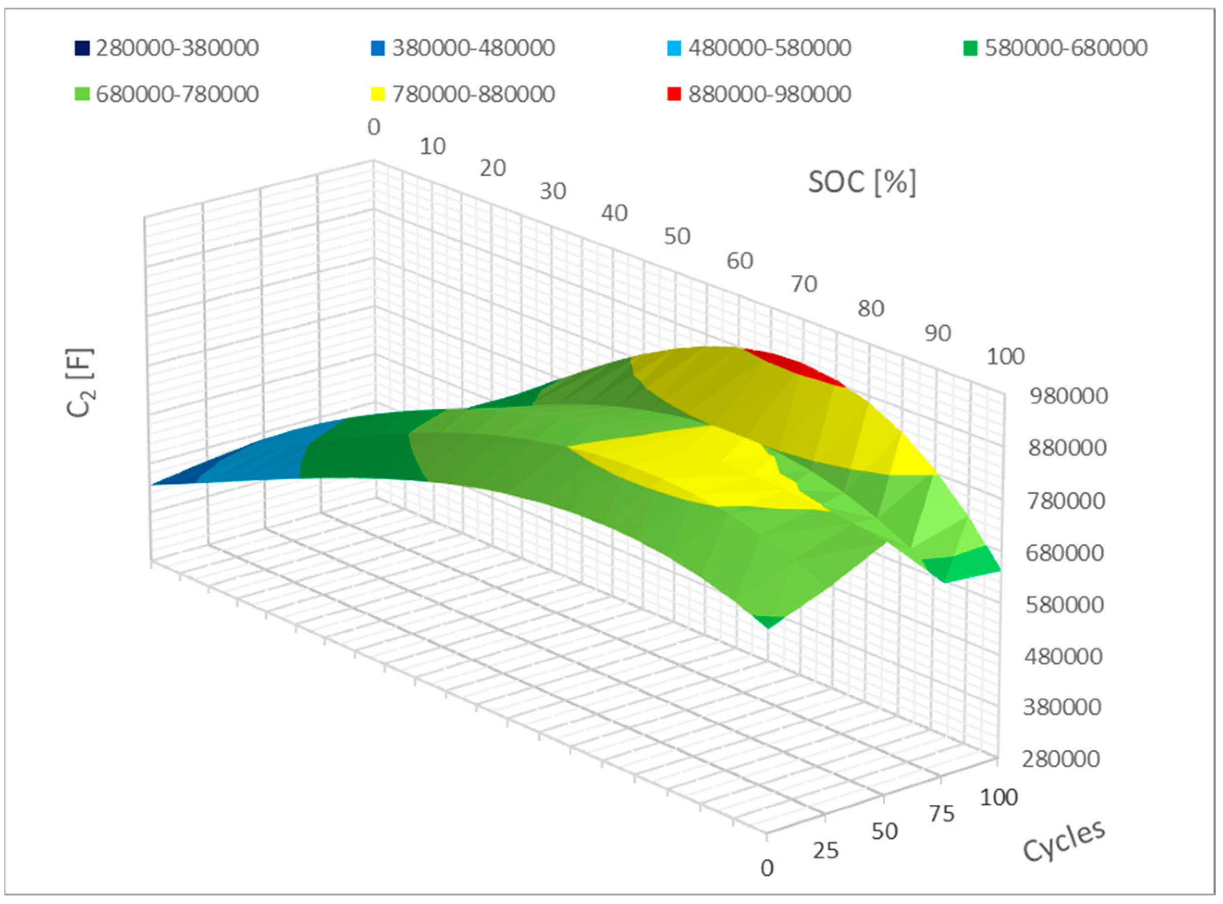
5.5. Parameter C₂

Figure 15 shows how parameter C₂ has changed. This alteration closely resembles parameter C₁’s. The range of 0% to 20% SoC will also see the most change for this C₂ metric. As internal opposition rises, this capacity will fall. Cycling may also result in a small increase in capacitance at 80% SoC.

Figure 16 shows the last parameter, C₂, in mathematical form, a situation quite close to that of parameter C₁. The capacity dropped during the 0–10% SoC interval, which likewise shows a change. A modest increase is observed once more in the 80–100% period. Another way to put it is that these changes will become more profound as the cell cycles more.

6. Discussion of the Mathematical Model of Aging Using Measured Data and Neural Networks

In order to create a mathematical model of cell aging and potential prediction of the SOH (state of health) parameter from the measured data, machine-learning methods were used. Among the machine-learning algorithms, the method of artificial neural networks was considered. The main reasons were the universality of the mathematical model of networks, the sophistication of optimization algorithms, and very good experience with the results of networks applied in various fields of technology and engineering.

The data consisted of the calculated parameters of the battery equivalent electrical circuit (model): RS, OCV, C1, R1, C2, and R2. The dimension of the input data within the mathematical model was 6. The parameters of the EEC in Figure 3 were represented by polynomials of higher orders (3 and 6), the waveform of which interpolated the experimentally measured waveform depending on the amount of energy in the cell (SoC). Within the methodology, the SoC parameter changed with a step of 1% and represented an independent variable for which polynomial values were determined. The parameters of the EEC were measured in a time period after 25 charge/discharge cycles. From the point of view of creating a dataset for the needs of machine learning, these were dependent variables, the values of which are a non-linear function dependent on the mentioned six parameters from Figure 10.

From the point of view of numerical mathematics, finding the internal parameters of a neural network represents the optimization task of minimizing the sum of squared errors between the target values and the model-predicted values. Levenberg–Marquardt (LMA) was chosen as the optimization algorithm. This optimization method is the default deterministic optimization method in the Matlab Neural Network Toolbox software (matlab 2024b) module. It generally provides fast convergence to a local/global minimum. In contrast to the Gauss–Newton method, which requires the calculation of the Hessian (the square matrix of the partial derivatives of the 2nd order of the error function according to the network parameters sought), the calculation is much faster. The Hessian is only approximated, while the memory and computing requirements are an order of magnitude lower.

Selection of Neural Network

The choice of the specific architecture of the artificial neural network was influenced by the range of input data, especially the number of input (six) and output parameters (one). The number of parallel instances (batches) of the six-dimensional input vector also had an effect on the resulting network architecture. The number of doses was about 500 and resulted from the step size of the state of charge (SoC) parameter, which varied in the interval (0–100%, step 1%) and the number of cycles within the experiment of determining the parameters of the replacement battery model. Given six input parameters, the number of input neurons was six with a sigmoidal activation function.

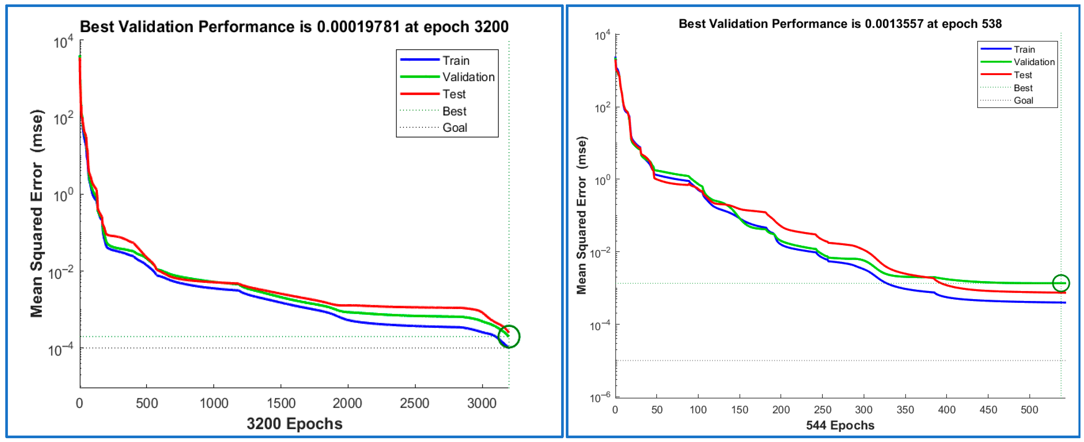
A forward neural network with two hidden layers was chosen, as the network with one hidden layer did not achieve sufficient performance in the decrease of the primary evaluation criterion of the mean value of the sum of squares of errors (mean square error). Figure 17 shows insufficient decay of the error function. Therefore, a network with two hidden layers and the number of neurons 6–4–1 was chosen. One output parameter requires one output neuron with a linear activation function. The proposed architecture is used by default in regression tasks and, if there are more neurons at the output, also in classification tasks. The improvements in the results can be observed in Figure 18.

In the figures, we can observe the consistency of the decrease of the error function on all three sets, which points to the good generalization properties of the model. The left part represents the application of machine learning in charging a lithium cell according to the manufacturer’s recommendations. The right part represents the same neural network, but applied to the parameters of a lithium cell that was intentionally overcharged and undercharged. In both cases, we can observe a significant decrease in the root mean square error in the range of more than six orders of magnitude.

Based on the presented introduction to the use of neural networks, future works are expected to follow the estimation methodology of the state of the health of the battery based on the measured data of the EEC components.

7. Conclusions

The parameters of the equivalent electrical circuit (EEC) undergo noticeable and progressive changes as the cell is cycled over time. Experimental findings from a detailed area graph analysis reveal that the interval between 0% and 10% state of charge (SoC) experiences the most substantial impact when cycling reaches up to 100 cycles. This key observation indicates that the early stages of charge depletion or replenishment play a crucial role in determining long-term performance degradation. By closely examining these graphs, the cycling-induced variations in EEC parameters become evident, providing valuable insight into the cell’s internal electrochemical behavior.

One particularly significant finding is the measurable increase in internal resistance, specifically in the parameter R_S. Across the entire SoC range from 0% to 100%, R_S demonstrates a consistent upward trend when compared to conventional cycling conditions. This resistance buildup suggests that the cumulative effects of cycling contribute to an overall decline in efficiency, reinforcing the notion that repeated charge–discharge cycles negatively impact the cell’s structural integrity. Notably, these effects persist even when cycling conditions adhere to the manufacturer’s recommended operational criteria, implying that standard cycling practices may still lead to progressive degradation over time.

In addition to resistance changes, this study delves into the evolving mathematical representations of the measured waveforms. These representations are critical for understanding how the underlying electrical characteristics of the cell shift as cycling progresses. In particular, when considering the simulation model of the SP-LFP040AHA cell, these refined mathematical formulations prove invaluable. By integrating these representations into simulation frameworks, researchers can construct highly detailed models capable of accurately depicting cell behavior under various cycling conditions. Such models not only allow for comprehensive analyses of SoC variations but also provide a crucial link to tracking the long-term state of health (SOH) degradation.

Beyond traditional analytical methods, this dataset presents promising opportunities for advanced computational applications. For instance, neural networks can leverage this information as input, enabling predictive modeling of parameter evolution over extended cycling periods. The 3D graphical outputs serve as a powerful tool for assessing trends in key variables, allowing researchers to ascertain the rate and extent of parameter shifts with remarkable precision. Through these insights, engineers can develop highly refined projections of how EEC parameters transform as a function of cycling intensity, providing critical knowledge for optimizing battery performance and durability.

This comprehensive investigation underscores the necessity of integrating experimental findings into advanced modeling approaches. By bridging empirical observations with computational techniques, researchers can formulate more effective strategies for enhancing battery reliability, extending lifespan, and improving predictive maintenance protocols. These findings contribute to the broader field of energy storage research, offering key insights into how cycling affects cell behavior and paving the way for innovative solutions in next-generation battery technology.