Abstract
In this study, the particle swarm optimization (PSO) and back propagation neural network (BPNN) surrogate model in combination with a multi-objective genetic algorithm are developed for the design optimization of a bionic liquid cooling plate with a spider-web channel structure. The single-factor sensitivity analysis is first conducted based on the numerical simulation approach, identifying three key factors as design variables for optimizing design objectives such as maximum temperature (Tmax), maximum temperature difference (ΔTmax), and pressure drop (ΔP). Subsequently, the PSO algorithm is used to optimize the parameters of the BPNN structure, thereby constructing the PSO-BPNN surrogate model. Next, the non-dominated sorting genetic algorithm II (NSGA-II) is employed to obtain the Pareto optimal set, and the TOPSIS with the entropy weight method is used to determine the optimal solution, eliminating subjective preferences in decision-making. The results show that the PSO-BPNN model outperforms the traditional BPNN in prediction accuracy for all three objectives. Compared to the initial structure, the Tmax and ΔTmax are reduced by 1.09 °C and 0.41 °C in the optimized structure, respectively, with an increase in ΔP by 21.24 Pa.
1. Introduction
Due to increasingly severe energy shortages and environmental degradation, countries around the world have begun to develop more energy-efficient and environmentally friendly electric vehicles, which are gradually replacing traditional fuel vehicles and becoming the main trend of future automotive development [1,2]. Lithium-ion batteries are the core power source for electric vehicles and have become widely used in the electric vehicle sector because of their high energy density, low self-discharge rate and long cycle life [3,4]. However, the operating temperature of lithium-ion batteries significantly affects their performance and lifespan. The ideal operating temperature range is 25 °C to 40 °C, and the ΔTmax should be controlled within 5 °C [5]. If the temperature exceeds the maximum safety threshold of lithium-ion batteries, it may result in thermal runaway, potentially triggering serious safety accidents such as fires and explosions [6,7]. Therefore, establishing an efficient battery thermal management system (BTMS) is extremely important for ensuring the safe and stable operation of the batteries.
Battery thermal management approaches primarily consist of air cooling [8,9], liquid cooling [10,11], phase change material (PCM) cooling [12,13], and heat pipe cooling [14,15]. In the past, air cooling was widely applied due to its advantages, such as simple structure and low maintenance cost [16]. However, as the energy density of batteries rises, air cooling is unable to satisfy the heat dissipation requirements [17]. Although PCM can effectively absorb the heat generated by batteries, it has not been applied due to its poor thermal conductivity [18]. Heat pipes possess good thermal conductivity but generally need to be combined with other cooling approaches, which increases system complexity [19], thus limiting their application in BTMS. In comparison, liquid cooling remains the mainstream form of thermal management for batteries because of its outstanding heat dissipation capability [20].
Liquid cooling can be categorized into two types: direct contact cooling and indirect contact cooling [21]. In direct contact cooling, the coolant makes contact with the battery for heat exchange, providing better temperature uniformity for the battery, which, however, requires high-stability dielectric coolant and a well-sealed cooling system [22]. In comparison to direct contact cooling, indirect contact cooling employs the liquid cooling plates to establish a connection with the batteries, with thermal interface materials in between them to dissipate heat. The key design principle for the liquid cooling plate is to create a reasonable flow channel to ensure that the coolant is evenly distributed in the channels. Li et al. [23] studied the impact of two layouts of liquid cooling plates with a single channel, multiple small channels, and an S-shaped channel on the thermal management of the battery module. The results indicated that placing liquid cooling plates with multiple small channels on both sides of the battery module achieved optimal cooling performance. Sheng et al. [24] devised a liquid cooling plate with double serpentine channels, finding that the arrangement of the inlet and outlet significantly affected the temperature difference. Huang et al. [25] designed a liquid cooling plate with streamlined channels, and the results showed that it can significantly reduce ΔTmax and ΔP.
Besides the conventional liquid cooling plates mentioned above, researchers have shown interest in the design of liquid cooling plates inspired by bionic structures. Wang et al. [26] designed a liquid cooling plate with a butterfly-shaped flow channel and compared its cooling performance with straight, serpentine, and leaf-shaped liquid cooling plates. The results showed that the butterfly-shaped liquid cooling plate demonstrated superior overall performance. Subsequently, further optimization of its structural parameters resulted in an optimal configuration, reducing the Tmax to 32.72 °C and ΔP to 25.7 Pa. Liu et al. [27] proposed a bionic leaf-vein channel liquid cooling plate and studied the impact of various structural factors. It was found that the channel width and inlet velocity significantly affected the cooling performance. Fan et al. [28] designed four types of liquid cooling plates with bionic fishbone channels. Compared to the Z-shaped liquid cooling plate, the bionic fishbone channel liquid cooling plate with a single inlet and dual outlets demonstrated better cooling performance.
In most cases, the above methods for optimizing battery thermal management parameters primarily rely on numerical simulations and tedious case experiments. The diverse and complex combinations of different parameters result in the significant consumption of time and computational resources during the analysis and optimization processes. As diverse surrogate models and artificial intelligence algorithms evolve, large amounts of data can be processed quickly, improving work efficiency without human intervention. As such, many researchers have optimized BTMS using surrogate models and optimization algorithms. Due to the nonlinear characteristics of complex BTMS, the BPNN is used as a surrogate model for multi-objective optimization because of its advantages in handling complex nonlinear mapping relationships and strong self-learning ability. Li et al. [29] used an artificial neural network to establish the relationship between battery spacing, ambient pressure, and both the Tmax and ΔTmax and then improved the temperature uniformity of the battery module through optimized design. Chen et al. [30] showed that a deep learning neural network model provided more precise output predictions for the cooling performance of carbon/epoxy resin with a microchannel compared to the response surface model. Although progress has been made in performance prediction, the traditional BPNN has certain limitations as a surrogate model. The learning rate and the number of hidden nodes, which are critical hyperparameters affecting model training, are generally set based on personal experience and often require multiple human trials to optimize. Additionally, the initial weights and thresholds of the BPNN are generally initialized randomly, which would lead to the network getting stuck in local optima during training, thereby affecting the prediction performance of the model.
In response to the above issues, this paper introduces the PSO-BPNN surrogate model in combination with multi-objective genetic algorithm for the design optimization of a bionic liquid cooling plate constructed with a spider-web channel structure. The PSO algorithm can automatically optimize the number of hidden nodes, learning rate, initial weights, and thresholds without human intervention. This approach significantly enhances the prediction accuracy of the BPNN. Based on this, a novel spider-web liquid cooling plate is proposed, with the Tmax, ΔTmax, and ΔP selected as optimization objectives. The optimal Latin hypercube sampling (OLHS) method is employed for sampling, and a corresponding dataset of samples is constructed through computational fluid dynamics (CFD) simulations. Based on these data, the PSO-BPNN surrogate model is established. Subsequently, the NSGA-II algorithm is adopted to perform multi-objective optimization on the spider-web cooling plate. The entropy weight method is used to determine the weight of each objective, and the TOPSIS method is applied to rank the optimal solutions, thereby obtaining the optimal structural parameters for the cooling plate.
2. Model and Validation
2.1. Model Description
A bionic liquid cooling plate with a spider-web channel is designed for battery thermal management. The prismatic lithium-ion battery used in this paper is of the model CATL2795148-51Ah. Its cathode material is LiNi0.8Co0.1Mn0.1O2, the anode material is graphite, and the electrolyte is LiPF6. The detailed characteristic parameters are listed in Table 1. The geometric model of the battery liquid cooling system is shown in Figure 1, which consists of five batteries and six liquid cooling plates arranged alternately. It is noted that the liquid cooling plates are positioned on the large sides of the batteries. When prismatic lithium-ion batteries are grouped, the large sides with the highest temperature come into contact, making it difficult for the heat generated by the batteries to dissipate in time, leading to heat accumulation. As such, a side-contact cooling method is adopted to enhance the heat dissipation of the batteries. To save computational resources, a representative cooling unit will be used as the subject of subsequent simulations, namely a liquid cooling plate in direct contact with two batteries. Considering that aluminum has good thermal conductivity and lightweight properties, it is selected as the material for the liquid cooling plate. Water flows through the channels in the liquid cooling plate, absorbing heat from the batteries. The physical parameters of the liquid cooling plate and coolant are presented in Table 2.

Table 1.
Parameters of prismatic lithium-ion battery.
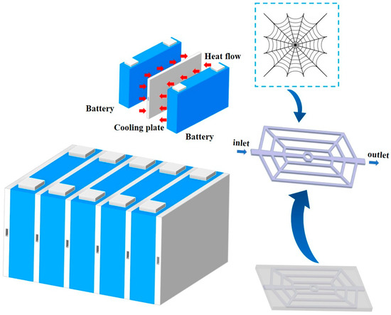
Figure 1.
Schematic of battery liquid cooling system.
Table 2.
Physical parameters of liquid cooling plate and coolant.
2.2. Governing Equations and Boundary Conditions
To improve the efficiency of numerical calculations, the following assumptions are made for the model.
(1) Radiative heat transfer between the battery and the surroundings is ignored.
(2) The coolant is incompressible with steady-state flow field.
(3) The physical properties of the coolant, liquid cooling plate, and battery are unaffected by temperature.
(4) The contact thermal resistance between the battery and the liquid cooling plate is ignored.
2.2.1. Battery Governing Equation
Assuming that the battery is composed of anisotropic and uniformly distributed materials, the three-dimensional energy equation for the battery in a Cartesian coordinate system is as follows [31]:
where ρbat, cbat, and Tbat are the density, specific heat capacity and temperature of the battery, respectively. λx, λy, and λz are the thermal conductivity of the battery along the x, y and z directions, respectively. q is the volumetric heat generation rate of the battery.
2.2.2. Convective Boundary Between Air and Battery
The convective boundary condition between the battery and the air is as follows [32]:
where hsur,bat is the convective heat transfer coefficient on the battery surface, and Ta is the ambient temperature.
2.2.3. Heat Transfer Boundary Between Battery and Liquid Cooling Plate
The heat transfer boundary condition and initial condition between the battery and the cooling plate are as follows [32]:
where λlcp is the thermal conductivity of the liquid cooling plate, and n is the normal direction.
2.2.4. Coolant Governing Equations and Boundary Condition
The coolant mass, energy and momentum conservation equations are as follows [33]:
Mass conservation:
Energy conservation:
Momentum conservation:
where ρf is the density of the coolant, is the velocity vector, cf is the specific heat capacity of the coolant, λf is the thermal conductivity of the coolant, Tf is the temperature of the coolant, μ is the dynamic viscosity of the coolant, ∇2 is the Laplacian operator, and Pf is the static pressure of the coolant.
The boundary condition between the liquid cooling plate and the coolant can be expressed as follows [32]:
For fluid flow, the Reynolds number can be calculated by Equation (11).
where D is the hydraulic diameter of inlet channel. After calculation, the Reynolds number at the maximum inlet velocity and maximum hydraulic diameter is 2181, which is less than 2300. As such, for the other cases where the Reynolds number is always below 2300, the standard laminar flow model is adopted for numerical calculations.
2.3. Verification of Grid Independence
The accuracy and speed of computations are affected by the number of grids in the model. To enhance the reliability of the simulation results, the grid independence test is performed. The polyhedral grid configuration is adopted for the grid division. The Tmax of the battery and ΔP are used as criteria for the grid independence test. The simulation results for various grid numbers are shown in Figure 2. It is indicated that with the number of grids increasing, the Tmax and ΔP tend to stabilize, and when the number of grids is more than 448,838, the Tmax and ΔP increase by 0.01% and 0.36%, respectively. Considering both computational accuracy and cost, the grid number at this point is ultimately selected for subsequent simulations.
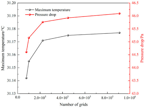
Figure 2.
Results of grid independence analysis.
2.4. Experiment of Heat Generation Rate
Based on the principle of the calibrated calorimetry method [34], the heat generation rate of a 51 Ah prismatic lithium-ion battery was tested. The experimental setup for the heat generation rate test was shown in Figure 3a. The testing system mainly included the battery, charge/discharge equipment (NEWARE CT-4008-5V60A-NFA, manufactured in China), thermostat (WBE 3SDG100L, manufactured in China), computer, and temperature data-acquisition instrument (HIOKI LR8410R, manufactured in Japan). Six thermocouples were distributed along the diagonal lines of the front and rear surfaces of the battery. The positive and negative terminals of the lithium-ion battery were connected to copper wire terminals using bolts and washers. The surface of the battery was covered with a 10 mm thick aerogel layer, which was secured with high-temperature tape to reduce heat dissipation during the experiment and establish an approximately adiabatic environment. The wrapped battery was placed in the thermostat, and all thermocouples were connected to a real-time data-acquisition instrument. The charge/discharge equipment was connected to the battery through copper wire terminals, and the computer controlled the discharging programs of the battery. Figure 3b showed the transient volumetric heat generation rate of the battery calculated using the calibrated calorimetry method under the 1C discharge rate.
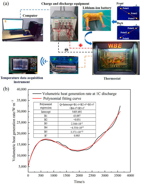
Figure 3.
(a) Schematic of the heat generation rate testing experimental system, (b) volumetric heat generation rate over time.
2.5. Verification of the Thermal Model
To validate the accuracy of the battery thermal model, a numerical transient simulation is conducted on the thermal behavior of the battery under 1C discharge condition. Considering that the heat generation rate of the battery during 1C discharge varies with time, the user-defined function (UDF) compiler in Fluent 2021R1 is employed to define the battery heat source. A simulation calculation is performed for the battery discharging at 1C in an ambient temperature of 25 °C, and the calculated average surface temperature of the battery is compared with the experimental temperature data from the 1C discharge of the battery, as shown in Figure 4. The maximum relative error between the simulated temperature and the experimental temperature does not exceed 3%. The results demonstrate good consistency, indicating that the battery thermal model possesses high reliability and is suitable for simulation analysis of battery cooling.
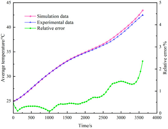
Figure 4.
Average temperature comparison between simulation and experiment.
3. Optimization Procedure
3.1. Establishment of the PSO-BP Surrogate Model
3.1.1. Design of Experiment
Before establishing the surrogate model, sample points must be obtained through experimental design. Based on the sensitivity analysis of the factors, as will be discussed in the later part of this paper, the channel width (X1), channel depth (X2) and inlet velocity (X3) are selected as the input variables for the experimental design, with the Tmax, ΔTmax, and ΔP as the output variables. The optimal Latin hypercube sampling (OLHS) method is employed for case sampling since it allows the sample points to be more uniformly distributed across the entire sampling space, unlike the Latin hypercube sampling (LHS) method [35]. A total of 95 sample points are selected using the OLHS method, and their distribution is plotted in Figure 5, which displays relatively uniform distribution within the design range. Subsequently, numerical simulations are conducted to calculate the output response values for each sample point.
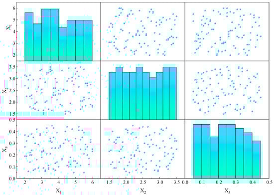
Figure 5.
Distribution of optimal Latin hypercube sample points.
3.1.2. BP Neural Network Model
BPNN is a feedforward neural network trained using the back propagation algorithm, suitable for solving complex nonlinear problems. As illustrated in Figure 6, the BPNN model comprises an input layer, a hidden layer, and an output layer. The input layer includes three nodes, which are the channel width (X1), the channel depth (X2), and the inlet velocity (X3). Similarly, the output layer includes three nodes, corresponding to the Tmax, ΔTmax, and ΔP. The number of hidden nodes is crucial for the prediction accuracy of the network. Therefore, the effect of the number of hidden nodes on prediction performance is taken into account. The number of hidden nodes, h, can be calculated by Equation (12). The output response values of the sample points obtained from numerical simulations are utilized to construct the dataset for the BPNN model, with 80% of the data allocated for training the surrogate model and 20% for testing the accuracy of the model.
where h, m, and n are the number of nodes in the hidden layer, input layer and output layer, respectively. a is an adjusting constant ranging from 1 and 10. In order to achieve higher prediction accuracy and avoid overfitting, the optimal number of hidden nodes is determined through the PSO algorithm.
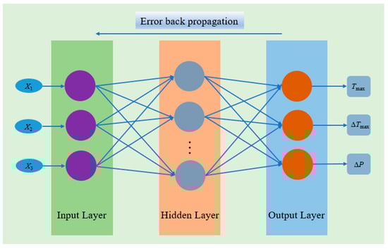
Figure 6.
Diagram of BPNN topology structure.
3.1.3. Particle Swarm Optimization Algorithm
The PSO algorithm is a heuristic intelligent optimization algorithm that simulates the foraging behavior of birds through iterative updating of particles to solve problems [36]. Each particle has its own unique position and velocity. The position of a particle stands for a potential solution, and its velocity determines the direction and magnitude of movement during the iteration process. The fitness function is used to evaluate the quality of each potential solution, and the entire population moves toward the optimal solution. Through continuous iteration of the velocity and position of particles, the optimal solution is obtained. The schematic diagram of the velocity and position updates during the iteration process is shown in Figure 7, and the corresponding update formulas are as follows:
where and are the velocity of the i-th particle in the j-th dimension at the t-th and (t + 1)-th iteration, respectively. and are the position of the i-th particle in the j-th dimension at the t-th and (t + 1)-th iteration, respectively. w is inertia weight, c1 and c2 are learning factors, and r1 and r2 are random values within the interval (0, 1). is the individual optimal solution of the i-th particle in the t-th iteration and is the global optimal solution in the t-th iteration.
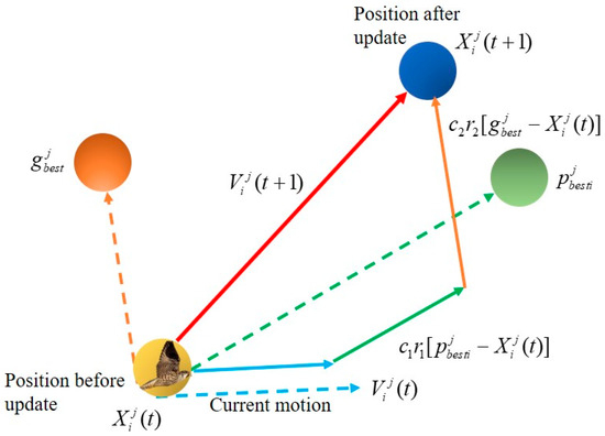
Figure 7.
Particle velocity and position update diagram.
3.1.4. BPNN Model Optimized with Particle Swarm Optimization
Based on the limitations of the traditional BPNN, this paper introduces the PSO algorithm to optimize the two critical hyperparameters of the BPNN, as well as the initial weights and thresholds of the nodes. Specifically, the PSO algorithm exerts its global search capability within the search domain by utilizing the prediction error of the BPNN as the fitness function of the PSO algorithm. This process continues until the algorithm identifies the optimal combination of the number of hidden nodes, learning rate, initial weights, and thresholds that satisfy the error precision requirements. These globally optimal solutions obtained after the algorithm terminates are assigned to the BPNN to achieve higher prediction accuracy. The specific algorithm flow is illustrated in Figure 8.
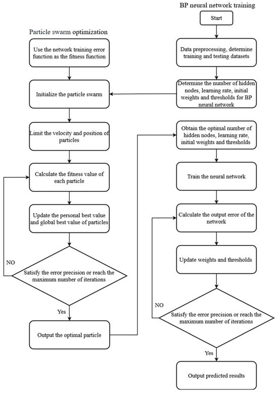
Figure 8.
Flow of the PSO-BPNN algorithm.
3.2. Mathematical Model of Multi-Objective Optimization
In the design of the spider-web liquid cooling plate, numerous variables interact with each other, and thus, a comprehensive assessment of the cooling performance is necessary. However, the combinations of different variables are complex and diverse, resulting in difficulty in the analysis and optimization processes, requiring substantial computational resources and time. In such circumstances, multi-objective optimization algorithms can be resorted to identify the optimal design scheme.
Based on the previously established PSO-BPNN surrogate model, the NSGA-II algorithm is employed to optimize the parameters of the spider-web liquid cooling plate. The channel width (X1), channel depth (X2) and inlet velocity (X3) are selected as the optimization variables, while the Tmax, ΔTmax, and ΔP are set as the optimization objectives. The general mathematical expressions are as follows:
3.3. TOPSIS with the Entropy Weight Method
In order to fully consider the differences in contribution among different objectives, it is particularly important to evaluate the three optimization objectives and allocate corresponding weights to them. The TOPSIS with the entropy weight method is employed to comprehensively evaluate and rank the Pareto optimal solutions.
3.3.1. Entropy Weight Method for Determining Weights
The entropy weight method is an objective weighting method which is used to assess the importance and dispersion of the objectives [37]. A higher entropy value indicates more concentrated information and a smaller weight, while a lower entropy value indicates more dispersed information and a larger weight. By calculating the entropy values, the weights of each objective can be determined, thereby influencing the comprehensive evaluation results. The calculation procedures of the method are as follows:
- (1)
- The initial decision matrix is as follows:
- (2)
- Data normalization is calculated by Equation (18).
- (3)
- The entropy value Sj is calculated by Equations (19) and (20).
- (4)
- The weight wj is calculated by Equations (21) and (22).
3.3.2. Decision-Making Using the TOPSIS Method
The TOPSIS method determines the relative priority of each Pareto solution by constructing a positive ideal solution and a negative ideal solution, which can objectively reflect the gaps between Pareto solutions and reduce the uncertainty caused by decision-makers’ preferences or differences in subjective judgments, thereby effectively addressing decision-making problems within the Pareto optimal solution set [38]. The calculation procedures of the method are as follows:
- (1)
- The weighted normalized matrix is as follows:
- (2)
- The positive ideal solution and the negative ideal solution are determined by Equations (24) and (25).
- (3)
- The distances of each Pareto solution to the positive ideal solution and the negative ideal solution are calculated by Equations (26) and (27).
- (4)
- The relative closeness of each Pareto solution fi is calculated by Equation (28).
4. Results and Analysis
4.1. Comparison of Cooling Performance of Different Cooling Plates
To verify the performance advantages of the spider-web liquid cooling plate, a comparison is made with straight and serpentine liquid cooling plates. The geometric shapes of the three flow channels are shown in Figure 9. The cooling performance of liquid cooling plates can be influenced by various parameters of the internal flow channel structure, including inlet size, channel depth, channel width, and the cross-sectional area of the flow channels. As such, to better compare the cooling performance of different liquid cooling plates, it is necessary to ensure that the dimensional parameters among different liquid cooling plates are as consistent as possible. The basic dimensions for the three flow channels are listed in Table 3. The three liquid cooling plates have a uniform thickness of 4 mm. Additionally, the cross-sectional areas and volumes of the flow channels are almost the same, with the weight of the liquid cooling plates differing by less than 0.5%.
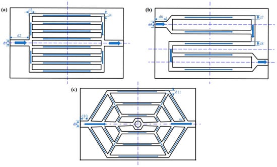
Figure 9.
Types of channel structures: (a) Straight channel, (b) Serpentine channel, (c) Spider-web channel.
Table 3.
Parameter settings of three channel structures.
The temperature contour plots of the batteries and pressure contour plots of three types of liquid cooling plates are shown in Figure 10. The corresponding data for the Tmax and ΔP are listed in Table 4. It is evident that the Tmax of the batteries is the highest in the straight flow channel, followed by the serpentine flow channel, and the lowest in the spider-web flow channel. As such, the cooling performance of the liquid cooling plate with the spider-web flow channel is better than the other two cases. In terms of ΔP, the advantage of the spider-web flow channel is more pronounced, with a significantly smaller ΔP compared to the other two flow channels. In contrast, the ΔP is highest for the serpentine flow channel structure, and the increased ΔP will result in higher power consumption of the pump. On the whole, the spider-web flow channel is superior to the other two flow channels in both cooling performance and power consumption. Hence, further optimization and research on the spider-web flow channel will be conducted in the following sections.
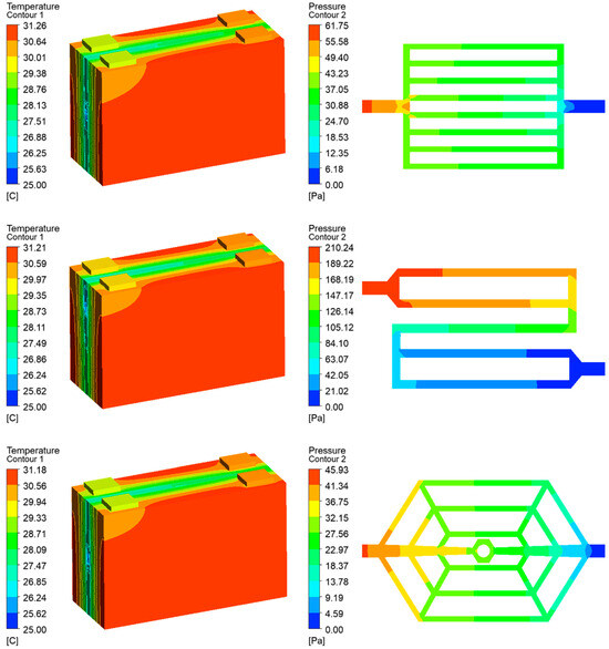
Figure 10.
Temperature contour plots of the batteries and pressure contour plots of three types of liquid cooling plates.
Table 4.
The data for the Tmax of the batteries and the ΔP.
4.2. Analysis of Different Influencing Factors
4.2.1. Influence of the Number of Branch Channels
The variation in performance is explored as the number of branch channels increases from 2 to 8, with an inlet velocity of 0.1 m·s−1, a channel width of 3 mm, a channel depth of 2 mm, and a channel angle of 60°. The variation curves of the Tmax, ΔTmax, and ΔP with the number of branch channels are shown in Figure 11. With the increase in the number of branch channels, the Tmax, ΔTmax, and ΔP all decrease. When the number of branch channels is 2, the Tmax is 31.49 °C, the ΔTmax is 4.74 °C, and the ΔP is 67.39 Pa. When the number of branch channels increases to 8, the Tmax decreases to 31.08 °C, the ΔTmax decreases to 4.67 °C, and the ΔP decreases to 42.38 Pa. The main reason is that with the increase in the number of branch channels, the contact area between the fluid domain and the solid domain within the liquid cooling plate increases, resulting in enhanced thermal convection at the interface. At the same time, the increased cooling channel length effectively extends the heat exchange time between the coolant and the wall, thereby reducing the Tmax. Furthermore, the increase in the number of branch channels reduces the coolant flow velocity in each channel, which leads to a reduction in ΔP. Based on the above analysis, the liquid cooling plate with eight branch channels demonstrates better cooling performance and lower ΔP. As such, a liquid cooling plate with an eight-branch channel structure is selected for further research.
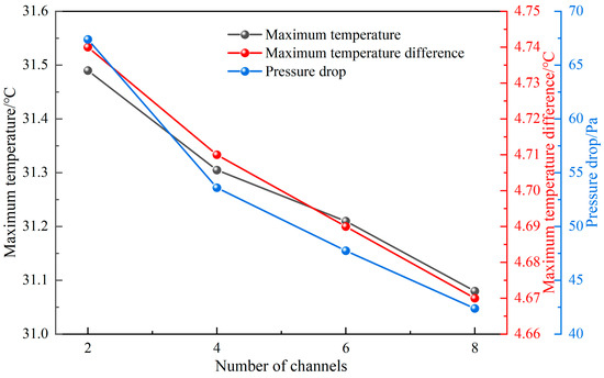
Figure 11.
Influence of the number of branch channels on Tmax, ΔTmax, and ΔP.
4.2.2. Influence of Different Inlet Velocity
The variation in performance is explored as inlet velocity increases from 0.05 m·s−1 to 0.45 m·s−1, with eight branch channels, a channel width of 3 mm, a channel depth of 2 mm, and a channel angle of 60°. The variation curves of the Tmax, ΔTmax, and ΔP with inlet velocity are shown in Figure 12. With the increase in inlet velocity, both the Tmax and ΔTmax decrease significantly. As the inlet velocity increases from 0.05 m·s−1 to 0.45 m·s−1, the Tmax decreases from 32.31 °C to 30.02 °C, and the ΔTmax decreases from 4.94 °C to 4.48 °C. Moreover, the decreasing trend gradually slows down. The main reason is that as the inlet velocity continues to increase, the heat exchange between the coolant and battery gradually reaches a balance, so further increasing the inlet velocity no longer significantly improves the cooling performance of the liquid cooling plate. However, the ΔP increases continuously with the inlet velocity, rising from 18.14 Pa to 347.56 Pa. Although increasing the inlet velocity can lower the Tmax and ΔTmax, it also increases the demands on pump power.
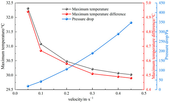
Figure 12.
Influence of different inlet velocity on Tmax, ΔTmax, and ΔP.
4.2.3. Influence of Different Channel Depths
The variation in performance is explored as the channel depth increases from 5 mm to 3.5 mm, with eight branch channels, an inlet velocity of 0.1 m·s−1, a channel width of 3 mm, and a channel angle of 60°. The variation curves of the Tmax, ΔTmax, and ΔP with the channel depth are shown in Figure 13. With the increase in channel depth, the Tmax, ΔTmax, and ΔP all decrease, and the slopes of the corresponding curves decrease gradually. It is indicated that the cooling performance of the liquid cooling plate improves with increasing channel depth, but the improvement gradually flattens. The reason is that as the channel depth increases, the heat exchange area at the interface between the coolant fluid domain and the cooling plate solid domain increases, allowing the heat generated by the battery to be transferred to the coolant more promptly and effectively, thereby improving the overall heat dissipation performance.
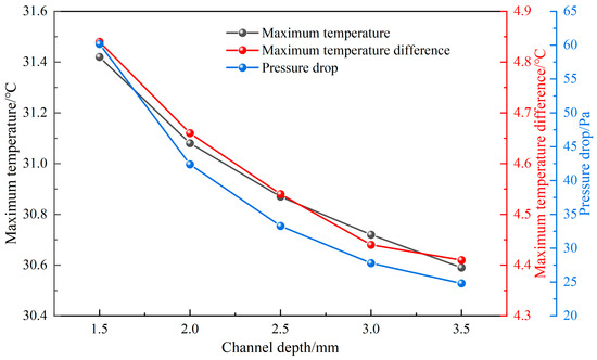
Figure 13.
Influence of different channel depths on Tmax, ΔTmax, and ΔP.
4.2.4. Influence of Different Channel Widths
The variation in performance is explored as the channel width increases from 2 mm to 6 mm, with eight branch channels, an inlet velocity of 0.1 m·s−1, a channel depth of 2 mm, and a channel angle of 60°. The variation curves of the Tmax, ΔTmax, and ΔP with the channel width are shown in Figure 14. As the channel width increases, both the Tmax and ΔTmax decrease accordingly. When the channel width is 2 mm, the Tmax is 31.18 °C and the ΔTmax is 4.7 °C. When the channel width is 6 mm, the Tmax is 30.92 °C and the ΔTmax is 4.57 °C. The increased channel width enhances the heat exchange area between the coolant and the liquid cooling plate, thereby improving the cooling performance of the liquid cooling plate. The ΔP decreases from 54.7 Pa to 31.04 Pa, indicating that increasing the channel width helps reduce the ΔP and achieve lower power consumption.
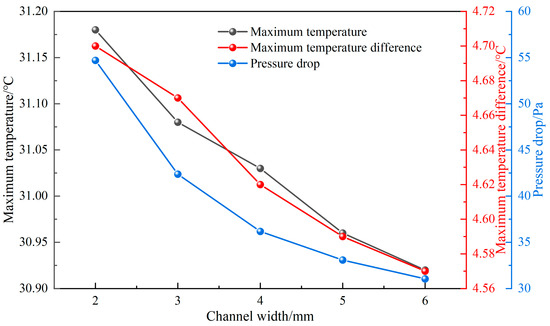
Figure 14.
Influence of different channel widths on Tmax, ΔTmax, and ΔP.
4.2.5. Influence of Different Channel Angles
The variation in performance is explored as the channel angle increases from 60° to 80°, with eight branch channels, an inlet velocity of 0.1 m·s−1, a channel depth of 2 mm, and a channel width of 3 mm. The variation curves of the Tmax, ΔTmax, and ΔP with the channel angle are shown in Figure 15. As the channel angle increases from 60° to 80°, there is a slight decrease in the Tmax from 31.08 °C to 31.03 °C and a small reduction in the ΔTmax from 4.67 °C to 4.62 °C. This is attributed to the more uniform distribution of channels within the cooling plate, resulting in a slightly enhanced heat transfer efficiency for the cooling plate. Additionally, as the channel angle increases, the ΔP increases slightly from 42.38 Pa to 43.22 Pa.
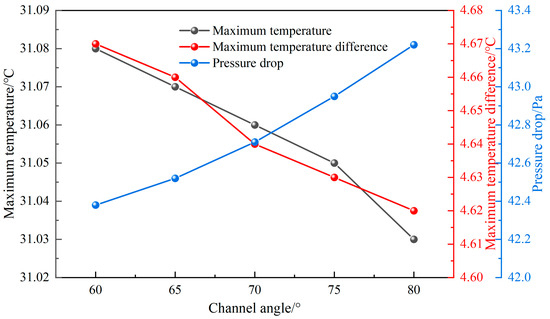
Figure 15.
Influence of different channel angles on Tmax, ΔTmax, and ΔP.
4.3. Sensitivity Analysis of Different Factors
The sensitivity analysis of diverse variables is conducted to identify those with significant influence. The formula for calculating the sensitivity factor SAi is as follows [39].
where fmax(xi) and fmin(xi) are the maximum and minimum objective values.
The results of the sensitivity analysis are shown in Figure 16. It can be observed that the flow velocity has the greatest impact on the three objectives, particularly on the ΔP, with a sensitivity factor as high as 86.53%. This is primarily attributed to the fact that the pressure loss of coolant is directly proportional to the square of the flow velocity, so an increase in flow velocity significantly raises the ΔP. In contrast, the channel angle has the least impact on the three objectives, especially on the ΔP, with a sensitivity factor of only 0.22%. As such, changing the channel angle has a very limited influence on the three objectives. After comprehensive consideration, the channel depth, channel width, and flow velocity are selected as the input variables for multi-objective optimization.
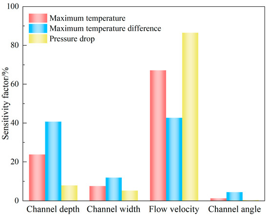
Figure 16.
Sensitivity factors for the different variables.
4.4. Analysis of Prediction Results
4.4.1. Model Performance Evaluation
The prediction performance of the model is assessed using the correlation coefficient (R2), mean absolute error (MAE), and root mean square error (RMSE). The corresponding equations are shown below:
where yi is the simulated value, is the predicted value, is the average of the simulated values, and n is the number of test samples.
4.4.2. Analysis of Prediction Results on the Training Set
The optimal fitness variation curve of the PSO algorithm is depicted in Figure 17a. During the iterative process, the particle swarm gradually moves towards the optimal fitness value as a whole. In the first six iterations, the fitness value decreases significantly. After the sixth iterations, the fitness value changes little, with the optimization curve gradually converging. Once the preset 50 iterations are completed, the optimization process automatically terminates and outputs the optimal results. The optimal parameter combination obtained from the search is then substituted into the BPNN model for training to assess the prediction performance of the PSO-BPNN model on the previously designated 80% training set. Figure 17b–d shows the comparison between the predicted values and the true values for three objectives in the training set. It is clearly demonstrated by these figures that the prediction results for the training set are quite good, indicating that the PSO-BPNN model can effectively fit the training data. This further proves that the model possesses excellent multi-input and multi-output nonlinear fitting capabilities, thus qualifying it as a surrogate model for subsequent prediction validation on the test set.
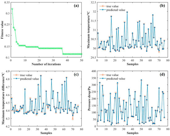
Figure 17.
(a) Optimal fitness variation with iterations in the PSO algorithm, (b) Tmax prediction curve, (c) ΔTmax prediction curve, and (d) ΔP prediction curve.
4.4.3. Analysis of Prediction Results on the Test Set
To confirm the efficiency of using the PSO algorithm, the prediction results on the test set are compared between the BPNN and the PSO-BPNN models. The comparison of the prediction results for the two models is shown in Figure 18, and the comparison of relevant evaluation metrics is presented in Table 5. Specifically, Figure 18a,c,e compares the true values with the predicted values for the PSO-BPNN model, while Figure 18b,d,f shows the same comparisons for the traditional BPNN model. As evident from the figure and table, the prediction results of the three objectives based on the PSO-BPNN model are closer to the true values compared to those of the traditional BPNN model. The errors of various evaluation metrics in the prediction results using the PSO-BPNN model are all smaller than those of the traditional BPNN model, while the R2 values are higher. For the third objective of ΔP, the RMSE and MAE are improved by 51.5% and 55.5%, respectively. This demonstrates that optimizing the number of hidden nodes, learning rate, initial weights, and initial thresholds of the BPNN using the PSO algorithm significantly enhances the prediction accuracy of the model, thus offering higher application value.
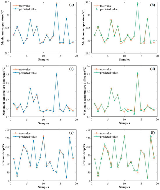
Figure 18.
(a) Tmax prediction curve in the PSO-BPNN, (b) Tmax prediction curve in the BPNN, (c) ΔTmax prediction curve in the PSO-BPNN, (d) ΔTmax prediction curve in the BPNN, (e) ΔP prediction curve in the PSO-BPNN, (f) ΔP prediction curve in the BPNN.
Table 5.
Comparison of the evaluation metrics between the two models.
4.5. Multi-Objective Optimization
The NSGA-II algorithm is employed with the following parameter settings: an initial population of 100 individuals, a total of 200 iterations, a crossover probability of 0.8, and a mutation probability of 0.1. After 200 generations of iterative calculations, a smooth curve composed of the Pareto solutions is finally obtained. As can be seen in Figure 19, the Pareto solutions are mutually restrictive, such that a decrease in the Tmax and ΔTmax leads to an increase in ΔP. As such, these three objectives cannot be minimized simultaneously. The Pareto front curve exhibits a convex trend towards the lower left corner, demonstrating good uniformity and distribution.
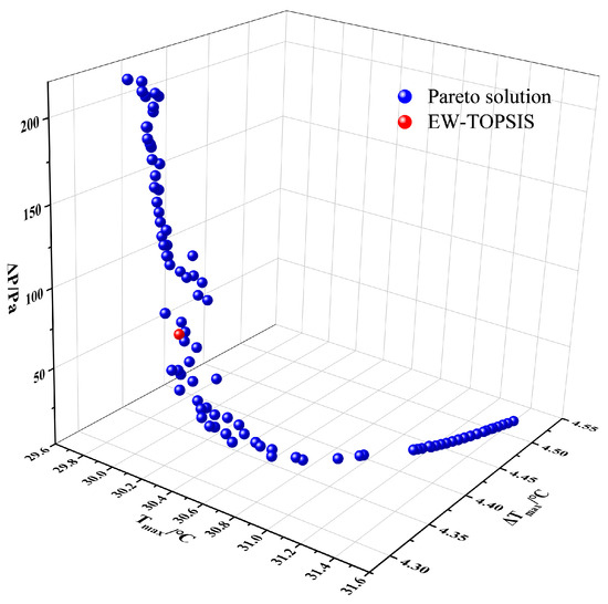
Figure 19.
Pareto optimal solution set.
Each individual on the Pareto front is non-dominated, so it is necessary to comprehensively consider the three objectives to select an optimal solution from the Pareto front. In the actual selection process, decisions often rely on experience and personal preferences. Typically, the optimal solution is selected based on the Pareto front curve, with a tendency to choose points in the middle of the curve to balance the various optimization objectives. However, this approach is subjective and makes it difficult to ensure that the optimal solution is obtained. To address this issue, the entropy weight method is utilized to determine the weight of each objective, and then the TOPSIS method is used to objectively select the optimal solution.
4.6. Optimization Results of the Entropy Weight–TOPSIS Method
With the entropy weight results for the three objectives presented in Table 6, the weights for the Tmax, ΔTmax, and ΔP are 0.498, 0.225, and 0.277, respectively. Among them, the objective of Tmax holds the highest weight, while the objective of ΔTmax has the lowest weight. Based on the determined weights of the three objectives, the TOPSIS method is utilized to evaluate the performance of various combinations of variable parameters. When the channel width, channel depth, and inlet velocity are set to 6 mm, 3.4 mm, and 0.22 m·s−1, respectively, the overall performance of the liquid cooling plate reaches its optimum. To verify the reliability of the multi-objective optimization results, simulations are conducted on the optimized flow channel, and the results are compared with those obtained from the optimization process. As shown in Table 7, the optimization values of the three objectives differ minimally from the simulation values, demonstrating that the multi-objective optimization results are reliable. Compared to the initial structure, although the ΔP in the optimized structure increases by 21.24 Pa, the Tmax and ΔTmax are reduced by 1.09 °C and 0.41 °C, respectively. The temperature contour plots of the batteries in the initial and optimized structures are shown in Figure 20. It is evident that the Tmax of the batteries decreases, along with a more uniform temperature distribution in the optimized structure. The thermal simulation results of the battery module incorporating the optimized structure are supplied in Appendix A, showcasing the superior cooling performance in comparison with the straight and serpentine structures.
Table 6.
Entropy weight results of the three objectives.
Table 7.
Comparison of calculation results.
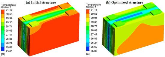
Figure 20.
Temperature contour plots of the batteries: (a) the initial structure, (b) the optimized structure.
5. Conclusions
In this paper, a PSO-BPNN surrogate model is proposed to predict the cooling performance of the spider-web liquid cooling plate. The channel width, channel depth, and inlet velocity are selected as optimization variables, while the Tmax, ΔTmax, and ΔP are the optimization objectives. Based on the surrogate model, the NSGA-II algorithm is employed to optimize the variables and obtain the Pareto solution set. The optimal solution is selected by the TOPSIS with entropy weight method. The major conclusions are summarized as follows:
(1) Compared to conventional straight and serpentine flow channels, the spider-web flow channel demonstrates superior cooling performance and has a smaller ΔP than the other two channel types. The channel depth and inlet velocity are the primary factors influencing the cooling performance of the spider-web flow channel, while the channel angle has a relatively minor impact.
(2) Based on the sample point data obtained through OLHS, a PSO-BPNN surrogate model is established to predict the cooling performance of the spider-web liquid cooling plate. The results indicate that the PSO-BPNN model exhibits superior performance in prediction accuracy, as evidenced by lower MAE and RMSE values and a higher R2 value.
(3) By applying the entropy weight method, the weights for the Tmax, ΔTmax, and ΔP are 0.498, 0.225, and 0.277, respectively. Based on these weights and the TOPSIS decision-making method, a good balance between cooling performance and energy consumption is achieved when the channel width, channel depth, and inlet velocity are 6 mm, 3.4 mm, and 0.22 m·s−1, respectively. Compared to the initial structure, the Tmax and ΔTmax are reduced by 1.09 °C and 0.41 °C in the optimized structure, respectively, with an increase in ΔP by 21.24 Pa.
Author Contributions
Investigation and writing—original draft, J.L.; methodology, J.L. and H.Z.; writing—review and editing, J.L., H.Z., W.Y. and Y.Z.; conceptualization, supervision, and funding acquisition, H.Z. All authors have read and agreed to the published version of the manuscript.
Funding
This research was funded by the National Natural Science Foundation of China (52476079).
Data Availability Statement
Data will be made available on request.
Conflicts of Interest
Author Yapeng Zhou was employed by the China Merchants Testing Vehicle Technology Research Institute Limited Company. The remaining authors declare that the research was conducted in the absence of any commercial or financial relationships that could be construed as a potential conflict of interest.
Nomenclature/Abbreviations
| Nomenclature | |
| c | specific heat capacity/J·kg−1·K−1 |
| D | hydraulic diameter/m |
| G | coefficient of variation |
| h | convective heat transfer coefficient/W·m−2·K−1 |
| ΔP | pressure drop/Pa |
| q | volumetric heat generation rate/W·m−3 |
| S | entropy value |
| T | temperature/°C |
| Tmax | maximum temperature/°C |
| ΔTmax | maximum temperature difference/°C |
| v | velocity/m·s−1 |
| Greek letters | |
| ρ | density/kg·m−3 |
| λ | thermal conductivity/W·m−1·K−1 |
| μ | dynamic viscosity/Pa·s |
| ∇2 | laplacian operator |
| Subscripts | |
| a | ambient |
| bat | battery |
| f | fluid |
| lcp | liquid cooling plate |
| sur | surface |
| Abbreviations | |
| BPNN | back propagation neural network |
| BTMS | battery thermal management system |
| EW | entropy weight |
| MAE | mean absolute error |
| NSGA-II | non-dominated sorting genetic algorithm II |
| OLHS | optimal Latin hypercube sampling |
| PCM | phase change material |
| PSO | particle swarm optimization |
| R2 | correlation coefficient |
| RMSE | root mean square error |
| TOPSIS | technique for order preference by similarity to an ideal solution |
| UDF | user defined function |
Appendix A
To demonstrate the cooling performance difference between the normal liquid cooling plates and the optimized spider-web liquid cooling plate. The temperature contour plots of the battery module are shown in Figure A1. The optimized spider-web liquid cooling plate has superior cooling performance, with the Tmax of the battery module reaching 28.17 °C and the ΔTmax of 2.53 °C. Compared to the serpentine and straight liquid cooling plates, the Tmax decreased by 0.69 °C (17.9%) and 0.54 °C (14.6%), respectively, while the ΔTmax decreased by 0.4 °C (13.7%) and 0.35 °C (12.2%). As such, the optimized spider-web liquid cooling plate is also applicable for module cooling.
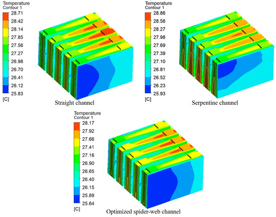
Figure A1.
Temperature contour plots of the battery module.
References
- Xiong, R.; Pan, Y.; Shen, W.; Li, H.; Sun, F. Lithium-ion battery aging mechanisms and diagnosis method for automotive applications: Recent advances and perspectives. Renew. Sustain. Energy Rev. 2020, 131, 110048. [Google Scholar] [CrossRef]
- Zhang, X.; Li, Z.; Luo, L.; Fan, Y.; Du, Z. A review on thermal management of lithium-ion batteries for electric vehicles. Energy 2022, 238, 121652. [Google Scholar] [CrossRef]
- Huang, Y.; Tang, Y.; Yuan, W.; Fang, G.; Yang, Y.; Zhang, X.; Wu, Y.; Yuan, Y.; Wang, C.; Li, J. Challenges and recent progress in thermal management with heat pipes for lithium-ion power batteries in electric vehicles. Sci. China Technol. Sci. 2021, 64, 919–956. [Google Scholar] [CrossRef]
- Nazari, A.; Farhad, S. Heat generation in lithium-ion batteries with different nominal capacities and chemistries. Appl. Therm. Eng. 2017, 125, 1501–1517. [Google Scholar] [CrossRef]
- Monika, K.; Datta, S. Comparative assessment among several channel designs with constant volume for cooling of pouch-type battery module. Energy Convers. Manag. 2022, 251, 114936. [Google Scholar] [CrossRef]
- Khoshvaght-Aliabadi, M.; Abbaszadeh, A.; Salimi, A.; Salehi, N. Structural modifications of sinusoidal wavy minichannels cold plates applied in liquid cooling of lithium-ion batteries. J. Energy Storage 2023, 57, 106208. [Google Scholar] [CrossRef]
- Zhang, Y.; Cheng, S.; Mei, W.; Jiang, L.; Jia, Z.; Cheng, Z.; Sun, J.; Wang, Q. Understanding of thermal runaway mechanism of LiFePO4 battery in-depth by three-level analysis. Appl. Energy 2023, 336, 120695. [Google Scholar] [CrossRef]
- Wang, C.; Xu, J.; Wang, M.; Xi, H. Experimental investigation on reciprocating air-cooling strategy of battery thermal management system. J. Energy Storage 2023, 58, 106406. [Google Scholar] [CrossRef]
- Wang, M.; Teng, S.; Xi, H.; Li, Y. Cooling performance optimization of air-cooled battery thermal management system. Appl. Therm. Eng. 2021, 195, 117242. [Google Scholar] [CrossRef]
- Wang, C.; Zhang, G.; Li, X.; Huang, J.; Wang, Z.; Lv, Y.; Meng, L.; Situ, W.; Rao, M. Experimental examination of large capacity LiFePO4 battery pack at high temperature and rapid discharge using novel liquid cooling strategy. Int. J. Energy Res. 2018, 42, 1172–1182. [Google Scholar] [CrossRef]
- Zhao, D.; Lei, Z.; An, C. Research on battery thermal management system based on liquid cooling plate with honeycomb-like flow channel. Appl. Therm. Eng. 2023, 218, 119324. [Google Scholar] [CrossRef]
- Wang, X.; Xie, Y.; Day, R.; Wu, H.; Hu, Z.; Zhu, J.; Wen, D. Performance analysis of a novel thermal management system with composite phase change material for a lithium-ion battery pack. Energy 2018, 156, 154–168. [Google Scholar] [CrossRef]
- Al-Abidi, A.; Mat, S.; Sopian, K.; Sulaiman, M.; Mohammad, A. Numerical study of PCM solidification in a triplex tube heat exchanger with internal and external fins. Int. J. Heat Mass Transf. 2013, 61, 684–695. [Google Scholar] [CrossRef]
- Mbulu, H.; Laoonual, Y.; Wongwises, S. Experimental study on the thermal performance of a battery thermal management system using heat pipes. Case Stud. Therm. Eng. 2021, 26, 101029. [Google Scholar] [CrossRef]
- Smith, J.; Singh, R.; Hinterberger, M.; Mochizuki, M. Battery thermal management system for electric vehicle using heat pipes. Int. J. Therm. Sci. 2018, 134, 517–529. [Google Scholar] [CrossRef]
- Chen, K.; Wang, S.; Song, M.; Chen, L. Structure optimization of parallel air-cooled battery thermal management system. Int. J. Heat Mass Transf. 2017, 111, 943–952. [Google Scholar] [CrossRef]
- Yan, J.; Wang, Q.; Li, K.; Sun, J. Numerical study on the thermal performance of a composite board in battery thermal management system. Appl. Therm. Eng. 2016, 106, 131–140. [Google Scholar] [CrossRef]
- Li, W.; Qu, Z.; He, Y.; Tao, W. Experimental and numerical studies on melting phase change heat transfer in open-cell metallic foams filled with paraffin. Appl. Therm. Eng. 2012, 37, 1–9. [Google Scholar] [CrossRef]
- Zhang, Z.; Wei, K. Experimental and numerical study of a passive thermal management system using flat heat pipes for lithium-ion batteries. Appl. Therm. Eng. 2020, 166, 114660. [Google Scholar] [CrossRef]
- Xia, G.; Cao, L.; Bi, G. A review on battery thermal management in electric vehicle application. J. Power Sources 2017, 367, 90–105. [Google Scholar] [CrossRef]
- Tan, X.; Lyu, P.; Fan, Y.; Rao, J.; Ouyang, K. Numerical investigation of the direct liquid cooling of a fast-charging lithium-ion battery pack in hydrofluoroether. Appl. Therm. Eng. 2021, 196, 117279. [Google Scholar] [CrossRef]
- Wang, H.; Tao, T.; Xu, J.; Shi, H.; Mei, X.; Gou, P. Thermal performance of a liquid-immersed battery thermal management system for lithium-ion pouch batteries. J. Energy Storage 2022, 46, 103835. [Google Scholar] [CrossRef]
- Li, X.; Zhao, J.; Duan, J.; Panchal, S.; Yuan, J.; Fraser, R.; Fowler, M.; Chen, M. Simulation of cooling plate effect on a battery module with different channel arrangement. J. Energy Storage 2022, 49, 104113. [Google Scholar] [CrossRef]
- Sheng, L.; Su, L.; Zhang, H.; Li, K.; Fang, Y.; Ye, W.; Fang, Y. Numerical investigation on a lithium-ion battery thermal management utilizing a serpentine-channel liquid cooling plate exchanger. Int. J. Heat Mass Transf. 2019, 41, 658–668. [Google Scholar] [CrossRef]
- Huang, Y.; Mei, P.; Lu, Y.; Huang, R.; Yu, X.; Chen, Z.; Roskilly, A. A novel approach for Lithium-ion battery thermal management with streamline shape mini channel cooling plates. Appl. Therm. Eng. 2019, 157, 113623. [Google Scholar] [CrossRef]
- Wang, Y.; Xu, X.; Liu, Z.; Kong, J.; Zhai, Q.; Zakaria, H.; Wang, Q.; Zhou, F.; Wei, H. Optimization of liquid cooling for prismatic battery with novel cold plate based on butterfly-shaped channel. J. Energy Storage 2023, 73, 109161. [Google Scholar] [CrossRef]
- Liu, F.; Chen, Y.; Qin, W.; Li, J. Optimal design of liquid cooling structure with bionic leaf vein branch channel for power battery. Appl. Therm. Eng. 2023, 218, 119283. [Google Scholar] [CrossRef]
- Fan, X.; Meng, C.; Yang, Y.; Lin, J.; Li, W.; Zhao, Y.; Xie, S.; Jiang, C. Numerical optimization of the cooling effect of a bionic fishbone channel liquid cooling plate for a large prismatic lithium-ion battery pack with high discharge rate. J. Energy Storage 2023, 72, 108239. [Google Scholar] [CrossRef]
- Li, A.; Yuen, A.; Wang, W.; Weng, J.; Yeoh, G. Numerical investigation on the thermal management of lithium-ion battery system and cooling effect optimization. Appl. Therm. Eng. 2022, 215, 118966. [Google Scholar] [CrossRef]
- Chen, Y.; Li, D.; Feng, S.; Huang, Q.; Chen, Z.; Shu, D. Optimization and thermal-performance deep learning on carbon/epoxy composite panels with microchannel structure for battery cooling. Appl. Therm. Eng. 2022, 217, 119162. [Google Scholar] [CrossRef]
- Ding, Y.; Ji, H.; Wei, M.; Liu, R. Effect of liquid cooling system structure on lithium-ion battery pack temperature fields. Int. J. Heat Mass Transf. 2022, 183, 122178. [Google Scholar] [CrossRef]
- Shen, K.; Sun, J.; Zheng, Y.; Xu, C.; Wang, H.; Wang, S.; Chen, S.; Feng, X. A comprehensive analysis and experimental investigation for the thermal management of cell-to-pack battery system. Appl. Therm. Eng. 2022, 211, 118422. [Google Scholar] [CrossRef]
- Monika, K.; Chakraborty, C.; Roy, S.; Dinda, S.; Singh, S.; Datta, S. An improved mini-channel based liquid cooling strategy of prismatic LiFePO4 batteries for electric or hybrid vehicles. J. Energy Storage 2021, 35, 102301. [Google Scholar] [CrossRef]
- Xin, Q.; Yang, T.; Zhang, H.; Yang, J.; Zeng, J.; Xiao, J. Experimental and numerical study of lithium-ion battery thermal management system using composite phase change material and liquid cooling. J. Energy Storage 2023, 71, 108003. [Google Scholar] [CrossRef]
- Peng, Y.; Zhou, J.; Hou, L.; Wang, K.; Chen, C.; Zhang, H. A hybrid MCDM-based optimization method for cutting-type energy-absorbing structures of subway vehicles. Struct. Multidisc. Optim. 2022, 65, 228. [Google Scholar] [CrossRef]
- Mason, K.; Duggan, J.; Howley, E. Multi-objective dynamic economic emission dispatch using particle swarm optimization variants. Neurocomputing 2017, 270, 188–197. [Google Scholar] [CrossRef]
- He, Y.; Guo, H.; Jin, M.; Ren, P. A linguistic entropy weight method and its application in linguistic multi-attribute group decision making. Nonlinear Dyn. 2016, 84, 399–404. [Google Scholar] [CrossRef]
- Li, Y.; Kong, B.; Qiu, C.; Li, Y.; Jiang, Y. Numerical study on air-cooled battery thermal management system considering the sheer altitude effect. Appl. Therm. Eng. 2025, 258, 124707. [Google Scholar] [CrossRef]
- Chen, S.; Peng, X.; Bao, N.; Garg, A. A comprehensive analysis and optimization process for an integrated liquid cooling plate for a prismatic lithium-ion battery module. Appl. Therm. Eng. 2019, 156, 324–339. [Google Scholar] [CrossRef]
Disclaimer/Publisher’s Note: The statements, opinions and data contained in all publications are solely those of the individual author(s) and contributor(s) and not of MDPI and/or the editor(s). MDPI and/or the editor(s) disclaim responsibility for any injury to people or property resulting from any ideas, methods, instructions or products referred to in the content. |
© 2025 by the authors. Licensee MDPI, Basel, Switzerland. This article is an open access article distributed under the terms and conditions of the Creative Commons Attribution (CC BY) license (https://creativecommons.org/licenses/by/4.0/).