State of Health Estimation for Lithium-Ion Batteries Based on Transition Frequency’s Impedance and Other Impedance Features with Correlation Analysis

Abstract

This paper presents data-driven impedance-based state of health (SOH) estimation for commercial lithium-ion batteries across an SOH range of ~96% to ~60%. Battery health indicators at the transition frequency of the battery impedance Nyquist plot are utilized to develop an SOH estimator based on an artificial neural network (ANN). In addition, two more ANN-based SOH estimators utilizing some impedance magnitude and phase values are developed. Spearman correlation analysis is utilized to identify the frequency points at which the impedance magnitude and phase values show strong correlations with SOH values and are thus utilized as SOH indicators. The performance evaluation of the developed SOH estimators shows that the maximum root mean square error (RMSE) is equal to 1.39%, the maximum mean absolute error (MAE) is equal to 1.25%, the maximum mean absolute percentage error (MAPE) is equal to 1.55%, and the minimum coefficient of determination (R²) is equal to 0.983.

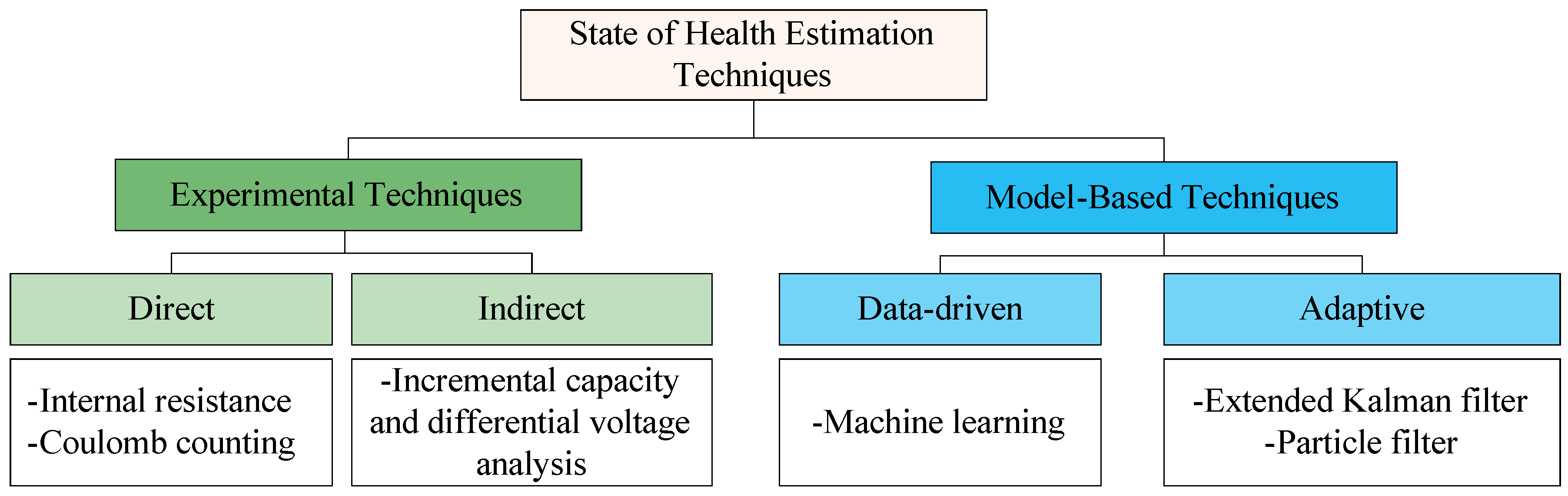
1. Introduction

Lithium-ion batteries have been widely adopted across a range of applications, from electric vehicles (EVs) to consumer electronics, owing to several advantages such as high energy density and low internal discharge [1]. To meet the increasing performance requirements of battery packs, developing advanced battery management systems (BMS) has become an essential step. One of the most important BMS functions is the state of health (SOH) estimation [2,3,4,5,6]. Battery SOH estimation is crucial in prolonging the lifetime of battery systems and maintaining their safety. SOH estimation is utilized in monitoring the health of the battery, suggesting better battery charging and discharging strategies, and triggering protection functions to avoid battery failures. Recently, SOH estimation gained more attention in second-use (i.e., retired) battery applications. In such applications, SOH estimation is essential for the safe and efficient utilization of second-use batteries [7,8,9].

Battery aging (i.e., health deterioration) causes include, but are not limited to, high/low temperature outside normal range, over/under voltage, and mechanical stress [10]. Battery aging types can be classified into calendar aging and cyclic aging [10]. Calendar aging is due to side reactions while the battery is not in use, whereas cyclic aging is due to repeated battery charging and discharging (cycling). Several mechanisms govern battery aging, such as solid electrolyte interface (SEI) formation and thickening, cathode electrolyte interface (CEI) formation, lithium plating, and binder decomposition [11]. Generally, battery health degradation appears as power fade and capacity fade. In terms of capacity fade, the SOH value for a battery can be defined as the ratio between the available capacity Q_available and the nominal capacity Q_nominal as expressed in (1):

$$SOH=Q_{\mathrm{a}\mathrm{v}\mathrm{a}\mathrm{i}\mathrm{l}\mathrm{a}\mathrm{b}\mathrm{l}\mathrm{e}}/Q_{\mathrm{n}\mathrm{o}\mathrm{m}\mathrm{i}\mathrm{n}\mathrm{a}\mathrm{l}}$$

(1)

where the available capacity Q_available is the amount of charge that a fully charged battery can provide when the battery is discharged to its minimum voltage, where Q_nominal is provided by the manufacturer.

Many SOH estimation techniques were proposed in the literature with various classifications [5,6,9,12,13,14,15,16,17]. The classifications are based on different factors such as the variables needed to estimate the SOH, the need for direct measurement, and whether circuit and/or physical models are utilized or not. Generally, SOH estimation techniques can be classified into experimental techniques and model-based techniques, as illustrated in Figure 1. The white boxes at the bottom of Figure 1 include examples for each SOH estimation category/subcategory.

Experimental techniques can be direct or indirect. Examples of direct techniques include utilizing the internal resistance and Coulomb counting to estimate the SOH. The internal resistance is affected by battery aging in such a way that its value increases as the battery ages (i.e., as the SOH value decreases) [18]. The current pulse method [19,20] is usually utilized to estimate the internal resistance. However, the internal resistance of a battery is a function of various factors such as temperature and state of charge (SOC) [21,22]. The Coulomb counting method is based on counting the Ampere-Hour (Ah) during battery discharging and charging. The Ah amount supplied/accepted by the battery during discharging/charging changes as the battery ages [3]. Despite its simplicity, the Coulomb counting method suffers from sensing error accumulation [23].

Incremental capacity (i.e., the derivative of the accumulated capacity during a charge/discharge process with respect to voltage, referred to as “IC”) and differential voltage (dV) analyses utilize the relationship between the incremental capacity and the battery voltage to indirectly identify aging patterns and estimate the SOH value; for example, by utilizing the peaks in the voltage–IC curves [24,25].

Model-based techniques utilize various models to estimate the SOH value of a battery, and they are classified into adaptive and data-driven techniques. Adaptive SOH techniques are capable of adjusting and updating their parameters based on data obtained from real-time operation. Some examples of adaptive techniques include the Kalman filter [26,27,28] and particle filter [29,30,31].

Data-driven SOH estimation techniques have gained more interest over the past decade, especially with the advancements in computation capabilities. Without a need to know the underlying aging mechanisms, data-driven techniques capture aging patterns and extract features from battery historical data [3,32,33].

SOH estimation based on the battery impedance has drawn attention in the literature due to its speed and ability to reflect the battery’s internal electrochemical processes [33,34]. Generally, SOH features are extracted from the impedance curves (the impedance magnitude, phase, and Nyquist). Utilizing battery impedance for SOH estimation might fall into one of the following three categories:

(1)

Utilizing a broadband EIS curve to estimate the SOH value. The authors in [35] utilized the entire EIS curve of 60 frequency points (120 points of 60 real impedance values and 60 imaginary impedance values) to predict the SOH. However, this study was for 45 mAh coin cell batteries. Also, utilizing a high-dimensional input increases the computational cost.

(2)

Identifying specific points from the impedance curves to be utilized as SOH features:

• Fixed-frequency impedance points: impedance values at specific frequencies are identified to have a strong correlation with the SOH value, such as the impedance magnitude at 1 kHz [36] and 316 Hz [37]; impedance real part at 0.1 Hz [38]; and the impedance imaginary part at 17.8 Hz and 2.16 Hz [35].
• Non-fixed frequency points: features are identified from the pattern at which the impedance curves change at different SOH values, such as the minimum impedance magnitude [39], the impedance magnitude when the impedance phase is equal to 0° [33], and the value of the frequency at which the impedance phase is equal to 0° [40].
• Features from the Nyquist plot (the plot of the impedance real part against the impedance imaginary part): By studying how Nyquist plots change with SOH, various features can be extracted to be utilized for SOH estimation. For example, at the Nyquist plot’s peak point, the impedance real part, the impedance imaginary part, and the impedance vector amplitude were utilized for SOH estimation in [21].
• Features from the phase–magnitude plot: Another way to look at the battery’s impedance spectrum is to plot the phase against the magnitude [34]. From the phase–magnitude plot, some SOH features can be obtained, such as the differential impedance magnitude, which is the difference in the impedance magnitude at the valley and peak of the phase–magnitude plot [34].

(3)

Fitting the EIS curve to obtain values for the equivalent circuit model (ECM) parameters. For example, the EIS curve can be fit to obtain values for solid electrolyte interphase (SEI) resistance [41,42], diffusion constant phase elements [43], and charge transfer resistance [44]. The change in the ECM parameters is utilized for SOH estimation.

This paper contributes to different categories of those mentioned above by presenting different SOH estimators. First, an SOH estimator is developed based on the battery’s real and imaginary impedance parts at the transition frequency within the impedance Nyquist plot (contributing to category 2.c from the categories above). Second, this paper contributes to category 2.a from the categories above by presenting two more SOH estimators: one utilizing features extracted from the impedance magnitude curve, and another utilizing features extracted from the impedance phase curve (that is not common in the literature). A correlation analysis is carried out to identify the frequency points at which the impedance magnitude and phase are utilized as indicators for SOH estimation. The performance of the developed SOH estimators is evaluated along with some insights. The batteries used in this paper were deeply aged to a highly deteriorated SOH value (~60%), which fills a gap in the literature for EIS data of batteries under deep degradation levels. The remainder of this paper is organized as follows: Section 2 introduces the battery aging and data collection protocol followed to obtain aging data needed for SOH estimation model training and testing. Section 3 presents the proposed SOH indicators for each estimator. Section 4 presents a correlation analysis to identify the key frequency range (or points) for impedance points (magnitude and phase) to be used in SOH estimators. Section 5 presents the SOH estimation model and its accuracy evaluation. Finally, the conclusions are drawn in Section 6.

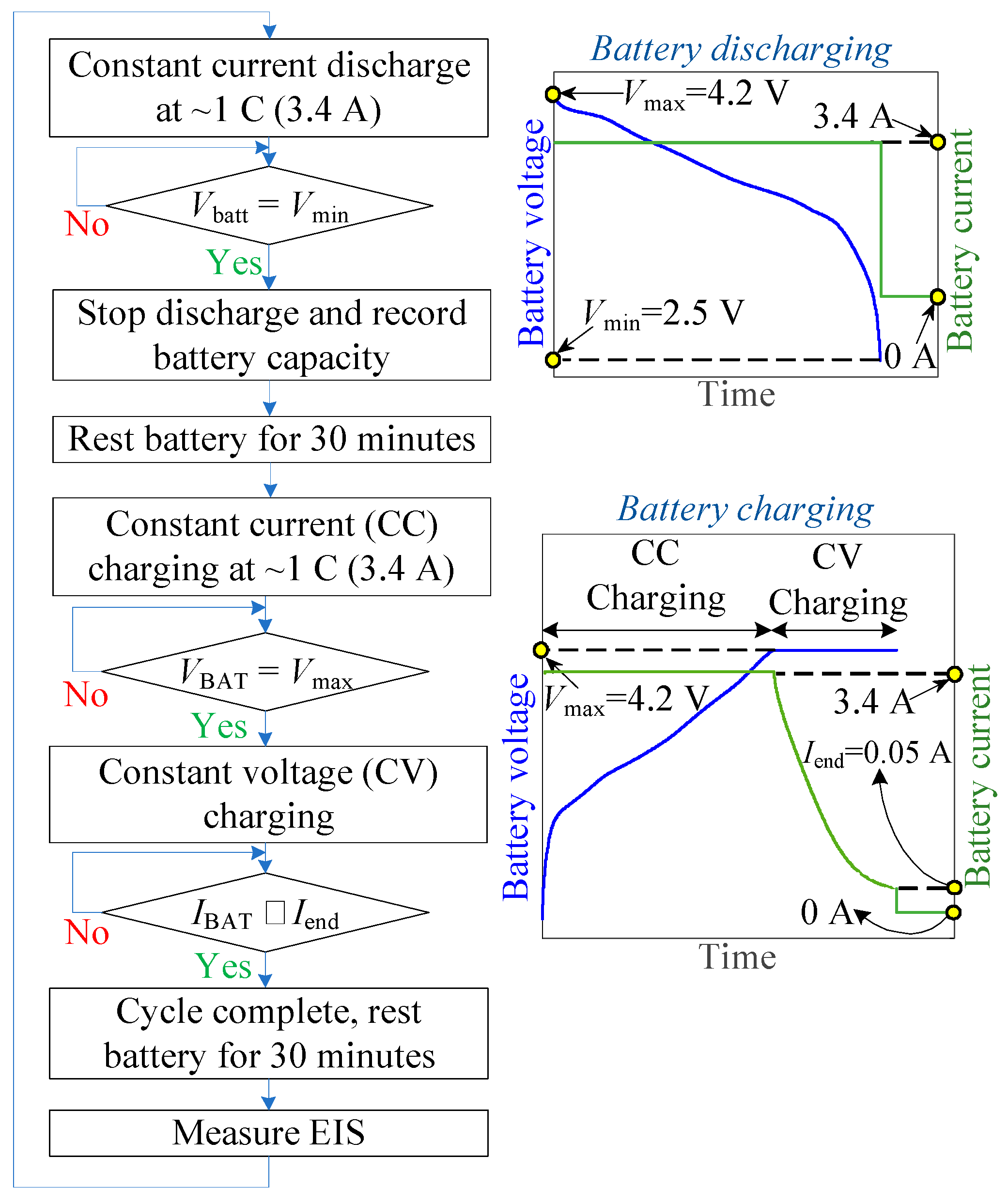
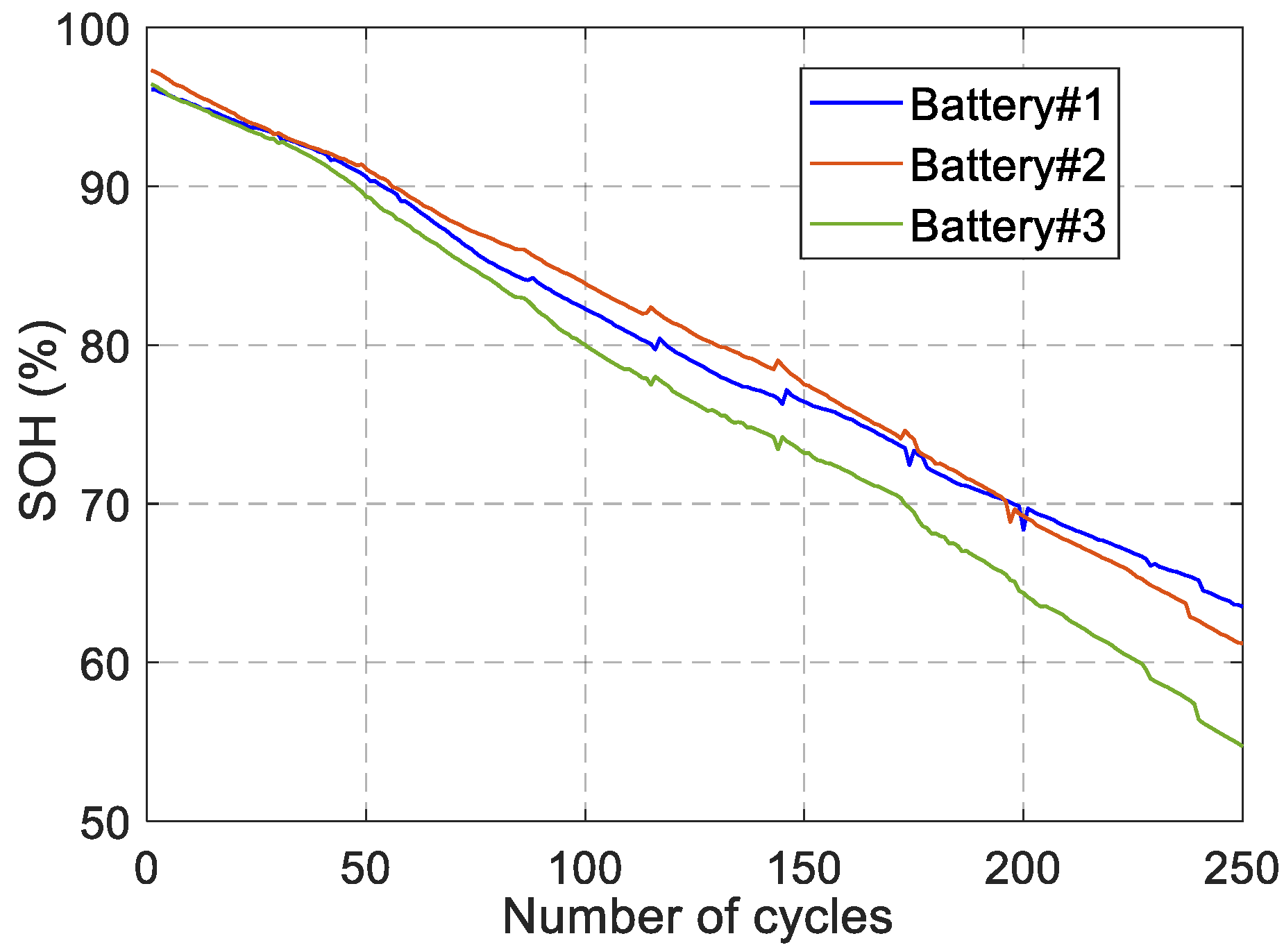
2. Battery Aging and Data Collection Protocol

Three commercial LG INR18650 3500 mAh battery cells (by LG Chem Ltd., Seoul, Republic of Korea) [45] were cycled/aged in the laboratory according to the aging protocol shown in Figure 2.

The main manufacturer’s specifications for the cycled battery cells are listed in

Table 1. Main manufacturer’s specifications for LG INR18650MJ1-3.5Ah battery cell [45].

Nominal capacity C	3.5 Ah
Nominal voltage Vnom	3.635 V
Minimum voltage Vmin	2.50 V
Maximum voltage Vmax	4.2 V
Maximum charging current	3.4 A
Charing end current Iend	0.05 A

[45]. Before cycling the battery cells, the initial capacity of each battery cell is calibrated using the Coulomb counting method by fully discharging the battery. Also, the EIS curve is measured for each battery cell to obtain the SOH features at the initial capacity level (the initial SOH value). Then, each battery cell undergoes a cycling process in which the battery cell is repeatedly discharged and charged. The battery cell is discharged at ~1 C (3.4 A). The battery cell discharging operation is utilized to measure the battery capacity at each cycle using the Coulomb counting method by integrating the battery discharge current over time during the discharging operation in each cycle. Battery cell charging starts with constant current (CC) charging mode in which the charging current is regulated at ~1 C (3.4 A). Once the battery cell voltage reaches the maximum value (i.e., 4.2 V for the battery cells used in this paper), the constant voltage (CV) charging mode starts by regulating the battery voltage at 4.2 V until the battery current drops below the charging end current I_end (0.05 A for the battery cells used in this paper). The battery cell is rested for 30 min after each discharge operation and after each charge operation. The battery cells were cycled at room temperature (~23 °C) with a relative humidity in the range of 40–60%. Battery cell cycling and EIS measurements were carried out using the Squidstat Cycler—Base Model from Admiral Instruments (main specifications include 24-bit resolution Analog-to-Digital Converter “ADC”, 320 nV minimum voltage resolution, 69.75 nA minimum current resolution, ≤0.5% Ω impedance magnitude accuracy, and ≤0.1° impedance phase offset [46]. The impedance spectrum curve is measured after every cycle. After the battery is fully charged, the battery is rested for 30 min before taking the EIS measurement. Several studies in the literature discussed the effect of resting time before taking EIS measurements. Essentially, the resting time should be selected such that the battery is allowed to recover and “relax” after the charging/discharging operation in order to obtain valid and consistent EIS measurements [47,48,49]. The frequency range for the EIS measurement is 10 kHz to 0.01 Hz with 10 points per decade, which results in 61 frequency points in total. The data collected during battery aging are used to train and test the artificial neural network (ANN)-based SOH estimators (presented in Section 5). Figure 3 shows the SOH value of each battery versus the number of cycles.

3. SOH Indicators from the Electrochemical Impedance Spectrum

The three battery cells under study in this paper are referred to as BAT#1, BAT#2, and BAT#3. Sample EIS curves of BAT#1 at different aging cycles are shown in Figure 4. In this paper, multiple combinations of indicators obtained from the EIS curves are utilized to develop three SOH estimators (SOH_EST#1, SOH_EST#2, and SOH_EST#3). The SOH estimators are explained as follows:

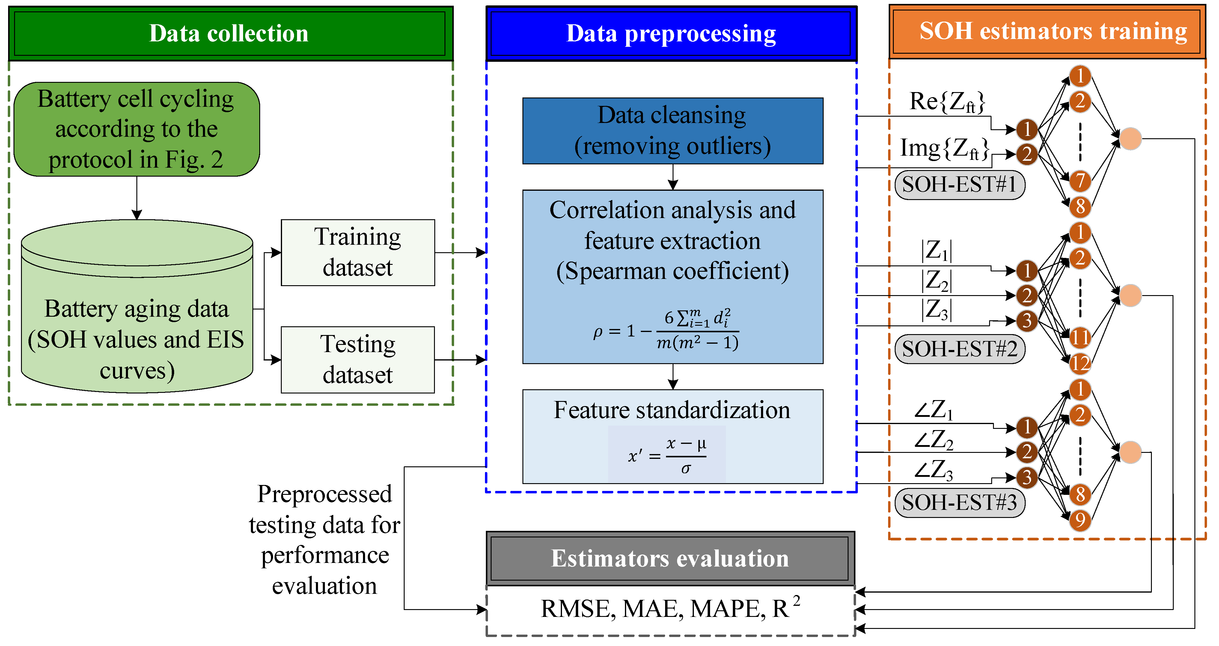
(1)

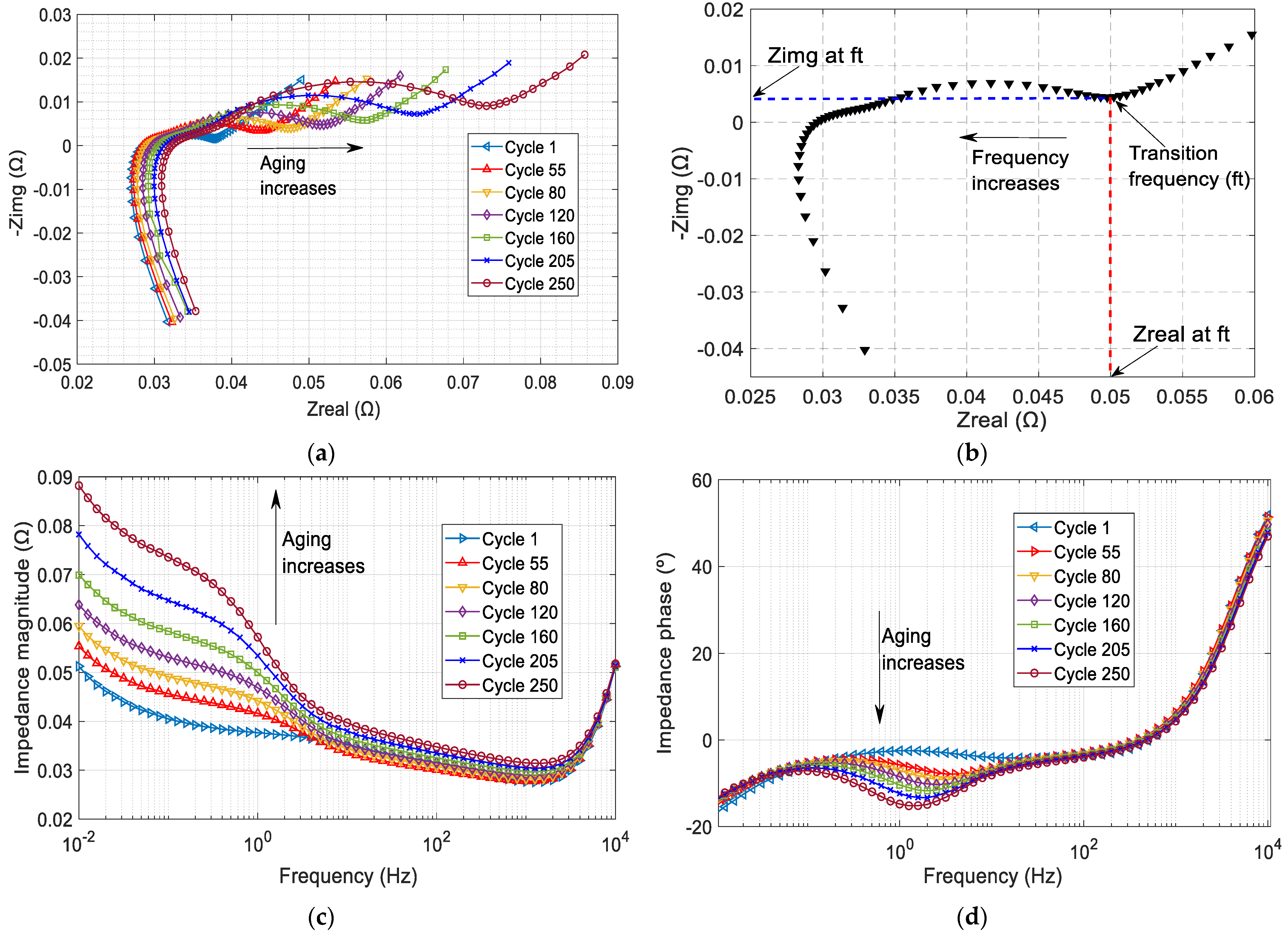
SOH_EST#1: This SOH estimator utilizes two indicators obtained from the complex impedance Nyquist plot. The two indicators are the impedance real part Re {Z_ft} and the impedance imaginary part Img {Z_ft} at the transition frequency f_t. The transition frequency is the frequency at which the Nyquist plot moves from the diffusion region to the charge transfer region in the low-frequency range. Figure 4a shows sample Nyquist plots of BAT#1 at different aging cycles. As shown, as the battery ages (as the SOH value decreases), the Nyquist plot moves to the right (which means a larger Re {Z_ft}) and moves up (which means a larger Img {Z_ft}). A single Nyquist plot is shown in Figure 4b with the transition frequency f_t, Re {Z_ft}, and Img {Z_ft} marked on the figure.

(2)

SOH_EST#2 and SOH_EST#3: These estimators utilize certain impedance magnitude and phase values (respectively) within key frequency ranges in which the impedance magnitude and phase show strong correlations with the SOH value. From Figure 4c, it can be noticed that the impedance magnitude curves show a strong correlation with SOH values, especially in the low-frequency range. Therefore, impedance magnitude values at certain frequency points can be utilized for SOH_EST#2. Similarly, from Figure 4d, it can be noticed that the impedance phase curves at different aging levels show a strong correlation with the SOH values in the low-frequency range. This means that impedance phase values at certain frequency points can be utilized for SOH_EST#3.

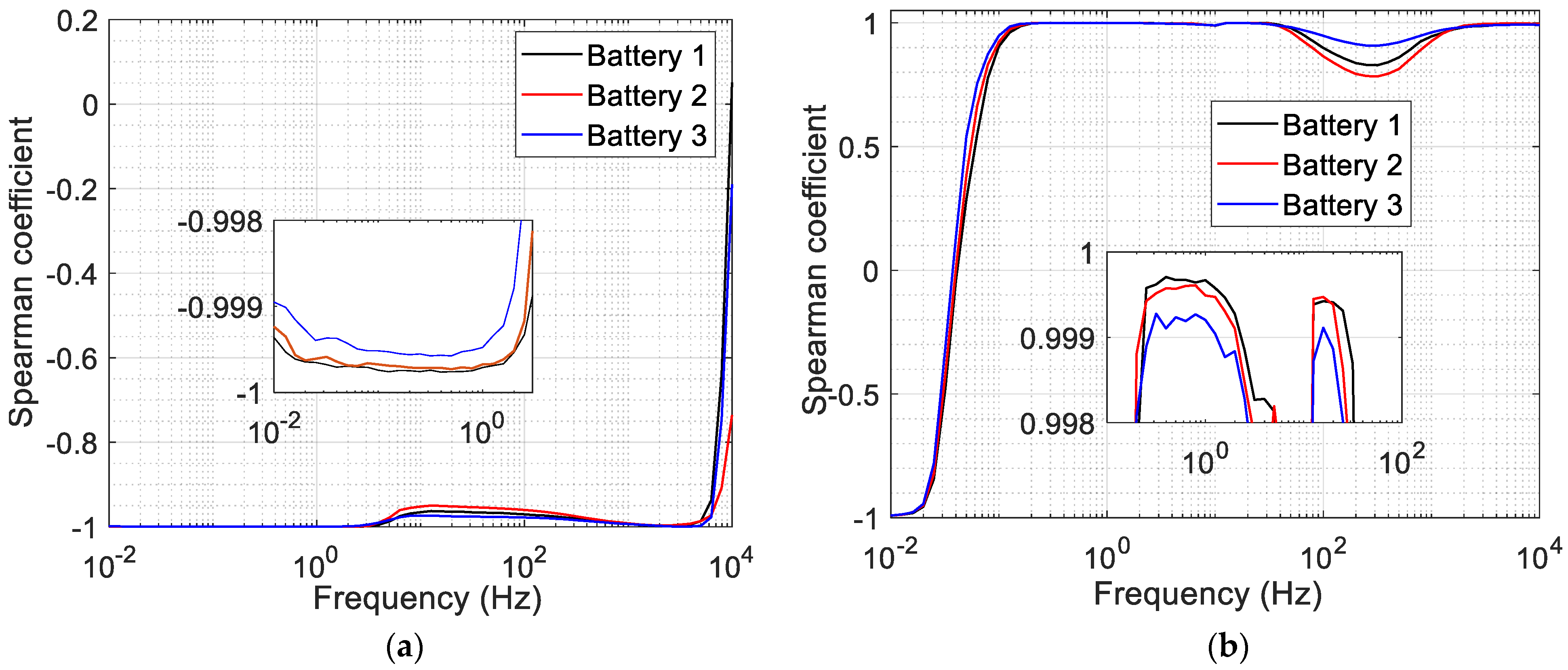
4. Correlation Analysis

To measure the degree to which the SOH value changes with different SOH indicators and to identify the indicators that exhibit a strong correlation with SOH values, a correlation analysis is performed. The Spearman correlation coefficient is selected to perform the correlation analysis. The Spearman correlation coefficient (ρ) evaluates the monotonic relationship between two variables and is expressed in (2) [50]:

$$\rho =1-{\displaystyle \frac{6\sum _{i=1}^m{d}_i^2}{m\left(m^2-1\right)}}$$

(2)

where d is the rank difference of each observation and m is the number of observations. To put this into the context of the battery aging data in this paper, the matrix Z_ft in (3) represents the transition frequency’s impedance real and imaginary values at m different SOH values. The matrix Z_ft has m rows (the number of SOH values obtained from battery aging) and two columns (one for Re {Z_ft} values and another for Img {Z_ft} values). The matrix |Z| in (4) represents the impedance magnitude values over a frequency range of 0.01 Hz to 10 kHz at m different SOH values. The matrix |Z| has m rows (the number of SOH values obtained from battery aging) and 61 columns (the number of impedance spectrum frequency points from 0.01 Hz to 10 kHz with 10 points per decade). Similarly, the matrix ∠Z in (5) represents the impedance phase values over a frequency range of 0.01 Hz to 10 kHz at m different SOH values. The goal is to study the relationship between the values in each column of the matrices (3)–(5) and the SOH values. For example, to study the relationship between Re {Z_ft} and the SOH value. This means studying the relationship between the first column in the Z_ft matrix expressed in (3) (Re {Z_ft1}, Re {Z_ft2}, Re {Z_ft3} … Re {Z_ftm}) and the SOH values vector (SOH₁, SOH₂, SOH₃ … SOH_m) that is expressed in (6), which includes the SOH values obtained during aging after each cycle. The same procedure is applied for the matrices |Z| and ∠Z. For example, studying the relationship between the impedance magnitudes at 0.01 Hz and the SOH value. This means studying the relationship between the first column in the |Z| matrix (|Z|_{1,0.01 Hz}, |Z|_{2,0.01 Hz}, |Z|_{3,0.01 Hz} … |Z|_{m,0.01 Hz}) and the SOH vector in (SOH₁, SOH₂, SOH₃ … SOH_m):

$${\mathrm{Z}}_{\mathrm{f}\mathrm{t}}=\left[\begin{array}{cc}{\mathrm{R}\mathrm{e}\{\mathrm{Z}}_{\mathrm{f}\mathrm{t}1}\}& {\mathrm{I}\mathrm{m}\mathrm{g}\{\mathrm{Z}}_{\mathrm{f}\mathrm{t}1}\}\\ {\mathrm{R}\mathrm{e}\{\mathrm{Z}}_{\mathrm{f}\mathrm{t}2}\}& {\mathrm{I}\mathrm{m}\mathrm{g}\{\mathrm{Z}}_{\mathrm{f}\mathrm{t}2}\}\\ ⋮& ⋮\\ {\mathrm{R}\mathrm{e}\{\mathrm{Z}}_{\mathrm{f}\mathrm{t}\mathrm{m}}\}& {\mathrm{I}\mathrm{m}\mathrm{g}\{\mathrm{Z}}_{\mathrm{f}\mathrm{t}\mathrm{m}}\}\end{array}\right]$$

(3)

$$\left|\mathrm{Z}\right|=\left[\begin{array}{ccc}{\left|\mathrm{Z}\right|}_{\mathrm{1,0.01}\mathrm{H}\mathrm{z}}& \cdots & {\left|\mathrm{Z}\right|}_{1,10\mathrm{k}\mathrm{H}\mathrm{z}}\\ {\left|\mathrm{Z}\right|}_{\mathrm{2,0.01}\mathrm{H}\mathrm{z}}& \cdots & {\left|\mathrm{Z}\right|}_{2,10\mathrm{k}\mathrm{H}\mathrm{z}}\\ ⋮& ⋮& ⋮\\ {\left|\mathrm{Z}\right|}_{m,0.01\mathrm{H}\mathrm{z}}& \cdots & {\left|\mathrm{Z}\right|}_{m,10\mathrm{k}\mathrm{H}\mathrm{z}}\end{array}\right]$$

(4)

$$\angle \mathrm{Z}=\left[\begin{array}{ccc}{\angle \mathrm{Z}}_{\mathrm{1,0.01}\mathrm{H}\mathrm{z}}& \cdots & {\angle \mathrm{Z}}_{1,10\mathrm{k}\mathrm{H}\mathrm{z}}\\ {\angle \mathrm{Z}}_{\mathrm{2,0.01}\mathrm{H}\mathrm{z}}& \cdots & {\angle \mathrm{Z}}_{2,10\mathrm{k}\mathrm{H}\mathrm{z}}\\ ⋮& ⋮& ⋮\\ {\angle \mathrm{Z}}_{m,0.01\mathrm{H}\mathrm{z}}& \cdots & {\angle \mathrm{Z}}_{m,10\mathrm{k}\mathrm{H}\mathrm{z}}\end{array}\right]$$

(5)

$$\mathrm{S}\mathrm{O}\mathrm{H}=\left[\begin{array}{c}{\mathrm{S}\mathrm{O}\mathrm{H}}_1\\ {\mathrm{S}\mathrm{O}\mathrm{H}}_2\\ ⋮\\ {\mathrm{S}\mathrm{O}\mathrm{H}}_m\end{array}\right]$$

(6)

To find the rank difference d of each observation, the values in each column in Z_ft, |Z|, and ∠Z are sorted in ascending order. Also, the SOH values in the SOH vector are sorted in ascending order. Then, the rank difference is calculated by finding the difference in each value’s rank and the rank of its corresponding SOH value. For example, the values of Re {Z_ft} [first column in (3)] are sorted in ascending order. Then, the rank difference d is calculated by finding the difference between the rank of each Re {Z_ft} value and the rank of its corresponding SOH value. The same procedure is applied to the second column in (3), which includes the values for Img {Z_ft}. Also, the same procedure is applied to every column in the impedance magnitude matrix in (4) and to every column in the impedance phase matrix in (5). In other words, the correlation coefficient is calculated between the SOH vector in (6) and every single column in (3)–(5). The Spearman correlation coefficient can take values between -1 (a perfect negative monotonic association) to +1 (a perfect positive monotonic association). The Spearman correlation coefficient is calculated for the Re {Z_ft} and Img {Z_ft} values at the transition frequency; the impedance magnitude value at every frequency point; and the impedance phase value at every frequency point. The Spearman correlation coefficients for Re {Z_ft} and Img {Z_ft} are summarized in

Table 2. Spearman correlation coefficients for Re {Z_ft} and Img {Z_ft}.

	Re {Zft}	Img {Zft}
Battery#1	−0.9996	−0.9997
Battery#2	−0.9995	−0.9996
Battery#3	−0.9993	−0.9993

. Both the Re {Z_ft} and Img {Z_ft} impedance values at the transition frequency show strong correlations with the SOH and thus can be used as input features for SOH_EST#1. Based on the aging data used in this paper, the transition frequency ranges from 1.585 Hz to 0.079 Hz at an SOH of ~96% and ~60%, respectively.

The Spearman correlation coefficients for the impedance magnitude values and impedance phase values are shown in Figure 5. From Figure 5a, it can be noticed that the impedance magnitude values at the lower frequency range of 0.01 Hz to 2 Hz show strong correlations with the SOH values, as shown in the zoomed-in view in Figure 5a. This means that impedance magnitude values within this frequency range are suitable SOH features for SOH_EST#2 (which utilizes impedance magnitude values at specific frequency points/ranges). From Figure 5b, the impedance phase values show strong correlations with the SOH values within two frequency ranges, one around 1 Hz and another between 10 Hz and 20 Hz, as shown in the zoomed-in view in Figure 5b. This means that impedance phase values within these two frequency ranges can be used as input features for SOH_EST#3 (which utilizes impedance phase values at specific frequency points/ranges).

5. ANN-Based SOH Estimation

The three SOH estimators explained in Section 3 are implemented using an artificial neural network (ANN). For SOH_EST#1, there are two input features that are Re {Z_ft} and Img {Z_ft} values at the transition frequency obtained from the impedance Nyquist plot. For SOH_EST#2, although many low-frequency points can be used as input features for the estimator based on the correlation analysis in the previous section, only the frequency points at which the impedance magnitude has the three largest absolute correlation coefficients are chosen as input features. This is to simplify the estimation model and to reduce its computational burden. Following the same intuition for SOH_EST#3, the impedance phase values of the three strongest correlations with SOH value are utilized to train and test SOH_EST#3.

Because the input features have different scales, the input data should be standardized, which can be applied as in (7):

$$x^{\prime }={\displaystyle \frac{x-\mathrm{\mu }}{\sigma }}$$

(7)

where x′ represents the standardized data point, x is the original data point, µ is the input data mean, and σ is the input data standard deviation.

After normalizing the input features, the training dataset is split into k-fold cross-validation sets. The k-fold cross-validation [51] is utilized to guide the SOH estimation models’ training and can be utilized as follows: for each fold of the training dataset, the model is trained on a part of the fold data points and tested/validated on the remainder of the fold data points. This process is repeated k times (i.e., k folds). For every fold, the validation error (the mean square error or “MSE”) is recorded, and if the average validation error of all training sessions is less than a pre-specified threshold, then the training process is considered complete, and the model becomes ready to be tested on the testing dataset that the model has never seen before. If the average validation error is not below the pre-specified threshold, the neural network hyperparameters need to be changed (e.g., changing the number of neurons in the hidden layer) until the average validation error becomes smaller than the pre-specified threshold. In this paper, the threshold for the average validation error is set to be 125 Coulombs (C), which is equivalent to ~0.035 Ah (125 C × 1 h/3600 s). This is equivalent to an SOH estimation error of 1.0% (0.035 Ah/3.5 Ah = 1.0%). The training dataset for each estimator is split into 10 folds (k = 10). Based on the k-fold cross-validation analysis, a three-layer ANN is utilized (input layer, hidden layer, and output layer) for the three SOH estimators. SOH_EST#1 utilizes an input layer of two neurons (SOH_EST#1 utilizes two features that are Re {Z_ft} and Img {Z_ft}) and a hidden layer of eight neurons. SOH_EST#2 utilizes an input layer of three neurons (SOH_EST#2 utilizes three impedance magnitude values) and a hidden layer of twelve neurons. SOH_EST#3 utilizes an input layer of three neurons (SOH_EST#3 utilizes three impedance phase values) and a hidden layer of nine neurons. For all SOH estimators in this paper, one neuron is utilized in the output layer to give the estimated SOH value.

The overall framework for the SOH estimators SOH_EST#1, SOH_EST#2, and SOH_EST#3 is shown in Figure 6. Before feeding the SOH features into the neural network, the input features go through a preprocessing stage. Data preprocessing includes data cleansing (removing any outliers that might exist), feature extraction using correlation analysis, and standardization [expressed in (7)].

The SOH estimators are trained, validated, and evaluated as follows: aging data (EIS curves and SOH values) for two batteries is used for SOH estimator training, and the estimator performance is evaluated using the aging data of the remaining battery (the SOH estimator performance is evaluated on a dataset that was not included in training). For example, aging data for BAT#1 and BAT#2 are used to train and validate the SOH estimator, where the SOH estimator’s performance is evaluated using the aging data of BAT#3. This way, there are multiple variations in the SOH estimator training and testing datasets. These variations are summarized in

Table 3. SOH estimator training, validation, and evaluation datasets summary.

SOH Estimator	SOH Estimation Model Designator	Training and Validation Data (Battery Numbers)	Performance Evaluation Data (Battery Number)	Frequency Points of Largest Correlation Coefficients
SOHEST#1	SOHEST#1_12_3	1, 2	3	Transition frequency ranges between 1.585 Hz and 0.079 Hz
	SOHEST#1_13_2	1, 3	2
	SOHEST#1_23_1	2, 3	1
SOHEST#2	SOHEST#2_12_3	1, 2	3	0.079 Hz, 0.158 Hz, 0.2 Hz
	SOHEST#2_13_2	1, 3	2	0.316 Hz, 0.398 Hz, 0.501 Hz
	SOHEST#2_23_1	2, 3	1	1.259 Hz, 1.585 Hz, 1.995 Hz
SOHEST#3	SOHEST#3_12_3	1, 2	3	12.59 Hz, 15.85 Hz, 19.95 Hz 12.59 Hz, 15.85 Hz, 19.95 Hz 12.59 Hz, 15.85 Hz, 19.95 Hz
	SOHEST#3_13_2	1, 3	2
	SOHEST#3_23_1	2, 3	1

. For example, SOH_{EST#1_12_3} represents the case in which SOH_EST#1 is trained using the aging data of BAT#1 and BAT#2 (i.e., “12” in the subscript of SOH_{EST#1_12_3}) where the performance of the SOH estimator is evaluated on the aging data of BAT#3 (i.e., “3” in the subscript of SOH_{EST#1_12_3}).

It should be mentioned that for SOH_EST#2, the frequency points of the correlation between the impedance magnitude and the SOH are not necessarily the same among all batteries. For example, for SOH_{EST#2_12_3}, the correlation analysis is performed on the data of BAT#1 and BAT#2 to identify the three frequency points at which the correlations between the impedance magnitude and the SOH are the largest. This analysis resulted in identifying 0.079 Hz, 0.158 Hz, and 0.2 Hz as the three frequency points of interest. However, this is different from those of SOH_{EST#2_23_1} and SOH_{EST#1_13_2}. The frequency points of interest for each estimator are summarized in Table 3 based on the correlation analysis of each training dataset. It should be mentioned that some of the frequency points at which the real and imaginary parts at the transition frequency are utilized for SOH_EST#1 might be the same frequency points at which the SOH_EST#2 features are extracted based on the correlation analysis, as shown in Table 3. However, this paper presents each of the SOH estimators separately and compares them.

The mean square error (MSE) is used as a loss function in the ANN training as expressed in (8), where y(i) is the value of the actual SOH in the training dataset and y′(i) is the value of the estimated SOH for the ith training sample:

$$MSE={\displaystyle \frac{1}{n}}{\sum }_{i=1}^n\left|y\left(i\right)-y\prime \left(i\right)\right|$$

(8)

To evaluate the estimation accuracy of the SOH estimators, the root mean square error (RMSE), the mean absolute error (MAE), the mean absolute percentage error (MAPE), and the coefficient of determination (R²) are utilized. These four indices are expressed in (9)–(12), where n is the number of outputs (the SOH values), A(i) is the actual output (the true SOH value), and P(i) is the estimated output (the estimated SOH value):

$$RMSE=\sqrt{{\displaystyle \frac{1}{n}}{\sum }_{i=1}^n{\left(A\left(i\right)-P\left(i\right)\right)}^2}$$

(9)

$$MAE={\displaystyle \frac{1}{n}}{\sum }_{i=1}^n\left|A\left(i\right)-P\left(i\right)\right|$$

(10)

$$MAPE={\displaystyle \frac{100}{n}}{\sum }_{i=1}^n{\displaystyle \frac{\left|A\left(i\right)-P\left(i\right)\right|}{A\left(i\right)}}$$

(11)

$$R^2=1-{\displaystyle \frac{{SS}_{res}}{{SS}_{tot}}}=1-{\displaystyle \frac{\sum _{i=1}^n{\left(A\left(i\right)-P\left(i\right)\right)}^2}{\sum _{i=1}^n{\left(A\left(i\right)-\overline{A\left(i\right)}\right)}^2}}$$

(12)

In (12), the term SS_res represents the total sum of squared residuals between the actual SOH values and the predicted SOH values. The term SS_tot represents the total sum of squares, i.e., the sum of squared differences between the actual SOH values and their mean value $\overline{A\left(i\right)}$.

Following the ANN model training details in this section, the SOH estimators’ performance indicators are summarized in

Table 4. SOH estimators’ performance results.

SOH Estimator	SOH Estimation Model Designator	RMSE (%)	MAE (%)	MAPE (%)	R2
SOHEST#1	SOHEST#1_12_3	1.76	1.30	1.94	0.978
	SOHEST#1_13_2	1.24	1.08	1.39	0.986
	SOHEST#1_23_1	0.67	0.54	0.68	0.995
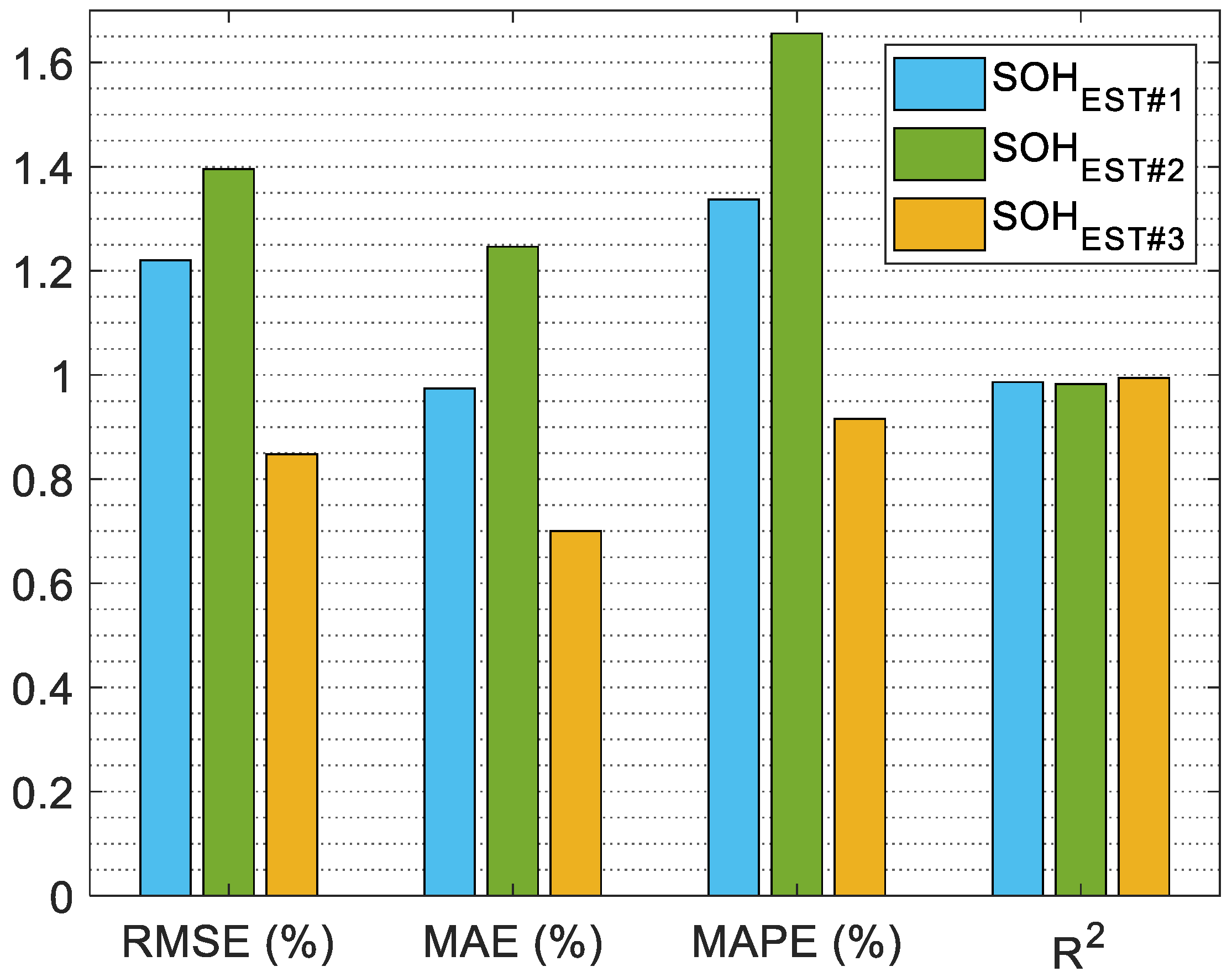
	Average	1.22	0.97	1.34	0.986
SOHEST#2	SOHEST#2_12_3	1.18	0.98	1.34	0.990
	SOHEST#2_13_2	1.40	1.29	1.66	0.986
	SOHEST#2_23_1	1.60	1.47	1.94	0.973
	Average	1.39	1.25	1.55	0.983
SOHEST#3	SOHEST#3_12_3	0.98	0.81	0.76	0.993
	SOHEST#3_13_2	0.74	0.60	0.90	0.996
	SOHEST#3_23_1	0.82	0.69	0.98	0.993
	Average	0.85	0.70	0.88	0.994

. Also, in Figure 7, the true SOH values versus the estimated SOH values are plotted, where the black dashed line represents the ideal estimation case (i.e., as if the estimated SOH value is equal to the actual SOH value).

From Table 4 and Figure 7, it is clear that all SOH estimators are capable of accurately estimating the SOH values based on their input features. The estimated SOH values match well with the actual SOH values. Table 4 also includes the average values of the RMSE, MAE, MAPE, and R² to make a comparison between the three estimators easier. The average values for all performance indicators are used to compare the three SOH estimators against each other, as shown in Figure 8. It can be noticed that SOH_EST#3 (which utilizes the impedance phase values at specific frequency points) shows the best performance among the three estimators; it has the lowest RMSE, MAE, and MAPE, in addition to the highest R². The second-best estimator is SOH_EST#1 (which utilizes the real and imaginary parts of the impedance at the transition frequency).

While multiple SOH estimators are presented in this paper, it is not necessary to use all of them. One estimator should be enough to predict the SOH value. Also, based on the analysis presented in this paper, it is not necessary to measure the entire EIS spectrum for any of the estimators. For SOH_EST#1, it would be only required to obtain the EIS data over a specific frequency range (between 1.585 Hz and 0.079 Hz). For SOH_EST#2 and SOH_EST#3, it would be only required to obtain the impedance magnitude and phase values at the frequency points that show the strongest correlations with SOH values. For instance, obtaining the impedance phase at 12.59 Hz, 15.85 Hz, and 19.95 Hz for SOH_EST#3. Another issue to be taken into consideration is the time taken to perform the EIS measurement. For example, obtaining the impedance magnitude/phase at a very low frequency (e.g., 0.02 Hz) takes more time than obtaining the EIS measurement at 20 Hz. This gives SOH_EST#3 an advantage over SOH_EST#2 and SOH_EST#1 in terms of speed since SOH_EST#3 utilizes impedance phase values at 12.59 Hz, 15.85 Hz, and 19.95 Hz (which takes ~6 s to measure), which are at a higher frequency range (i.e., a faster EIS measurement) compared with SOH_EST#2 (between 0.079 Hz and 0.2 Hz, which takes ~48 s to measure) and SOH_EST#1 (which requires measuring the EIS between 1.585 Hz and 0.079 Hz and that takes ~2 min). For all the estimators, the time taken to perform the EIS measurement is still significantly lower (a maximum of ~2 min) than the time needed to measure the entire EIS curve (~17 min), which is equivalent to an ~88% reduction in measurement time.

6. Conclusions

This paper presented three EIS-based SOH estimators for lithium-ion batteries by utilizing different features obtained from the impedance Nyquist plot, impedance magnitude curve, and impedance phase curve. This article (a) presented new health features obtained from the Nyquist plot for SOH estimation, (b) presented a correlation-analysis-based framework to obtain impedance magnitude and impedance phase values to be utilized for SOH estimation, and (c) presented and evaluated ANN-based SOH estimators. The performance evaluation of the three developed SOH estimators shows that all estimators are capable of accurately predicting the SOH values with minor/negligible differences in their accuracies.

Future work includes, but is not limited to, testing the presented SOH estimators on larger battery aging datasets of high degradation levels, in addition to comparing the presented estimation methods with other methods in the literature, such as Kalman filter and particle filter-based methods. Also, different types of batteries can be considered (different brands and different capacities) to enhance the generalizability of SOH estimation models/techniques.

References

- Manzetti, S.; Mariasiu, F. Electric vehicle battery technologies: From present state to future systems. Renew. Sustain. Energy Rev. 2015, 51, 1004–1012. [Google Scholar] [CrossRef]
- Deng, Z.; Hu, X.; Li, P.; Lin, X.; Bian, X. Data-Driven Battery State of Health Estimation Based on Random Partial Charging Data. IEEE Trans. Power Electron. 2022, 37, 5021–5031. [Google Scholar] [CrossRef]
- Xia, Z.; Qahouq, J.A.A. Lithium-ion battery ageing behavior pattern characterization and state-of-health estimation using data-driven method. IEEE Access 2021, 9, 98287–98304. [Google Scholar]
- Lee, J.; Kwon, D.; Pecht, M.G. Reduction of li-ion battery qualification time based on prognostics and health management. IEEE Trans. Ind. Electron. 2018, 66, 7310–7315. [Google Scholar]
- Soyoye, B.D.; Bhattacharya, I.; Anthony Dhason, M.V.; Banik, T. State of Charge and State of Health Estimation in Electric Vehicles: Challenges, Approaches and Future Directions. Batteries 2025, 11, 32. [Google Scholar] [CrossRef]
- Nuroldayeva, G.; Serik, Y.; Adair, D.; Uzakbaiuly, B.; Bakenov, Z. State of Health Estimation Methods for Lithium-Ion Batteries. Int. J. Energy Res. 2023, 2023, 4297545. [Google Scholar]
- Akram, M.N.; Abdul-Kader, W. Repurposing Second-Life EV Batteries to Advance Sustainable Development: A Comprehensive Review. Batteries 2024, 10, 452. [Google Scholar] [CrossRef]
- Zhao, Y.; Qahouq, J.A.A. Second-Use Battery System for EV Charging Stations. In Proceedings of the 2023 IEEE Energy Conversion Congress and Exposition (ECCE), Nashville, TN, USA, 29 October–2 November 2023; pp. 2122–2126. [Google Scholar]
- Vignesh, S.; Che, H.S.; Selvaraj, J.; Tey, K.S.; Lee, J.W.; Shareef, H.; Errouissi, R. State of Health (SoH) estimation methods for second life lithium-ion battery—Review and challenges. Appl. Energy 2024, 369, 123542. [Google Scholar]
- Vermeer, W.; Mouli, G.R.C.; Bauer, P. A comprehensive review on the characteristics and modeling of lithium-ion battery aging. IEEE Trans. Transp. Electrif. 2021, 8, 2205–2232. [Google Scholar]
- Han, X.; Lu, L.; Zheng, Y.; Feng, X.; Li, Z.; Li, J.; Ouyang, M. A review on the key issues of the lithium ion battery degradation among the whole life cycle. ETransportation 2019, 1, 100005. [Google Scholar]
- Kumar, R.R.; Bharatiraja, C.; Udhayakumar, K.; Devakirubakaran, S.; Sekar, K.S.; Mihet-Popa, L. Advances in Batteries, Battery Modeling, Battery Management System, Battery Thermal Management, SOC, SOH, and Charge/Discharge Characteristics in EV Applications. IEEE Access 2023, 11, 105761–105809. [Google Scholar] [CrossRef]
- Ahwiadi, M.; Wang, W. Battery Health Monitoring and Remaining Useful Life Prediction Techniques: A Review of Technologies. Batteries 2025, 11, 31. [Google Scholar] [CrossRef]
- Yang, B.; Qian, Y.; Li, Q.; Chen, Q.; Wu, J.; Luo, E.; Xie, R.; Zheng, R.; Yan, Y.; Su, S. Critical summary and perspectives on state-of-health of lithium-ion battery. Renew. Sustain. Energy Rev. 2024, 190, 114077. [Google Scholar]
- Demirci, O.; Taskin, S.; Schaltz, E.; Demirci, B.A. Review of battery state estimation methods for electric vehicles-Part II: SOH estimation. J. Energy Storage 2024, 96, 112703. [Google Scholar]
- Yao, L.; Xu, S.; Tang, A.; Zhou, F.; Hou, J.; Xiao, Y.; Fu, Z. A review of lithium-ion battery state of health estimation and prediction methods. World Electr. Veh. J. 2021, 12, 113. [Google Scholar] [CrossRef]
- Yang, S.; Zhang, C.; Jiang, J.; Zhang, W.; Zhang, L.; Wang, Y. Review on state-of-health of lithium-ion batteries: Characterizations, estimations and applications. J. Clean. Prod. 2021, 314, 128015. [Google Scholar]
- Guha, A.; Patra, A. State of health estimation of lithium-ion batteries using capacity fade and internal resistance growth models. IEEE Trans. Transp. Electrif. 2017, 4, 135–146. [Google Scholar]
- Zhang, C.; Liu, J.; Sharkh, S. Identification of dynamic model parameters for lithium-ion batteries used in hybrid electric vehicles. In Proceedings of the International Symposium on Electric Vehicles (ISEV), Beijing, China, 1 September 2009. [Google Scholar]
- Bao, Y.; Dong, W.; Wang, D. Online Internal Resistance Measurement Application in Lithium Ion Battery Capacity and State of Charge Estimation. Energies 2018, 11, 1073. [Google Scholar] [CrossRef]
- Fu, Y.; Xu, J.; Shi, M.; Mei, X. A fast impedance calculation-based battery state-of-health estimation method. IEEE Trans. Ind. Electron. 2021, 69, 7019–7028. [Google Scholar]
- Wang, D.; Bao, Y.; Shi, J. Online lithium-ion battery internal resistance measurement application in state-of-charge estimation using the extended Kalman filter. Energies 2017, 10, 1284. [Google Scholar] [CrossRef]
- Movassagh, K.; Raihan, A.; Balasingam, B.; Pattipati, K. A Critical Look at Coulomb Counting Approach for State of Charge Estimation in Batteries. Energies 2021, 14, 4074. [Google Scholar] [CrossRef]
- Schaltz, E.; Stroe, D.-I.; Nørregaard, K.; Ingvardsen, L.S.; Christensen, A. Incremental capacity analysis applied on electric vehicles for battery state-of-health estimation. IEEE Trans. Ind. Appl. 2021, 57, 1810–1817. [Google Scholar] [CrossRef]
- Xia, F.; Wang, K.; Chen, J. State of health and remaining useful life prediction of lithium-ion batteries based on a disturbance-free incremental capacity and differential voltage analysis method. J. Energy Storage 2023, 64, 107161. [Google Scholar] [CrossRef]
- Huang, Z.; Best, M.; Knowles, J.; Fly, A. Adaptive Piecewise Equivalent Circuit Model With SOC/SOH Estimation Based on Extended Kalman Filter. IEEE Trans. Energy Convers. 2023, 38, 959–970. [Google Scholar] [CrossRef]
- Andre, D.; Appel, C.; Soczka-Guth, T.; Sauer, D.U. Advanced mathematical methods of SOC and SOH estimation for lithium-ion batteries. J. Power Sources 2013, 224, 20–27. [Google Scholar] [CrossRef]
- Fang, F.; Ma, C.; Ji, Y. A Method for State of Charge and State of Health Estimation of Lithium Batteries Based on an Adaptive Weighting Unscented Kalman Filter. Energies 2024, 17, 2145. [Google Scholar] [CrossRef]
- Liu, D.; Yin, X.; Song, Y.; Liu, W.; Peng, Y. An On-Line State of Health Estimation of Lithium-Ion Battery Using Unscented Particle Filter. IEEE Access 2018, 6, 40990–41001. [Google Scholar] [CrossRef]
- Wu, T.; Liu, S.; Wang, Z.; Huang, Y. SOC and SOH joint estimation of lithium-ion battery based on improved particle filter algorithm. J. Electr. Eng. Technol. 2022, 17, 307–317. [Google Scholar] [CrossRef]
- Bi, J.; Zhang, T.; Yu, H.; Kang, Y. State-of-health estimation of lithium-ion battery packs in electric vehicles based on genetic resampling particle filter. Appl. Energy 2016, 182, 558–568. [Google Scholar] [CrossRef]
- Zhang, Z.; Zhang, R.; Liu, X.; Zhang, C.; Sun, G.; Zhou, Y.; Yang, Z.; Liu, X.; Chen, S.; Dong, X.; et al. Advanced State-of-Health Estimation for Lithium-Ion Batteries Using Multi-Feature Fusion and KAN-LSTM Hybrid Model. Batteries 2024, 10, 433. [Google Scholar] [CrossRef]
- Al-Smadi, M.K.; Qahouq, J.A.A. SOH Estimation Algorithm and Hardware Platform for Lithium-ion Batteries. In Proceedings of the 2024 IEEE Vehicle Power and Propulsion Conference (VPPC), Washington DC, USA, 7–10 October 2024; pp. 1–5. [Google Scholar]
- Abu Qahouq, J. An Electrochemical Impedance Spectrum-Based State of Health Differential Indicator with Reduced Sensitivity to Measurement Errors for Lithium–Ion Batteries. Batteries 2024, 10, 368. [Google Scholar] [CrossRef]
- Zhang, Y.; Tang, Q.; Zhang, Y.; Wang, J.; Stimming, U.; Lee, A.A. Identifying degradation patterns of lithium ion batteries from impedance spectroscopy using machine learning. Nat. Commun. 2020, 11, 1706. [Google Scholar] [PubMed]
- Xia, Z.; Qahouq, J.A.A. State of Health Estimation of Lithium-Ion Batteries Using Neuron Network and 1kHz Impedance Data. In Proceedings of the 2020 IEEE Energy Conversion Congress and Exposition (ECCE), Detroit, MI, USA; 2020; pp. 1968–1972. [Google Scholar]
- Love, C.T.; Dubarry, M.; Reshetenko, T.; Devie, A.; Spinner, N.; Swider-Lyons, K.E.; Rocheleau, R. Lithium-ion cell fault detection by single-point impedance diagnostic and degradation mechanism validation for series-wired batteries cycled at 0 C. Energies 2018, 11, 834. [Google Scholar] [CrossRef]
- Eddahech, A.; Briat, O.; Woirgard, E.; Vinassa, J.M. Remaining useful life prediction of lithium batteries in calendar ageing for automotive applications. Microelectron. Reliab. 2012, 52, 2438–2442. [Google Scholar] [CrossRef]
- Xia, Z.; Qahouq, J.A.A. State-of-charge balancing of lithium-ion batteries with state-of-health awareness capability. IEEE Trans. Ind. Appl. 2020, 57, 673–684. [Google Scholar] [CrossRef]
- Xia, Z.; Qahouq, J.A.A. Adaptive and Fast State of Health Estimation Method for Lithium-ion Batteries Using Online Complex Impedance and Artificial Neural Network. In Proceedings of the 2019 IEEE Applied Power Electronics Conference and Exposition (APEC), Anaheim, CA, USA, 17–21 March 2019; pp. 3361–3365. [Google Scholar]
- Li, C.; Yang, L.; Li, Q.; Zhang, Q.; Zhou, Z.; Meng, Y.; Zhao, X.; Wang, L.; Zhang, S.; Li, Y. SOH estimation method for lithium-ion batteries based on an improved equivalent circuit model via electrochemical impedance spectroscopy. J. Energy Storage 2024, 86, 111167. [Google Scholar]
- Xiong, R.; Tian, J.; Mu, H.; Wang, C. A systematic model-based degradation behavior recognition and health monitoring method for lithium-ion batteries. Appl. Energy 2017, 207, 372–383. [Google Scholar]
- Luo, F.; Huang, H.; Ni, L.; Li, T. Rapid prediction of the state of health of retired power batteries based on electrochemical impedance spectroscopy. J. Energy Storage 2021, 41, 102866. [Google Scholar]
- Wang, X.; Wei, X.; Dai, H. Estimation of state of health of lithium-ion batteries based on charge transfer resistance considering different temperature and state of charge. J. Energy Storage 2019, 21, 618–631. [Google Scholar]
- LGChem. Product Specification: Rechargeable Lithium Ion Battery, Model: INR18650 MJ1 3500mAh; LGChem: Seoul, Republic of Korea, 2024. [Google Scholar]
- Admiral Instruments, “Squidstat Cycler—Base Model”. Available online: https://www.admiralinstruments.com/_files/ugd/dc5bf5_c4286dd7c5be411c9ad415c452fe5c88.pdf (accessed on 13 March 2025).
- Westerhoff, U.; Kroker, T.; Kurbach, K.; Kurrat, M. Electrochemical impedance spectroscopy based estimation of the state of charge of lithium-ion batteries. J. Energy Storage 2016, 8, 244–256. [Google Scholar]
- Messing, M.; Shoa, T.; Habibi, S. Electrochemical impedance spectroscopy with practical rest-times for battery management applications. IEEE Access 2021, 9, 66989–66998. [Google Scholar] [CrossRef]
- Li, Q.; Yi, D.; Dang, G.; Zhao, H.; Lu, T.; Wang, Q.; Lai, C.; Xie, J. Electrochemical Impedance Spectrum (EIS) Variation of Lithium-Ion Batteries Due to Resting Times in the Charging Processes. World Electr. Veh. J. 2023, 14, 321. [Google Scholar] [CrossRef]
- Spearman, C. The Proof and Measurement of Association Between Two Things; Appleton-Century-Crofts: East Norwalk, CT, USA, 1961; pp. 45–58. [Google Scholar]
- Berrar, D. Cross-Validation. In Encyclopedia of Bioinformatics and Computational Biology; Ranganathan, S., Gribskov, M., Nakai, K., Schönbach, C., Eds.; Academic Press: Oxford, UK, 2019; pp. 542–545. [Google Scholar]