Article

A Smart Evolving Fuzzy Predictor with Customized Firefly Optimization for Battery RUL Prediction

by
Mohamed Ahwiadi
and
Wilson Wang
*
Department of Mechanical and Mechatronics Engineering, Lakehead University, Thunder Bay, ON P7B 5E1, Canada
*
Author to whom correspondence should be addressed.
Batteries 2025, 11(10), 362; https://doi.org/10.3390/batteries11100362
Submission received: 12 August 2025 / Revised: 23 September 2025 / Accepted: 29 September 2025 / Published: 30 September 2025

Abstract

Accurate prediction of system degradation and remaining useful life (RUL) is essential for reliable health monitoring of Lithium-ion (Li-ion) batteries, as well as other dynamic systems. While evolving systems can offer adequate adaptability to the nonstationary and nonlinear behavior of battery degradation, existing methods often face challenges such as uncontrolled rule growth, limited adaptability, and reduced accuracy under noisy conditions. To address these limitations, this paper presents a smart evolving fuzzy predictor with customized firefly optimization (SEFP-FO) to provide a better solution for battery RUL prediction. The proposed SEFP-FO technique introduces two main contributions: (1) An activation- and distance-aware penalization strategy is proposed to govern rule evolution by evaluating the structural relevance of incoming data. This mechanism can control rule growth while maintaining model convergence. (2) A customized firefly algorithm is suggested to optimize the antecedent parameters of newly generated fuzzy rules, thereby enhancing prediction accuracy and improving the predictor’s adaptive capability to time-varying system conditions. The effectiveness of the proposed SEFP-FO technique is first validated by simulation using nonlinear benchmark datasets, which is then applied to Li-ion battery RUL predictions.

Graphical Abstract

1. Introduction

Lithium-ion (Li-ion) batteries have become the backbone of energy storage and modern technological ecosystems. Their high energy density, lightweight design, and rechargeability make them the preferred power source across a wide range of applications such as electric vehicles, smartphones, medical devices, and grid-scale energy storage systems [1,2,3]. However, Li-ion batteries experience degradation over time. With each charge–discharge cycle, battery capacity decreases, internal resistance rises, and overall operational efficiency declines [4,5]. Eventually, this aging process reaches a critical point, known as the battery’s end-of-life, when it becomes inefficient, unreliable or even hazardous. The implications are especially serious in safety-critical applications such as electric vehicles, where unexpected battery failure can lead to service disruption, safety risks and significant financial losses [2,4,6].
In this context, accurate and timely prediction of a battery’s remaining useful life (RUL) has become a key pillar of modern battery management systems. Effective RUL estimation can enable proactive maintenance, enhance system reliability, and support informed planning and health management [7,8]. The practical importance of accurate RUL prediction has been highlighted across multiple domains. In electric vehicles, for example, studies such as [9] show that RUL-aware prediction strategies are essential for safe operation and energy efficiency. Beyond electric vehicles, recent reviews emphasize that RUL prediction is equally critical in other fields, such as grid-scale storage, where unexpected failures can disrupt power supply, and medical devices, where battery reliability is directly linked to patient safety [1,2,3,7,10]. Together, these examples make it clear that RUL prediction is not only a technical challenge but also a practical necessity for ensuring safety, sustainability, and cost-effectiveness in real applications. On the other hand, RUL prediction remains a highly challenging task, as battery degradation is influenced by a complex interplay of nonlinear and nonstationary processes that evolve under different operating conditions and usage patterns [11,12,13]. Factors such as temperature, load profiles, charge–discharge strategies, and intrinsic electrochemical characteristics make the underlying degradation behavior difficult to model accurately [5,10,14]. Furthermore, the presence of measurement noise and system-level uncertainties limits the effectiveness of traditional model-based and static data-driven methods [6,11].
Researchers have explored a wide range of modeling strategies for battery RUL prediction, which can be broadly categorized into model-based and data-driven approaches. Model-based techniques aim to replicate the internal behavior of Li-ion batteries through mathematical representations of battery physical, electrochemical, or electrical characteristics. These include physics-informed models that simulate electrochemical reactions [12,13] and equivalent circuit models that approximate battery dynamics using electrical components such as resistors, capacitors, and voltage sources [3,15]. Such models are commonly used to estimate key internal states, including capacity fade, internal resistance, and state of charge [7,16].
In practice, model-based methods are often integrated with state estimation algorithms to improve battery health monitoring and prediction accuracy. For example, the extended Kalman filter and the unscented Kalman filter, along with their improved variants, are widely applied for this purpose [5,6,17]. Reference [18] applies an extended Kalman filter with a Thevenin equivalent-circuit model to estimate the state of charge under a standard driving cycle. Although this method achieves good accuracy under moderate operating conditions, it shows increased errors when battery nonlinearities become more pronounced. To address these nonlinearities, the unscented Kalman filter has been applied in several studies [19,20], which could provide better performance in capturing system dynamics for battery state estimation.
Particle filters (PFs) are also employed to deal with nonlinearities and non-Gaussian noise [21]. For instance, Ref. [22] integrates a PF with an equivalent circuit model to predict battery capacity fade and resistance growth for RUL prediction under variable loading conditions. Similarly, Ref. [23] uses resistance growth as a degradation indicator to improve long-term forecasting accuracy. Several advanced PF variants are also introduced in the literature to overcome the limitations of the classical PF, including a mutated PF [24], AI-driven PF [13], and artificial fish swarm algorithm-based PF [25].
Although these model-based methods are well-suited for scenarios where partial model knowledge is available, model-based approaches still face several limitations. Their performance is highly dependent on the accuracy of the underlying models, which are often difficult to construct due to complex electrochemical behaviors and variability across battery types [12,15,21]. Accurate parameter identification typically requires laborious offline experiments or expert knowledge [4,15]. In addition, model-based estimators are sensitive to measurement noise and often rely on simplified assumptions such as Gaussian distributions or static system dynamics, which may not hold under real-world, dynamic operating conditions [5,16].
To deal with these shortcomings, several hybrid frameworks are introduced that combine the physical interpretability of model-based estimation with the flexibility of machine learning techniques. For example, Ref. [26] integrates a nonlinear autoregressive model with a regularized PF, which allows the PF to leverage the predictive capability of the nonlinear autoregressive model during prognostic updates. Reference [27] presents a hybrid electrochemical–thermal model combined with an unscented Kalman filter to improve RUL prediction under dynamic operating conditions. In addition, Ref. [28] combines variational mode decomposition with a PF and Gaussian process regression to denoise degradation trends and enhance battery RUL forecasting accuracy. While such frameworks could improve accuracy and generalization, they also introduce implementation complexity, and their overall reliability still depends on the accuracy of each component in the framework [15]. These challenges can impact the accuracy and robustness of model-based prognostic frameworks in practical applications.
In contrast to model-based methods, data-driven approaches have gained significant traction in recent decades for battery RUL prediction and health management, due to their flexibility and reduced dependence on detailed physical or electrochemical models. These approaches analyze historical measurements of voltage, current, temperature, or capacity to recognize complex relationships between observable inputs and degradation states, without requiring knowledge of the internal battery mechanisms [29,30,31,32]. Early data-driven approaches employ classical machine learning techniques such as support vector regression, relevance vector machines, Gaussian process regression, and autoregression to track battery capacity fade and estimate the RUL from observable battery signals [33,34,35,36]. These techniques are relatively easy to implement and can perform well under stable or stationary operating conditions or for short-horizon predictions. However, they often have difficulties in being generalized across different aging mechanisms or under dynamic environments [34,37].
To address these limitations, deep learning techniques have been introduced as an alternative for Li-ion battery prognostics. These techniques can extract high-level and nonlinear features directly from raw time-series battery signals. Architectures such as convolutional neural networks, recurrent neural networks, long short-term memory networks, and gated recurrent units have shown notable efficiency in capturing temporal dependencies and identifying complex degradation trends in battery behavior [38,39,40,41]. For instance, convolutional neural networks are effective for extracting localized features from sequential data; recurrent neural networks, especially long short-term memory networks and gated recurrent units, are capable of modeling long-term dependencies in battery dynamic behavior [40,42]. These deep architectures have been adopted for battery state-of-health (SOH) estimation and RUL prediction [39,43].
Despite these advances, deep learning models often operate as “black boxes”, making them difficult to interpret and validate [44,45]. They also require large volumes of labeled degradation data for training, which may not always be available in applications, particularly across different degradation phases or failure modes. Furthermore, these deep models tend to suffer from overfitting and poor adaptability in online and/or nonstationary environments where battery behavior drifts over time [41,44,45].
In recent years, evolving fuzzy system (eFS) techniques have attracted increasing attention as an adaptive and powerful modeling approach for tackling the limitations of conventional data-driven methods. These techniques are well-suited for modeling complex, nonlinear, and time-varying systems. Unlike traditional data-driven methods that rely on fixed structures and require offline training to cope with changing conditions, eFS techniques offer a flexible architecture that can evolve both their structure and parameters in real time. This ability to adapt on the fly makes them especially appealing for applications involving streaming sensor data and nonstationary behavior, such as battery management systems [46,47,48]. These systems typically begin empty and gradually expand as new patterns appear in the data. This structure-learning capability allows eFS techniques to adapt continuously to changes in distribution or dynamics without the need for retraining from scratch [46,49]. Several mechanisms have been proposed for managing rule generation and adaptation in eFS techniques, including potential-based measures [50,51,52,53] and distance-based measures [54,55,56,57,58]. For example, the evolving Takagi–Sugeno (eTS) technique introduced in [50] uses a recursive potential measure derived from Cauchy-type functions to determine the uniqueness of incoming data points and trigger the generation of new rules. Similarly, the technique in [53] employs dynamically evolving clustering to monitor changes in local density and guide structure adaptation. Distance-based methods, such as those relying on Euclidean or Mahalanobis distances [54,58], assess geometric proximity between new data and existing rule centers to decide whether a new rule is required. Moreover, rule activation thresholds are used in [59,60,61] to measure the influence of new data on existing rules, where low activation across all rules signals the need for expansion.
Several studies demonstrate that eFS techniques are effective in different applications such as fault diagnosis, online forecasting, and intelligent control [52,53,55,57]. They usually outperform other static and fixed-structure models in dynamic environments. For example, [53] shows that evolving predictor achieves lower errors than feedforward neural networks, radial basis function networks, and an adaptive neuro-fuzzy inference system on the Mackey–Glass benchmark. Reference [54] further confirms that the evolving fuzzy method achieves better results than conventional batch-trained models in nonlinear dynamic system identification tasks. It is highlighted in [50] that fixed fuzzy models lack adaptability and often fail under changing conditions, whereas evolving fuzzy rule-based models can continuously adjust their structures online and achieve higher accuracy. In the context of battery prognostics, an adaptive eFS framework in [48] is compared with a static adaptive neuro-fuzzy inference system (16 rules) and a model-based particle filter, which demonstrates accurate and stable RUL predictions across horizons. Table 1 provides a comparative overview of these representative approaches in terms of accuracy, interpretability, adaptiveness, robustness to noise, and computational cost.
However, despite their promising effects, existing eFS techniques face significant challenges, especially for long-horizon prediction tasks under noisy and nonlinear conditions, such as those found in battery RUL prediction and SOH monitoring. One major limitation is rule overgrowth, where the number of fuzzy rules increases rapidly over time due to sensitivity to noise or overly aggressive detection of unfamiliar data patterns. The problem of rule overgrowth increases model complexity, reduces interpretability, and raises computational cost [48,62]. Many approaches also rely on fixed thresholds or heuristic criteria for rule evolution, which makes it hard for them to adapt to varying operating conditions. As noted in [50,63], static thresholds may lead to unnecessary rule evolution or trigger excessive rule generation in noisy settings. Another critical shortcoming is that the existing evaluation of input uniqueness, typically based on statistical deviation or geometric distance, cannot account for the current structural information, which can lead to underfitting and misaligned rule evolution under data drift [48,62,63].
These gaps highlight the need for a new prediction technology that can capture the dynamic behavior of Li-ion batteries and have adaptive capability to drifting operating conditions while maintaining a compact structure and good accuracy under noisy and nonlinear conditions. Although eFS techniques can overcome the fixed-structure limitations, they still require enhancements to regulate rule growth for processing accuracy. Guided by this motivation, this work presents a novel smart evolving fuzzy predictor with customized firefly optimization (SEFP-FO) for battery RUL prediction. The aim is to improve the reliability and scalability of long-horizon predictions in battery SOH monitoring and RUL estimation. The SEFP-FO architecture is designed to retain the reasoning transparency of conventional eFS models while addressing their key limitations through a unified enhancement mechanism.
The proposed SEFP-FO technique introduces two key contributions: (1) An activation- and distance-aware penalization (ADAP) strategy is suggested to enhance the evaluation of input distinctiveness. This is achieved by integrating structural knowledge of the existing rule base and rule evolution mechanism, in order to determine whether a new rule should be generated. (2) A customized firefly algorithm (CFA) is proposed to optimize the antecedent parameters of newly generated rules to improve system performance. Unlike the standard firefly algorithm (FA), the CFA introduces an adaptive attractiveness mechanism to guide the search and exploration.
This study is guided by the following research questions: (1) Can SEFP-FO achieve higher prediction accuracy with a compact rule base compared to existing evolving fuzzy systems? (2) Can the ADAP strategy effectively control rule growth without harming accuracy? (3) Can integrating the ADAP and CFA mechanisms enhance rule evolution and robustness under noisy and nonlinear conditions?
The remainder of this paper is organized as follows: Section 2 presents the proposed SEFP-FO technique, including its evolving fuzzy rule structure, the ADAP strategy, and the customized firefly optimization. The effectiveness of the SEFP-FO is evaluated in Section 3 through simulation studies and Li-ion battery RUL prediction. Some concluding remarks and future work are summarized in Section 4.

2. The Proposed SEFP-FO Technique

This section discusses the proposed SEFP-FO technique. It is designed to overcome limitations in traditional eFS methods in rule explosion and accuracy degradation during long-term prediction. The proposed SEFP-FO technique includes two innovations: an ADAP mechanism to regulate rule creation and CFA to fine-tune the antecedent parameters of newly generated fuzzy rules. The proposed SEFP-FO technique operates within first-order Takagi-Sugeno (TS-1) fuzzy scheme and dynamically updates its rule base with continuous adaptation to streaming data.

2.1. Evolving Fuzzy Rule Structure

The proposed SEFP-FO technique introduces an evolving fuzzy inference system designed for multi-steps-ahead time series prediction. It is built on a TS-1 scheme [48], where each fuzzy rule maps a set of inputs to a designated output. As new data streams in, the system incrementally generates and/or adapts fuzzy rules to capture characteristic patterns in the input-output space. For each prediction step s, the model constructs localized rules based on n input values observed at time step k, so as to estimate the target output associated with that step.
Each fuzzy rule R j represents a local model formed using a set of antecedent propositions and consequent operations. Fuzzy rule R j with n input variables can be defined as:
Rule j: If ( y k is A 1 j ) and ( y k s is A 2 j ) and ( y k 2 s is A 3 j ) and…, and ( y k ( n 1 ) s is A i j )
Then   y ^ k + s = θ 0 j + i = 1 n θ i j y k ( i 1 ) s
where j [ 1 , N ] denotes the j-th fuzzy rule; N is the total number of rules; A i j denote the fuzzy sets associated with the i-th input in the rule j; and { θ 0 j , θ 1 j , , θ n j } are the consequent linear parameters.
To facilitate partitioning of the input/output spaces, all fuzzy sets utilize Gaussian membership functions (MFs) due to their smooth behavior and unique analytical properties [64]. The MF grade (i.e., premise parameter) represents the degree of activation of the fuzzy sets A i j for the i-th input at the time step k, computed as:
μ A i j ( y k ( i 1 ) s ) = exp ( y k ( i 1 ) s c i j ) 2 2 σ i j 2
where c i j and σ i j are the respective center and width of the Gaussian MF for the i-th input in rule j, which are the premise nonlinear parameters. For simplicity, they will be referred to as c j and σ j in the remainder of this paper.
The rule firing strength at time k, denoted by w j ( k ) , quantifies its relative strength and represents the joint activation of all inputs. If a T-norm operator is applied, the rule firing strength can be calculated as:
w j ( k ) = i = 1 n μ A i j ( y k + ( i 1 ) s )
To normalize the influence of each rule, the normalized firing strengths are scaled by:
w ¯ j ( k ) = w j ( k ) j = 1 N w j ( k )
The predicted output by the rule j is projected by applying the local consequent linear model to the input space:
y ^ j ( k + s ) = θ 0 j + i = 1 n θ i j y k ( i 1 ) s
The final system output is then calculated as the weighted average of all rule outputs:
y ^ ( k + s ) = j = 1 N w ¯ j ( k ) · y ^ j ( k + s )
The consequent parameters θ i j can be updated via recursive least squares estimator (RLSE) [65] or its variations. This eFS structure is used because it can balance interpretability with computational efficiency, while the “if–then” rules provide transparent reasoning.
Overall, the relations expressed in Equations (1)–(6) follow the standard TS-1 fuzzy inference framework [48,50,51,52,54]. In this scheme, Gaussian MFs in Equation (2) provide smooth and differentiable partitioning of the input space. Equations (3) and (4) compute and normalize rule activations, and Equations (5) and (6) combine local linear consequents into the final system output. This formulation is adopted in evolving fuzzy systems and serves as the foundation for the proposed SEFP-FO framework.
In this work, rule generation and updating are governed by the proposed ADAP data-driven potential strategy by incorporating penalization as discussed below.

2.2. The Proposed Activation- and Distance-Aware Penalization (ADAP) Method

The proposed ADAP method is designed to effectively guide the evolving process of the fuzzy inference engine. It regulates the balance between reusing existing fuzzy rules and generating new ones in an online, data-driven manner. The primary objective is to prevent model redundancy and overfitting, especially in dynamic and nonlinear time-series environments such as those found in Li-ion battery applications. Traditional eFS methods often rely on distance-based potential functions to determine the need for new rules. However, such formulations may lead to redundant rule creation in regions that are already sufficiently represented by highly activated rules. To address this problem, the proposed ADAP method introduces a modified potential measure that integrates both global statistical properties and local structural context. Specifically, it considers the geometric proximity between the current input and the most relevant rule center, as well as the strength of activation of existing rules. This measure can evaluate each incoming data point holistically and ensure that new rules are introduced only if it satisfies conditions of both statistical uniqueness and spatial distinctiveness.
The ADAP method adopts a recursive statistical potential score [53], to evaluate the uniqueness of each incoming sample with respect to past data, while simultaneously accounting for its representation within the current rule base. At each time step k, for instance, a data vector z ( k ) is constructed including both the model input information and the corresponding prediction target. The potential score P k ( z ) is then formulated as:
P k ( z ) = k 1 ( k 1 )   ( V k + 1 ) + τ k 2 v k
where V k = i = 1 n + 1 z i 2 ( k ) is the accumulated variance of input samples up to time step k, and z i ( k ) denotes the i-th element of the data vector z ( k ) . τ k = τ k 1 + i = 1 n + 1 z k 1 i 2 is the cumulative magnitude (i.e., squared norm) of inputs up to time k, and v k = i = 1 n + 1 z i ( k )   z i ( k 1 ) is the accumulated cross-term reflecting temporal correlations.
The potential function P k ( z ) is designed to quantify statistical deviation, which increases when the current data vector differs from previously observed samples. While this potential function facilitates the detection of new patterns, it can also be triggered in regions already covered by existing fuzzy rules, particularly in the presence of noise. This is because the potential score is derived mainly from data characteristics without considering the current rule base. As a result, new rules may be created unnecessarily, leading to model overgrowth, increased inference complexity, and reduced model generalization. Figure 1 illustrates this issue using a simulation of a 4-steps-ahead prediction task on the Mackey-Glass benchmark dataset [48]. The system expands from a single initial rule to 16 rules within just the first 35 data samples, which demonstrates that the model interprets minor input variations as new, triggering excessive rule creation even in regions already well represented. In real-world applications, such behavior can lead to overfitting, increased computational cost, and degraded performance, especially under noisy conditions.
To address this limitation in purely statistical potential measures, the proposed ADAP method introduces a unique decision-making mechanism for rule evolution to ensure that unfamiliar input patterns are evaluated in conjunction with the existing fuzzy rule base. It will assess input distinctiveness by integrating two structural indicators into the potential-based evaluation: (1) the geometric distance between the current input and the nearest rule center and (2) the activation level of the most relevant fuzzy rule. The purpose is to ensure that a new rule is created only if the incoming data point is not only statistically new but also spatially far enough from existing rule centers. The ADAP method is implemented through three indicators/processes as discussed below.

2.2.1. The Geometric Proximity Indicator

The geometric proximity indicator ϕ d ( k ) is defined to quantify how spatially distant between the incoming input vector and the closest existing rule center. This measure is used to assess the degree of spatial overlap between the current input and the previously learned rules. The distance is computed as the Euclidean norm between the input vector y ( k ) at the time step k and the center c j of each existing fuzzy rule, j [ 1 , N ] .
d min ( k ) = min j { 1 , , N } y ( k ) c j
where j min = arg   min j y ( k ) c j is the index of the nearest fuzzy rule, and the scalar d min ( k ) represents the minimum distance between the current input and all existing rules centers, which reflects how close or distant the new input is from the most relevant region currently modeled by the fuzzy system.
To ensure a smooth and differentiable assessment and proper detection of potential representation gaps in the model, this raw distance is transformed using a Gaussian-based proximity function, which defines the geometric proximity indicator ϕ d ( k ) :
ϕ d ( k ) = exp d min 2 ( k ) 2 σ j min 2
where σ j min is the width (spread) associated with the nearest fuzzy rule j min . ϕ d ( k ) approaches 1 when the input is very close to a rule center or the new data is already well represented. ϕ d ( k ) gradually decreases toward 0 as the distance increases, indicating weak or no representation. This smooth transition helps recognize unfamiliar input patterns while reducing sensitivity to noise and sudden changes that might occur when relying on fixed distance thresholds.
To further enhance the model’s ability to assess input representation, an activation indicator is introduced next.

2.2.2. The Activation Confidence Indicator

The activation-based indicator ϕ a ( k ) will be introduced to evaluate how strong the current input is represented within the fuzzy rule base by measuring the firing strength of the most relevant rule. It is defined as the ratio between the activation level of the strongest responding rule and the total activation across all existing rules:
ϕ a ( k ) = w j * ( k ) j = 1 N w j ( k )
where w j ( k ) is the activation level (firing strength) of the j-th rule at time step k. j * = arg   max j   w j ( k ) is the index of the strongest activated rule.
The ϕ a ( k ) value ranges from 0 to 1, where a value close to 1 indicates that the input is well covered by a specific rule, while lower values denotes a weak overall activation or a response that is spread across several rules. The activation ratio ϕ a ( k ) can help the evolving fuzzy model detect underrepresented or uncertain regions in the input space, offering an additional perspective to the geometric proximity indicator measurement. The combination of these two indicators helps assess whether the current input is sufficiently represented by the existing rule base, thereby supporting the decision-making framework introduced in the next step to guide rule evolution.

2.2.3. Rule Evolution Decision Mechanism

The final step in the evolving process is to determine whether the current input sample justifies the creation of a new fuzzy rule. This decision combines the potential score P k ( z ) as defined in Equation (7), with structural and temporal characteristics of the current rule base, as represented by the geometric proximity ϕ d ( k ) and activation confidence indicators ϕ a ( k ) introduced earlier. The proposed penalized potential P ^ k ( z ) measure is formulated as:
P ^ k ( z ) = P k ( z )   1 γ ( w 1   ϕ d ( k ) + w 2   ϕ a ( k ) )
where γ > 0 is a scalar to control the overall strength of the penalization, which determines how structural factors influence the rule generation decision. The parameters w1 and w2 are adjustable weighting factors in the range [0, 1], which satisfy w1 + w2 = 1. These weights provide flexibility in balancing the contributions of geometric proximity ϕ d ( k ) and activation confidence indicators ϕ a ( k ) during the rule evolution. In this work, equal weights (w1 = w2 = 0.5) are used to ensure a balanced contribution from both indicators and to avoid bias toward either criterion. The penalty gain γ is specified as a small positive value, to ensure that penalization is strong enough to prevent redundant rule creation in well-represented regions. This formulation can decrease the potential score in regions that are already well explored to ensure modeling compacity and efficiency. Importantly, these parameters represent the key sensitivity factors of the proposed predictor to keep the balance between adaptability and compactness. This balance guides the behavior of the evolving process to ensure system stability and accuracy.
To track consistency over time, each existing rule maintains a confidence score P k ( c j ) that is updated recursively, which reflects how well the rule’s historical behavior aligns with the evolving data distribution, computed as:
P k ( c j ) = ( k 1 ) P k 1 ( c j ) k 2 + P k 1 ( c j ) + P k 1 ( c j ) i = 1 n + 1 ( d k , k 1 i ) 2
where d k , k 1 i represents the difference between the i-th component of the current and previous input vectors, defined as d k , k 1 i = z k i z k 1 i .
During processing, a new rule is created only if the penalized potential score P ^ k ( z ) of the current input exceeds the maximum confidence score among all existing rules:
If   P ^ k ( z )   >   max P k ( c j )
where P ^ k ( z ) is the penalized potential score at time step k, as calculated in Equation (11); P k ( c j ) denotes the potential of all existing rules j [ 1 , N ] , which reflects the representational strength (or reliability) of those rules in representing past inputs. The proposed ADAP aims to address the rule overgrowth problem in eFS techniques. By combining distance and activation criteria with a statistical potential measure, the ADAP can prevent generating redundant rules in well-represented regions.
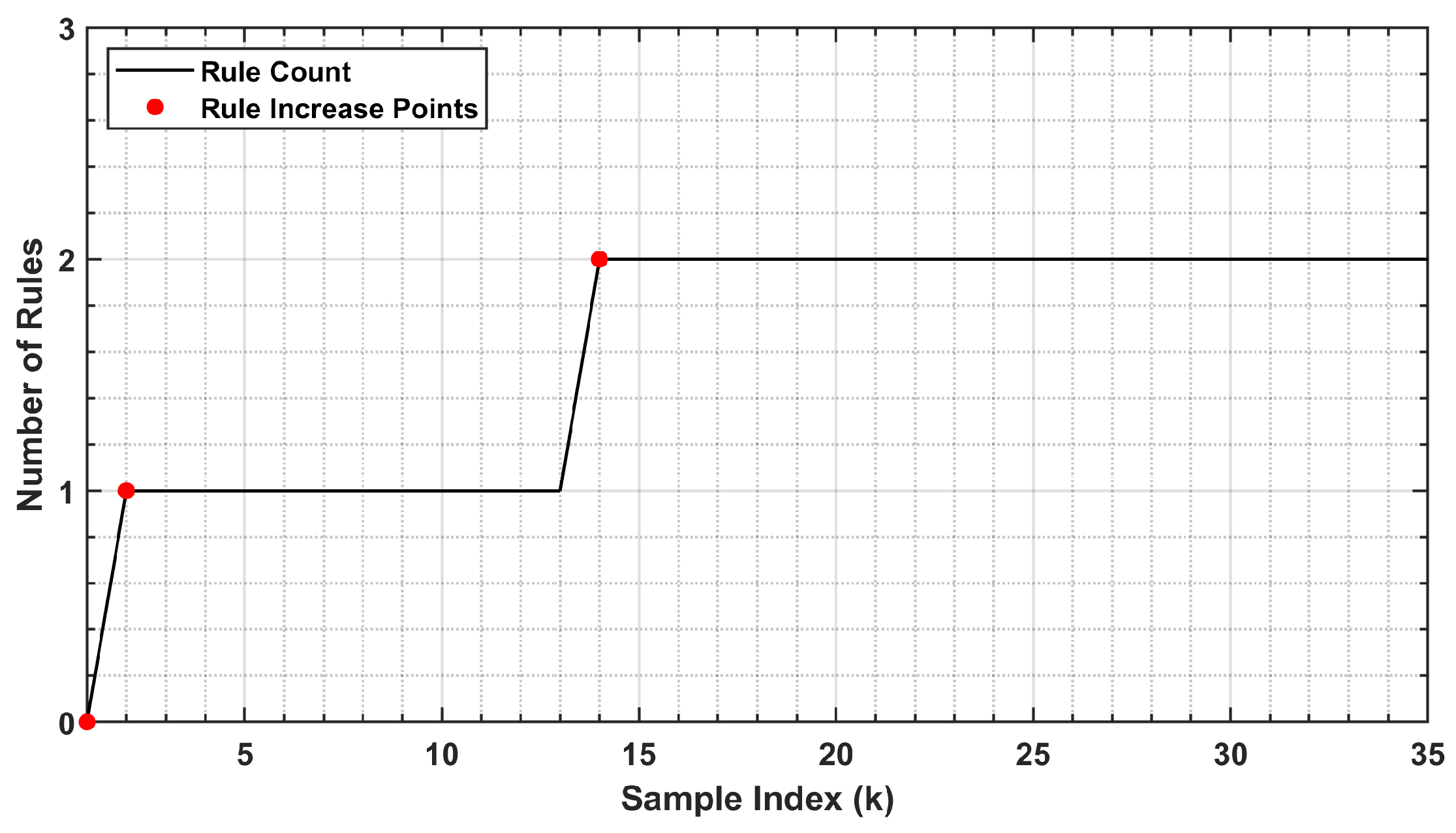
This criterion ensures that a new rule is added only if the current input shows sufficient uniqueness, either structurally or functionally, compared to what the current rule base can represent. Once this condition is satisfied, a new fuzzy rule is initialized using the current input vector as its center. To enhance its accuracy and coverage, the parameters of the newly created rule are further optimized using the proposed CFA. Figure 2 illustrates the effectiveness of the proposed ADAP mechanism on the same 4-step-ahead prediction task. While the original method generates 16 rules within the first 35 samples (see Figure 1), the ADAP model evolves with only 2 rules over the same period. This demonstrates its ability to selectively trigger rule creation based on both geometric distance and activation strength, which can reduce overfitting and computational load. By preventing redundant rules, ADAP can enhance structural simplicity so as to decrease runtime during online updates. The next subsection presents the proposed CFA optimization approach in detail.

2.3. The Proposed Customized Firefly Algorithm (CFA) for Rule Optimization

Once the ADAP mechanism generates a new rule (as discussed in Section 2.2), the current input vector at time step k, denoted by y ( k ) , is used as an initial center c j of the new rule j. However, directly using this raw input may lead to inaccurate position of rule centers, especially in nonlinear or noisy regions of the input space, such as those seen in Li-ion battery data. To address this limitation and enhance rule quality, a CFA is proposed to optimize the antecedent parameters, including the rule center vector c j and the associated MF width vector σ j .
In general, the standard firefly algorithm (FA) is a swarm intelligence-based optimization method inspired by the flashing behavior of fireflies, where less attractive individuals move toward more attractive (i.e., better-performing) ones [66,67]. In the context of CFA, each firefly represents a candidate fuzzy rule characterized by a center vector c and a scalar width σ . The optimization objective is to minimize the absolute prediction error L for the current input sample y ( k ) at a prediction horizon s, defined by:
L = y ( k + s ) y ^ ( k + s )
Unlike the standard FA that operates globally and runs continuously, the proposed CFA is specifically designed for evolving fuzzy systems and is only triggered when a new rule is generated. It performs a single-pass, localized optimization to fine-tune the parameters of the newly added rule. This localized mechanism aims to improve the accuracy of rule placement and make the optimization scalable for real-time applications. The CFA uses a unique movement strategy that combines two interacting behaviors, as outlined below:
(1)
One-to-one movement: Each candidate firefly compares itself with other candidates with lower prediction errors and moves toward them. This allows the candidate to improve by learning from better solutions in its local population.
(2)
Global guidance: Each firefly is softly attracted to the best-performing candidate found so far. This introduces a global guidance to improve convergence and stabilize the search toward a better solution.
The processes can be described by the movement formula of firefly A under the influence of a better-performing firefly B, for updating the center:
c A ( t + 1 ) = c A ( t ) + β A B   e λ D 2 ( c B ( t ) c A ( t ) ) + α · ε
and for updating the width:
σ A ( t + 1 ) = σ A ( t ) + β A B   e λ D 2 ( σ B ( t ) σ A ( t ) ) + α · ε
where c A ( t ) and σ A ( t ) represent the center and width of candidate firefly A at iteration t, while c B ( t ) and σ B ( t ) refer to the corresponding values of a better-performing candidate B. The term D = c A t c B t denotes the Euclidean distance between their centers. The parameter λ = 1 is the light absorption coefficient that controls how distance influences the attractiveness between fireflies. α is a constant that scales a random adjustment ε [ 1 , 1 ] , to maintain diversity in the search so as to avoid trapping in poor solutions. t is the current optimization iteration. β A B is the adaptive attractiveness factor of firefly A toward firefly B, which explained below.
The CFA introduces a novel adaptive attractiveness mechanism, to further improve the optimization process. Rather than using a fixed attractiveness value as in the standard FA, the strength of attraction is adaptively adjusted based on prediction performance:
β A B = β 0 ·   1 L B L A + L B
where β 0 denotes the attractiveness at the initial distance D = 0; L A and L B are the prediction errors of fireflies A and B, respectively.
This adaptive formulation ensures that better-performing fireflies have a stronger influence during movement, which allows them to guide others with higher prediction errors. As a result, the search moves toward more promising regions while maintaining flexibility to continue exploring. This balance between exploration and exploitation allows the CFA to converge more quickly and avoid becoming trapped in poor or noise-affected solutions. The proposed CFA method is to improve the accuracy of newly generated rules without global optimization, which is time consuming. By refining the antecedent parameters locally through adaptive attractiveness, CFA is designed to enhance prediction accuracy while ensuring online training efficiency.
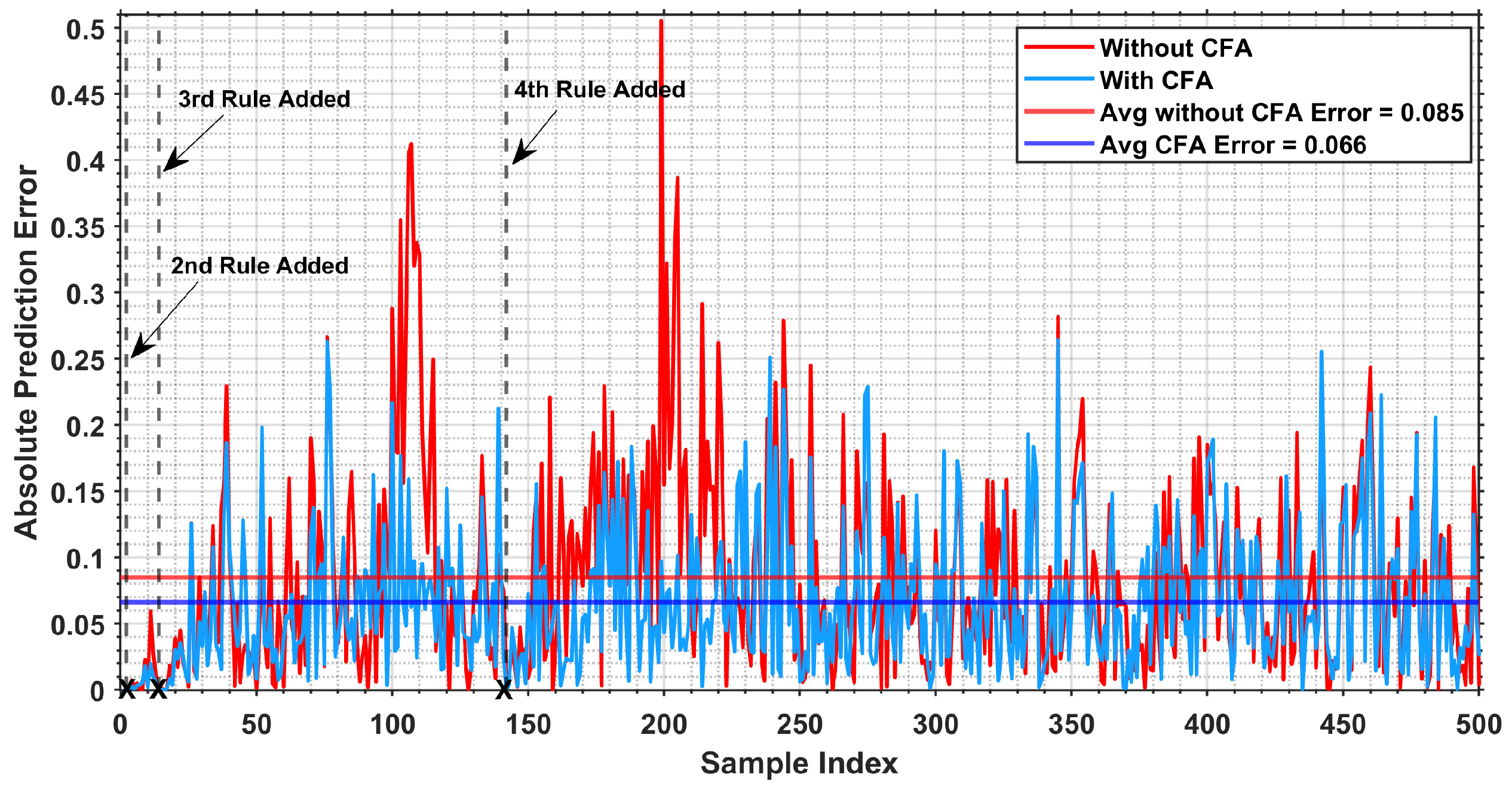
The CFA optimization process runs for a limited number of iterations (e.g., t = 10), during which each firefly candidate updates its rule center and width based on the guided movement strategy. After completing the iterations, the candidate with the lowest prediction error is selected to define the new rule, which is then integrated effectively into the existing model structure. Figure 3 presents a comparison of the absolute prediction error over 500 data samples for both CFA-optimized and non-optimized scenarios, using a 4-steps-ahead prediction task using the Mackey-Glass benchmark under a high level of additive Gaussian noise (standard deviation = 0.12). The results illustrate the importance of optimizing the initial parameters of newly generated rules to ensure they are well-aligned with the current input space, which is important particularly in noisy environments.

3. Simulation Results and Performance Evaluation

The effectiveness of the proposed SEFP-FO technique is evaluated through simulation tests using a benchmark dataset. It is then implemented for battery RUL prediction. The benchmark analysis focuses on prediction accuracy, rule compactness, and adaptability under various conditions, while the battery test demonstrates the model’s practical value in real-world prognostics.

3.1. Simulation Tests Using Benchmark Datasets

This test uses the well-known Mackey-Glass chaotic time series benchmark datasets to evaluate the proposed SEFP-FO technique. A Mackey-Glass dataset is known for its nonlinear dynamics and chaotic behavior, which presents a real challenge for prediction models [48,50,53,58,59]. The simulations assess the model’s performance in terms of prediction accuracy, rule evolution, and reliability across different prediction steps and noise levels. The Mackey-Glass data is described by the following delay differential equation:
d x ( t ) d t = 0.2 x ( t Δ ) 1 + x 10 ( t Δ ) 0.1 x ( t )
In this testing, 10,000 data points are generated with the following conditions: x ( 0 ) = 1.2 , d t = 1 , and Δ = 30 . The proposed SEFP-FO uses equal weighting factors w1 = w2 = 0.50 and a small penalty gain γ = 0.0135. The CFA optimization employs a modest configuration with 20 fireflies and 10 iterations. Two widely accepted evolving fuzzy predictors are used for comparison: the evolving Takagi-Sugeno (eTS) technique based on potential criteria [53] and the distance-based evolving fuzzy system (eFS) technique [58]. All techniques are trained and tested using the same Mackey-Glass datasets, with 8750 samples for training and 1000 samples for testing, to ensure a fair and consistent comparison.

3.1.1. Performance Evaluation for Long-Term Predictions Under Strong Nonlinearity

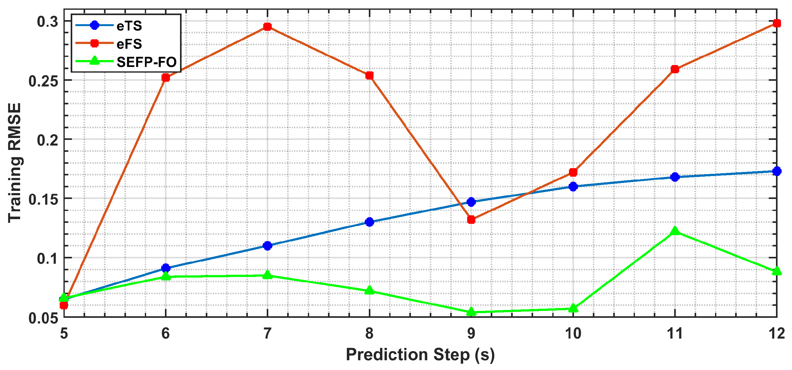
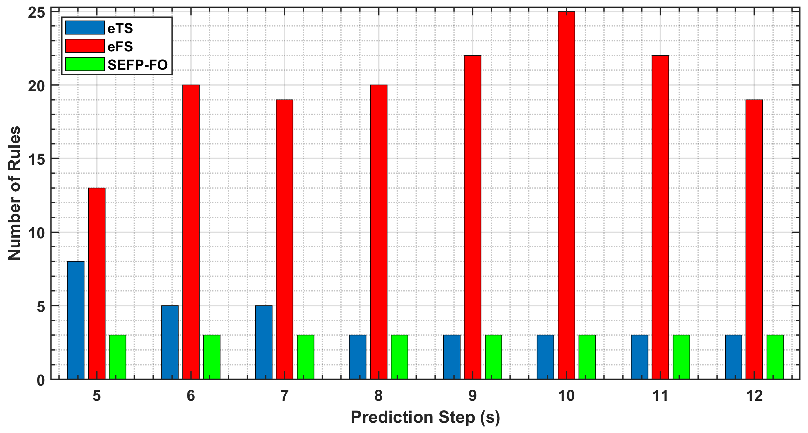
This test is performed to evaluate the long-term prediction accuracy and structural efficiency of the proposed SEFP-FO technique under strong nonlinearity conditions. To fairly assess each technique’s ability to learn and generalize complex nonlinear dynamics, this test uses a noise-free Mackey-Glass dataset with a longer time delay of Δ = 30 , to make the time series more chaotic and challenging than the commonly used setting (e.g., Δ = 17 ). This condition is intentionally chosen to examine the models capability to handle highly nonlinear patterns without the influence of external noise. In this test, prediction accuracy is measured using the root-mean-square error (RMSE), where lower RMSE values indicate better performance. Also, model compactness is evaluated based on the number of fuzzy rules created during training. Because evolving fuzzy systems are updated online, a smaller rule base usually requires less computation per update. Table 2 summarizes the performance of the three techniques (i.e., eTS, eFS, and the proposed SEFP-FO) across multi-step prediction from s = 5 to 12, presenting both training and testing RMSE, as well as the number of rules. Training RMSE is also included to measure overfitting or underfitting when relevant. For instance, comparing training and testing RMSE values can indicate whether a model achieves generalization (close agreement), or suffers from underfitting (consistently high values) or overfitting (large gaps between training and testing errors). Figure 4 presents the training RMSE across prediction steps (s = 5 to 12) using the related techniques. Figure 5 shows the corresponding testing RMSE trends using the three techniques. Figure 6 provides a bar chart comparing the number of fuzzy rules (i.e., model complexity) at each prediction step.
It is seen that the proposed SEFP-FO consistently maintains low training and testing RMSE across all prediction steps, with a compact rule base. For example, at prediction step s = 6, SEFP-FO achieves a lower training RMSE of 0.084 and a testing RMSE of 0.085. The close agreement indicates strong generalization without clear overfitting or underfitting. In comparison, eTS records 0.091/0.093, where both errors remain relatively high, reflecting underfitting. By contrast, eFS has 0.252/0.114, where the large gap between training and testing errors suggests overfitting caused by excessive rule growth. This means that the proposed SEFP-FO can reduce the training RMSE by about 65% and the testing RMSE by 25% compared to eFS and improve the testing RMSE over eTS by around 10%. It also achieves this superior performance using fewer rules than both eTS (i.e., 3 vs. 5) and eFS (i.e., 3 vs. 20) because its efficient ADAP mechanism can help avoid adding redundant or uninformative rules while maintaining high accuracy. Overall, SEFP-FO is compact without losing accuracy because ADAP limits unnecessary rule growth, and CFA refines new rules effectively.
This trend continues at s = 8, where SEFP-FO outperforms both techniques with a testing RMSE of 0.071, which is around 45% lower than that of eTS and 60% lower than that of eFS. At s = 10, it achieves a testing RMSE of 0.057, outperforming eTS by 65% and eFS by 25%, again with a much simpler structure. Even at longer prediction horizons such as s = 12, SEFP-FO performs the best, reaching a testing RMSE of 0.092, which is nearly 50% lower than that of eTS and over 70% lower than that of eFS. Although the eFS technique slightly outperforms SEFP-FO at s = 5, with a testing RMSE of 0.060 versus 0.063, this minor gain in accuracy comes at the cost of significantly higher model complexity, with 13 vs. 3 rules. This indicates that eFS may have achieved this lower error at this step by overfitting through excessive rule growth, rather than by learning a simpler generalizable structure. The proposed SEFP-FO generates lower errors and fewer rules and results in higher computation efficiency, which benefits real-world applications.
Overall, these results highlight the properties of how these three evolving models build and update their structures in dealing with strong nonlinearity. The eTS technique relies on potential-based rule generation, which responds to how closely the data is clustered. While this approach may work reasonably well for shorter prediction horizons, it cannot guide rule creation as the system complexity increases. As a result, eTS may produce too few rules, leading to underfitting to capture nonlinear patterns. The eFS techniques, on the other hand, apply a distance-based rule generation with a fixed threshold. Although this helps it capture more detail, it often adds too many rules (20 to 25), even in noise-free data, because it treats small variations as new information. The fixed threshold can add extra rules and degraded generalization. In contrast, the SEFP-FO uses the ADAP mechanism to avoid adding unnecessary rules by checking how active or unique a new data point is before creating a rule. In addition, when a new rule is added, the proposed CFA optimizes its center and spread to capture data nonlinear dynamics more effectively and efficiently. These results demonstrate that the proposed SEFP-FO technique offers a unique balance between predictive accuracy and structural simplicity in handling highly nonlinear systems. The compact structure with fewer rules also reduces runtime cost during each update operation.

3.1.2. Performance Evaluation Under Noisy Conditions

This subsection evaluates the performance of the proposed SEFP-FO technique under noisy conditions. Additive Gaussian noise is applied to the Mackey-Glass dataset using three standard deviation levels: σ = 0.02, 0.05, and 0.10, representing mild, moderate, and high noise, respectively. A fixed random seed is used when generating the noise to ensure a fair comparison across all models. Evaluation is undertaken based on the testing RMSE, along with model compactness via the number of fuzzy rules. The training RMSE is also included to help interpret specific behaviors of overfitting or underfitting when relevant. For example, a low training error combined with a high testing error may indicate overfitting, while high training and testing errors can indicate insufficient model capability. The results are summarized in Table 3, Table 4 and Table 5, and detailed analysis will be provided below under different noise conditions: mild (σ = 0.02), moderate (σ = 0.05), and high (σ = 0.10). Figure 7 provides an overall view of the balance between prediction accuracy and model complexity under the three noise levels. Each point corresponds to a specific prediction step from s = 5 to 12. Across all cases, SEFP-FO is consistently located in the lower-left region, showing it can achieve lower testing errors with fewer rules compared to eTS and eFS. The lower-left placement means SEFP-FO has lower errors with a smaller rule base, which indicates a lower per-update computation cost.
(A).
Performance under mild noise
As shown in Table 3, the proposed SEFP-FO technique consistently maintains low testing RMSE values across all prediction steps, ranging from 0.049 to 0.087 using only 3 to 4 fuzzy rules. In comparison, eFS requires significantly more rules (up to 27) to achieve comparable accuracy, which increases structural complexity, which decreases computational efficiency in online updating. Although the eTS method generally uses fewer rules than eFS, eTS shows increasing testing errors as the prediction horizon becomes longer. It is observed that at prediction step s = 5, the eTS method records a slightly lower testing RMSE than SEFP-FO (0.073 vs. 0.074), because the potential-based rule generation in eTS manages to capture this local structure over the short-term prediction. However, eTS has a more complex model than SEFP-FO (i.e., 5 vs. 3), which translates into greater processing overhead per sample.
As the prediction steps increase, the proposed SEFP-FO outperforms both the eTS and eFS techniques. For example, at s = 9, SEFP-FO achieves a testing RMSE of 0.053 using only 3 rules, while eTS and eFS reach an RMSE of 0.146 and 0.187, using 3 and 23 rules, respectively. This represents an improvement of 64% over eTS and more than 70% over eFS. A similar trend appears at s = 7, where SEFP-FO achieves a testing RMSE of 0.087, outperforming both eTS at 0.113 and eFS at 0.133, again with fewer rules. At s = 10, SEFP-FO reaches 0.062, which is approximately 60% better than eTS (0.159) and around 30% better than eFS (0.090). At a longer prediction horizon (e.g., s = 12), the proposed SEFP-FO has a testing RMSE of 0.060, much better than eTS and eFS at 0.176 and 0.401, respectively. These results confirm that the proposed SEFP-FO achieves higher accuracy with minimal structural complexity, which can reduce the computational cost.
(B).
Performance under moderate noise
As noise levels increase to moderate (σ = 0.05), the differences between the techniques become more noticeable, especially in terms of generalization and reliability, as shown in Table 4. It is seen that the proposed SEFP-FO can provide better performance across all prediction steps, by achieving the lowest testing RMSE and keeping the model structure relatively minimal overall. This compact structure also limits structural complexity, which in turn improves processing efficiency and scalability when the prediction horizon becomes longer. For instance, at s = 6, SEFP-FO achieves a testing RMSE of 0.093 using 5 rules, compared to 0.193 for eTS (using 5 rules) and 0.281 for eFS (using 18 rules). At steps s = 7 and s = 8, the variations in model behavior become more noticeable. The eTS method uses a few rules (3 and 6, respectively), but both its training and testing RMSE remain relatively high (e.g., 0.205 and 0.216 at s = 7). This indicates that the eTS model cannot effectively learn the underlying data pattern under this noise condition due to underfitting.
In contrast, eFS significantly increases its rule base (18 at s = 7 and 25 at s = 8), but its performance cannot be guaranteed. At s = 8, for example, it gives a high training RMSE of 0.196 but a much lower testing RMSE of 0.090. This unusual gap reflects unstable or inconsistent learning behavior due to noise. The underlying reason is that eFS relies on a fixed distance threshold for rule generation. In noisy conditions, many data points are misclassified as novel, leading to excessive rule growth. These noise-affected rules not only generate inconsistency in training and testing processes, but also increase computational costs. On the other hand, the proposed SEFP-FO technique achieves the lowest testing RMSE values of 0.083 and 0.069 at s = 7 and 8, respectively, with moderate training errors and a small rule base (6 and 10 rules). This reflects the effectiveness of the proposed ADAP strategy in regulating rule growth and the CFA optimization in fine-tuning the placement of newly added rules. Together, the proposed SEFP-FO can adapt to the data without overfitting under noisy conditions. Even at the longest prediction step (i.e., s = 12), the SEFP-FO remains competitive, while its testing RMSE slightly increases to 0.106, which outperforms eTS (0.106 vs. 0.133) by around 20% and eFS (0.106 vs. 0.567) by over 80%. Maintaining accuracy with only a compact rule base highlights computation efficiency with fewer updates and operations at each step.
(C).
Performance under high noise
At a higher noise level of σ= 0.10, the impact of noise on each technique learning mechanism becomes more significant. Table 5 summarizes the performance of eTS, eFS, and SEFP-FO techniques. For instance, at s = 6, SEFP-FO achieves a testing RMSE of 0.119 with 6 rules. In contrast, eTS records a much higher error of 0.498 using just 3 rules, a clear indication of underfitting. This weakness is associated with its potential-based rule generation, where potential values are easily modulated by outliers or noise. Without an adaptive control mechanism, eTS is inefficient to cope with noise, which leads to weak generalization especially at longer prediction horizons.
The eFS technique performs better than eTS in terms of prediction accuracy (e.g., 0.200 at s = 6) but at the cost of rapidly increasing model complexity with 19 rules. Because eFS relies on distance-based rule generation with a fixed threshold, under noisy conditions, noisy points may be treated as new patterns, triggering excessive rule generation. This rule explosion not only results in overfitting but also decreases computation efficiency with extra processing overhead. At s = 9, for instance, eFS generates 22 rules and achieves a testing RMSE of 0.111, which shows a clear improvement over eTS (0.436). However, SEFP-FO still performs the best with a lower error of 0.098 and only using 9 rules. Its compactness can reduce calculations per update without sacrificing accuracy.
These comparisons highlight the different learning behaviors of the three evolving methods. The eTS method is prone to underfitting because its potential measure is easily modulated by noise. As a result, it generates very few rules, which are insufficient to capture the nonlinear characteristics of the data. The eFS method has a better adaptive capability than eTS, but its fixed distance threshold makes it highly sensitive to noise. Even minor noisy data can trigger rule creation, which reduces generalization ability and raises computational demand. By contrast, the proposed SEFP-FO technique addresses these problems through its unique approaches: ADAP limits redundant rule creation by checking whether incoming data are already represented, while CFA fine-tunes the related parameters of newly added rules to enhance accuracy. As a result, SEFP-FO can maintain processing accuracy with a compact rule base, which enables it for real-time prognostic applications.
To further examine the effect of the key sensitivity factors of the proposed SEFP-FO technique, additional experiments are conducted by varying the activation–distance weights (w1, w2) within the range [0.3, 0.7] and by adjusting the penalty gain γ by ±10~20% around its initial setting. Under noise-free conditions, these variations lead to only marginal changes in prediction accuracy (within 3~4%), with the rule base remaining unchanged. When noise is introduced, the effect of these parameters on system performance becomes more noticeable, with modest differences in accuracy as the penalty gain γ increases. On the other hand, the SEFP-FO predictor remains stable and compact without excessive rule generation; SEFP-FO still outperforms eTS and eFS. These findings confirm that the baseline settings adopted in this work (w1 = w2 = 0.5, small γ) provide a better balance to ensure desirable accuracy and efficiency without fine-tuning.

3.2. Performance Evaluation for Battery RUL Prediction

In this subsection, the proposed SEFP-FO technique is implemented and evaluated for RUL prediction of Li-ion batteries. The objective is to assess the model’s ability to accurately capture battery degradation behavior and forecast the end-of-life (EOL) point. The evaluation is conducted using the widely accepted benchmark dataset provided by the NASA Ames Prognostics Center of Excellence [68], which has been commonly employed in the literature for validating battery prognostic methods [13,21,23,30]. Battery #5 is selected as the test case. It is cycled under controlled laboratory conditions using a constant discharge current of 2.0 A. Each cycle ends when the battery voltage drops to 2.7 V. The EOL is defined as the cycle when the battery capacity falls to 70% of its initially rated value. To perform the RUL prediction test, the raw capacity data is slightly smoothed to reduce noise and highlight underlying degradation trends. The test is designed to simulate an online prediction scenario, where only partial historical data is available at the time of forecasting, reflecting real-world conditions in which the full degradation trajectory is not yet observed. Specifically, the complete capacity sequence is split at a predefined prediction starting cycle, and all capacity values up to this point are used for model training. To ensure fairness and consistency across all compared techniques (i.e., eTS, eFS, and SEFP-FO), the same data preprocessing steps, input structure, and prediction horizon are applied.
At each prediction starting point, all three techniques are trained independently from scratch using only the available training data up to that point. A fixed multi-step-ahead autoregressive structure is employed to simulate long-term prediction behavior. Each trained model then generates a forward sequence of predicted capacity values, from which the predicted EOL cycle is identified as the point where the forecasted capacity first drops below the 70% threshold (cycle 161 in this case). A prediction is considered accurate if the estimated EOL cycle closely aligns with this reference point. Table 6 presents the predicted EOL cycles using the related techniques. To assess the long-term prediction accuracy and reliability of each technique, the analysis considers four distinct prediction starting points: cycles 81, 101, 121, and 141. These points reflect different stages of the battery degradation process, ranging from early-life to near-EOL conditions. In each case, the table also summarizes the absolute prediction errors (in cycles), the relative error (%), and the testing RMSE between the predicted and actual capacity values. Figure 8 further summarizes these results by plotting the absolute EOL prediction error (in cycles) against the prediction starting cycle for all related techniques. The clear downward trend confirms that prediction accuracy improves as the starting point moves closer to EOL, with SEFP-FO consistently achieving the lowest error at every stage.
Across all prediction starting points, the proposed SEFP-FO consistently achieves the lowest relative error and testing RMSE, showing higher accuracy in forecasting the battery EOL cycle. At the earliest prediction stage (cycle 81), when little degradation information is available, SEFP-FO predicts the EOL at cycle 144 with a relative error of 10.56%. In comparison, eTS underestimates the EOL at cycle 133 (17.39% error), while eFS fails to produce a valid forecast due to insufficient clustering and rule evolution. This early-stage gap highlights the inherent challenge of making reliable long-term forecasts when degradation data is limited. Figure 9 illustrates the prediction scenario starting at cycle 101. At this stage, the available data reflects part of the battery’s mid-life degradation trend, but accurate long-term forecasting remains a challenging task. SEFP-FO predicts the EOL at cycle 152, just 9 cycles earlier than the true EOL, with a relative error of 5.59% and a low RMSE of 0.025. Also, its prediction curve closely follows the actual capacity decline up to the EOL threshold. Although eTS provides a reasonable estimate at cycle 148 (8.07% error, RMSE = 0.030), it is still less accurate than SEFP-FO. In contrast, eFS generates a poor performance, predicting the EOL at cycle 130 (19.25% error, RMSE = 0.180) and clearly drifting away from the actual trend.
As the prediction starting point moves closer to EOL, all methods benefit from having more representative degradation information. For example, at cycle 121, SEFP-FO achieves a relative error of 4.35% and a testing RMSE of 0.020, outperforming eTS (6.21%, 0.022 RMSE) and eFS (13.66%, 0.114 RMSE). At cycle 141, the SEFP-FO prediction nearly matches the true EOL (160 vs. 161), with just 1 cycle of error and a low RMSE of 0.008. eTS also improves significantly in this case, with 1.86% errors, while eFS is still behind with 6.21% errors. Overall, the SEFP-FO advantage comes from its ability to adapt rule structures dynamically through ADAP and optimize them via the proposed CFA. This combination allows its model to capture the underlying degradation trends more accurately, regardless of how much historical data is available. In contrast, the weaker performance of eFS, especially in early-life predictions, is mainly due to its reliance on distance-based rule creation and lacks a robust mechanism to control rule growth when data is noisy or incomplete. While eTS performs better than eFS in most cases, it still falls short of SEFP-FO, as its potential-based rule evolution can underfit when faced with sudden changes in degradation behavior.
These findings indicate that the proposed SEFP-FO has several advantages that are highly relevant for real applications. Its compact and adaptive structure allows for efficient operation in battery health management. It provides reliable end-of-life forecasts and supports real-time maintenance planning to reduce the risk of unexpected failures. Its robustness to noisy measurements also helps prevent false alarms and improves performance reliability under real operating conditions. Consequently, the proposed SEFP-FO has potential to be used for real-world battery health monitoring and prognostics. These results also confirm the research questions raised in the Introduction that SEFP-FO can achieve high accuracy with a compact rule base, ADAP can effectively control rule growth without degrading accuracy, and the integration of ADAP and CFA mechanisms can improve robustness under noisy test conditions.

4. Conclusions

This work presents a smart evolving fuzzy predictor with customized firefly-based optimization, SEFP-FO, for battery RUL prediction. A novel activation- and distance-aware penalization, ADAP, strategy is proposed to guide rule creation and adaptation. A customized firefly algorithm, CFA, is suggested to optimize newly generated rule parameters. When new rules are added, ADAP learns new patterns with the reuse of existing knowledge. CFA fine-tunes the new rule as soon as it is created to ensure it fits current conditions and is well positioned in the input space. The SEFP-FO technique has a compact structure and adapts to new data patterns effectively. The effectiveness of SEFP-FO is first validated through extensive simulations on benchmark models. Simulation tests show that the SEFP-FO can consistently achieve better performance with lower prediction errors than the other related techniques, using fewer rules and maintaining high performance even under noisy conditions over long-term predictions. The proposed SEFP-FO is also implemented and tested for the battery RUL prediction using the NASA dataset. The test results show that SEFP-FO can achieve accurate and consistent EOL predictions across different prediction starting points. SEFP-FO can improve long-term prediction reliability without increasing model complexity. Future work will be undertaken to explore the application of the SEFP-FO technique to other types of battery chemistries and varying operating conditions, with a more detailed runtime analysis to be considered. Other machine learning and/or deep learning algorithms will be explored to enhance RUL prediction for real electric vehicle applications.

Author Contributions

Conceptualization, M.A.; methodology, M.A. and W.W.; validation, M.A. and W.W.; formal analysis, M.A. and W.W.; investigation, M.A. and W.W.; resources, W.W.; data curation, M.A.; writing—original draft preparation, M.A.; writing—review and editing, M.A. and W.W.; supervision, W.W.; funding acquisition, W.W. All authors have read and agreed to the published version of the manuscript.

Funding

This research received no external funding.

Data Availability Statement

The data presented in this study are openly available in the NASA Ames Prognostics Center of Excellence at https://phm-datasets.s3.amazonaws.com/NASA/5.+Battery+Data+Set.zip, accessed on 1 May 2024 [68].

Acknowledgments

This project was partially supported by the Natural Sciences and Engineering Research Council of Canada (NSERC), eMech Systems Inc., and Bare Point Water Treatment Plant in Thunder Bay, ON, Canada.

Conflicts of Interest

The authors declare no conflicts of interest.

Abbreviations

The following abbreviations are used in this manuscript:
RULRemaining useful life
Li-ionLithium-ion
SEFP-FO Smart evolving fuzzy predictor with customized firefly optimization
EOLEnd-of-life
PFsParticle filters
SOHState-of-health
eFSevolving fuzzy system
ADAPActivation- and distance-aware penalization
FAFirefly algorithm
CFACustomized firefly algorithm
TS-1First-order Takagi-Sugeno
MFsMembership functions
RLSERecursive least squares estimator
RMSERoot-mean-square error
eTSevolving Takagi-Sugeno
NASANational Aeronautics and Space Administration

References

  1. Wang, J.; Liu, P.; Yi, T.; Zhang, J.; Zhang, C. A review on modeling of lithium-ion batteries for electric vehicles. Renew. Sustain. Energy Rev. 2016, 64, 106–128. [Google Scholar] [CrossRef]
  2. Luo, X.; Wang, J.; Dooner, M.; Clarke, J. Overview of current development in electrical energy storage technologies and the application potential in power system operation. Appl. Energy 2015, 137, 511–536. [Google Scholar] [CrossRef]
  3. Ge, M.-F.; Liu, Y.; Jiang, X.; Liu, J. A review on state of health estimations and remaining useful life prognostics of lithium-ion batteries. Measurement 2021, 174, 109057. [Google Scholar] [CrossRef]
  4. Xiong, R.; Pan, Y.; Shen, W.; Li, H.; Sun, F. Lithium-ion battery aging mechanisms and diagnosis method for automotive applications: Recent advances and perspectives. Renew. Sustain. Energy Rev. 2020, 131, 110048. [Google Scholar] [CrossRef]
  5. Wang, Y.; Tian, J.; Sun, Z.; Wang, L.; Xu, R.; Li, M.; Chen, Z. A comprehensive review of battery modeling and state estimation approaches for advanced battery management systems. Renew. Sustain. Energy Rev. 2020, 131, 110015. [Google Scholar] [CrossRef]
  6. Kordestani, M.; Saif, M.; Orchard, M.E.; Razavi-Far, R.; Khorasani, K. Failure prognosis and applications—A survey of recent literature. IEEE Trans. Reliab. 2019, 70, 728–748. [Google Scholar] [CrossRef]
  7. Elmahallawy, M.; Elfouly, T.; Alouani, A.; Massoud, A.M. A Comprehensive Review of Lithium-Ion Batteries Modeling, and State of Health and Remaining Useful Lifetime Prediction. IEEE Access 2022, 10, 119040–119070. [Google Scholar] [CrossRef]
  8. Li, Y.; Liu, K.; Foley, A.M.; Zülke, A.; Berecibar, M.; Nanini-Maury, E.; Van Mierlo, J.; Hoster, H.E. Data-driven health estimation and lifetime prediction of lithium-ion batteries: A review. Renew. Sustain. Energy Rev. 2019, 113, 109254. [Google Scholar] [CrossRef]
  9. Dong, H.; Hu, Q.; Li, D.; Li, Z.; Song, Z. Predictive battery thermal and energy management for connected and automated electric vehicles. IEEE Trans. Intell. Transp. Syst. 2024, 26, 2144–2156. [Google Scholar] [CrossRef]
  10. Reza, M.; Mannan, M.; Mansor, M.; Ker, P.J.; Mahlia, T.M.I.; Hannan, M. Recent advancement of remaining useful life prediction of lithium-ion battery in electric vehicle applications: A review of modelling mechanisms, network configurations, factors, and outstanding issues. Energy Rep. 2024, 11, 4824–4848. [Google Scholar] [CrossRef]
  11. Liu, X.; Hu, Z.; Wang, X.; Xie, M. Capacity Degradation Assessment of Lithium-Ion Battery Considering Coupling Effects of Calendar and Cycling Aging. IEEE Trans. Autom. Sci. Eng. 2023, 21, 3052–3064. [Google Scholar] [CrossRef]
  12. Seaman, A.; Dao, T.-S.; McPhee, J. A survey of mathematics-based equivalent-circuit and electrochemical battery models for hybrid and electric vehicle simulation. J. Power Sources 2014, 256, 410–423. [Google Scholar] [CrossRef]
  13. Ahwiadi, M.; Wang, W. An AI-driven particle filter technology for battery system state estimation and RUL prediction. Batteries 2024, 10, 437. [Google Scholar] [CrossRef]
  14. Meng, H.; Li, Y.-F. A review on prognostics and health management (PHM) methods of lithium-ion batteries. Renew. Sustain. Energy Rev. 2019, 116, 109405. [Google Scholar] [CrossRef]
  15. Ahwiadi, M.; Wang, W. Battery Health Monitoring and Remaining Useful Life Prediction Techniques: A Review of Technologies. Batteries 2025, 11, 31. [Google Scholar] [CrossRef]
  16. Hu, X.; Xu, L.; Lin, X.; Pecht, M. Battery Lifetime Prognostics. Joule 2020, 4, 310–346. [Google Scholar] [CrossRef]
  17. Beelen, H.; Bergveld, H.J.; Donkers, M.C.F. Joint Estimation of Battery Parameters and State of Charge Using an Extended Kalman Filter: A Single-Parameter Tuning Approach. IEEE Trans. Control. Syst. Technol. 2020, 29, 1087–1101. [Google Scholar] [CrossRef]
  18. He, H.; Qin, H.; Sun, X.; Shui, Y. Comparison study on the battery SoC estimation with EKF and UKF algorithms. Energies 2013, 6, 5088–5100. [Google Scholar] [CrossRef]
  19. Partovibakhsh, M.; Liu, G. An Adaptive Unscented Kalman Filtering Approach for Online Estimation of Model Parameters and State-of-Charge of Lithium-Ion Batteries for Autonomous Mobile Robots. IEEE Trans. Control. Syst. Technol. 2014, 23, 357–363. [Google Scholar] [CrossRef]
  20. Zhang, S.; Guo, X.; Zhang, X. An improved adaptive unscented kalman filtering for state of charge online estimation of lithium-ion battery. J. Energy Storage 2020, 32, 101980. [Google Scholar] [CrossRef]
  21. Ahwiadi, M.; Wang, W. An Adaptive Particle Filter Technique for System State Estimation and Prognosis. IEEE Trans. Instrum. Meas. 2020, 69, 6756–6765. [Google Scholar] [CrossRef]
  22. Saha, B.; Goebel, K. Modeling Li-ion battery capacity depletion in a particle filtering framework. In Proceedings of the Annual Conference of the Prognostics and Health Management Society, San Diego, CA, USA, 27 September–1 October 2009; pp. 1–10. [Google Scholar]
  23. Saha, B.; Goebel, K.; Poll, S.; Christophersen, J. An integrated approach to battery health monitoring using Bayesian regression and state estimation. In Proceedings of the IEEE Autotestcon, Baltimore, MD, USA, 17–20 September 2007; pp. 646–653. [Google Scholar]
  24. Li, D.Z.; Wang, W.; Ismail, F. A mutated particle filter technique for system state estimation and battery life prediction. IEEE Trans. Instrum. Meas. 2014, 63, 2034–2043. [Google Scholar] [CrossRef]
  25. Tian, Y.; Lu, C.; Wang, Z.; Tao, L. Artificial Fish Swarm Algorithm-Based Particle Filter for Li-Ion Battery Life Prediction. Math. Probl. Eng. 2014, 2014, 564894. [Google Scholar] [CrossRef]
  26. Liu, D.; Luo, Y.; Liu, J.; Peng, Y.; Guo, L.; Pecht, M. Lithium-ion battery remaining useful life estimation based on fusion nonlinear degradation AR model and RPF algorithm. Neural Comput. Appl. 2013, 25, 557–572. [Google Scholar] [CrossRef]
  27. Ren, Y.; Tang, T.; Xia, Q.; Zhang, K.; Tian, J.; Hu, D.; Yang, D.; Sun, B.; Feng, Q.; Qian, C. A data and physical model joint driven method for lithium-ion battery remaining useful life prediction under complex dynamic conditions. J. Energy Storage 2024, 79, 110065. [Google Scholar] [CrossRef]
  28. Zhang, C.; Zhao, S.; He, Y. An Integrated Method of the Future Capacity and RUL Prediction for Lithium-Ion Battery Pack. IEEE Trans. Veh. Technol. 2021, 71, 2601–2613. [Google Scholar] [CrossRef]
  29. Tian, H.; Qin, P.; Li, K.; Zhao, Z. A review of the state of health for lithium-ion batteries: Research status and suggestions. J. Clean. Prod. 2020, 261, 120813. [Google Scholar] [CrossRef]
  30. Du, Z.; Zuo, L.; Li, J.; Liu, Y.; Shen, H.T. Data-Driven Estimation of Remaining Useful Lifetime and State of Charge for Lithium-Ion Battery. IEEE Trans. Transp. Electrif. 2021, 8, 356–367. [Google Scholar] [CrossRef]
  31. Nuhic, A.; Terzimehic, T.; Soczka-Guth, T.; Buchholz, M.; Dietmayer, K. Health diagnosis and remaining useful life prognostics of lithium-ion batteries using data-driven methods. J. Power Sources 2013, 239, 680–688. [Google Scholar] [CrossRef]
  32. Khosravi, A.; Nahavandi, S.; Creighton, D.; Atiya, A. A Comprehensive Review of Neural Network-based Prediction Intervals and New Advances. IEEE Trans. Neural Netw. 2011, 22, 1341–1356. [Google Scholar] [CrossRef]
  33. Wang, S.; Wang, Z.; Pan, J.; Zhang, Z.; Cheng, X. A data-driven fault tracing of lithium-ion batteries in electric vehicles. IEEE Trans. Power Electron. 2024, 39, 16609–16621. [Google Scholar] [CrossRef]
  34. Catelani, M.; Ciani, L.; Fantacci, R.; Patrizi, G.; Picano, B. Remaining Useful Life Estimation for Prognostics of Lithium-Ion Batteries Based on Recurrent Neural Network. IEEE Trans. Instrum. Meas. 2021, 70, 3524611. [Google Scholar] [CrossRef]
  35. Zheng, X.; Deng, X. State-of-Health Prediction For Lithium-Ion Batteries With Multiple Gaussian Process Regression Model. IEEE Access 2019, 7, 150383–150394. [Google Scholar] [CrossRef]
  36. Wang, Y.; Ni, Y.; Lu, S.; Wang, J.; Zhang, X. Remaining Useful Life Prediction of Lithium-Ion Batteries Using Support Vector Regression Optimized by Artificial Bee Colony. IEEE Trans. Veh. Technol. 2019, 68, 9543–9553. [Google Scholar] [CrossRef]
  37. Abdolrasol, M.G.M.; Ayob, A.; Lipu, M.S.H.; Ansari, S.; Kiong, T.S.; Saad, M.H.M.; Ustun, T.S.; Kalam, A. Advanced data-driven fault diagnosis in lithium-ion battery management systems for electric vehicles: Progress, challenges, and future perspectives. eTransportation. 2024, 22, 100374. [Google Scholar] [CrossRef]
  38. Qu, J.; Liu, F.; Ma, Y.; Fan, J. A Neural-Network-Based Method for RUL Prediction and SOH Monitoring of Lithium-Ion Battery. IEEE Access 2019, 7, 87178–87191. [Google Scholar] [CrossRef]
  39. Zhou, D.; Li, Z.; Zhu, J.; Zhang, H.; Hou, L. State of Health Monitoring and Remaining Useful Life Prediction of Lithium-Ion Batteries Based on Temporal Convolutional Network. IEEE Access 2020, 8, 53307–53320. [Google Scholar] [CrossRef]
  40. Zraibi, B.; Okar, C.; Chaoui, H.; Mansouri, M. Remaining Useful Life Assessment for Lithium-Ion Batteries Using CNN-LSTMDNN Hybrid Method. IEEE Trans. Veh. Technol. 2021, 70, 4252–4261. [Google Scholar] [CrossRef]
  41. Li, Y.; Li, L.; Mao, R.; Zhang, Y.; Xu, S.; Zhang, J. Hybrid Data-Driven Approach for Predicting the Remaining Useful Life of Lithium-Ion Batteries. IEEE Trans. Transp. Electrif. 2023, 10, 2789–2805. [Google Scholar] [CrossRef]
  42. Cartagena, O.; Parra, S.; Muñoz-Carpintero, D.; Marín, L.G.; Sáez, D. Review on Fuzzy and Neural Prediction Interval Modelling for Nonlinear Dynamical Systems. IEEE Access 2021, 9, 23357–23384. [Google Scholar] [CrossRef]
  43. Jafari, S.; Byun, Y.C. A CNN-GRU Approach to the Accurate Prediction of Batteries’ Remaining Useful Life from Charging Profiles. Computers 2023, 12, 219. [Google Scholar] [CrossRef]
  44. He, W.; Li, Z.; Liu, T.; Liu, Z.; Guo, X.; Du, J.; Li, X.; Sun, P.; Ming, W. Research progress and application of deep learning in remaining useful life, state of health and battery thermal management of lithium batteries. J. Energy Storage 2023, 70, 107868. [Google Scholar] [CrossRef]
  45. Oji, T.; Zhou, Y.; Ci, S.; Kang, F.; Chen, X.; Liu, X. Data-driven methods for battery soh estimation: Survey and a critical analysis. IEEE Access 2021, 10, 126903–126916. [Google Scholar] [CrossRef]
  46. Škrjanc, I.; Iglesias, J.A.; Sanchis, A.; Leite, D.; Lughofer, E.; Gomide, F. Evolving fuzzy and neuro-fuzzy approaches in clustering, regression, identification, and classification: A survey. Inf. Sci. 2019, 490, 344–368. [Google Scholar] [CrossRef]
  47. Lughofer, E.; Skrjanc, I. Evolving Error Feedback Fuzzy Model for Improved Robustness under Measurement Noise. IEEE Trans. Fuzzy Syst. 2022, 31, 997–1008. [Google Scholar] [CrossRef]
  48. Ahwiadi, M.; Wang, W. An Adaptive Evolving Fuzzy Technique for Prognosis of Dynamic Systems. IEEE Trans. Fuzzy Syst. 2021, 30, 841–849. [Google Scholar] [CrossRef]
  49. Juang, C.F.; Tsao, Y.W. A Self-evolving interval type-2 fuzzy neural network with online structure and parameter learning. IEEE Trans. Fuzzy Syst. 2008, 16, 1411–1424. [Google Scholar] [CrossRef]
  50. Angelov, P.; Buswell, R. Identification of evolving rule-based models. IEEE Trans. Fuzzy Syst. 2002, 10, 667–677. [Google Scholar] [CrossRef]
  51. Angelov, P.; Filev, D.P. An approach to online identification of Takagi-Sugeno fuzzy models. IEEE Trans. Syst. Man Cybern. Part B 2004, 34, 484–498. [Google Scholar] [CrossRef]
  52. Angelov, P. Fuzzily connected multimodel systems evolving autonomously from data streams. IEEE Trans. Syst. Man Cybern. Part B 2011, 41, 898–910. [Google Scholar] [CrossRef]
  53. Wang, W.; Li, D.Z.; Vrbanek, J. An evolving neuro-fuzzy technique for system state forecasting. Neurocomputing 2012, 87, 111–119. [Google Scholar] [CrossRef]
  54. Lughofer, E.D. FLEXFIS: A robust incremental learning approach for evolving Takagi–Sugeno fuzzy models. IEEE Trans. Fuzzy Syst. 2008, 16, 1393–1410. [Google Scholar] [CrossRef]
  55. Li, D.; Wang, W.; Ismail, F. An evolving fuzzy neural predictor for multi-dimensional system state forecasting. Neurocomputing 2014, 145, 381–391. [Google Scholar] [CrossRef]
  56. Lughofer, E.; Cernuda, C.; Kindermann, S.; Pratama, M. Generalized smart evolving fuzzy systems. Evol. Syst. 2015, 6, 269–292. [Google Scholar] [CrossRef]
  57. Maciel, L.; Ballini, R.; Gomide, F. An evolving possibilistic fuzzy modeling approach for value-at-risk estimation. Appl. Soft Comput. 2017, 60, 820–830. [Google Scholar] [CrossRef]
  58. Wang, W.; Vrbanek, J. An evolving fuzzy predictor for industrial applications. IEEE Trans. Fuzzy Syst. 2008, 16, 1439–1449. [Google Scholar] [CrossRef]
  59. Ge, D.; Zeng, X.J. Learning data streams online—An evolving fuzzy system approach with self-learning/adaptive thresholds. Inf. Sci. 2020, 507, 172–184. [Google Scholar] [CrossRef]
  60. Nguyen, N.N.; Zhou, W.J.; Quek, C. GSETSK: A generic self-evolving TSK fuzzy neural network with a novel Hebbian-based rule reduction approach. Appl. Soft Comput. 2015, 35, 29–42. [Google Scholar] [CrossRef]
  61. Lughofer, E.; Zavoianu, A.; Pollak, R.; Pratama, M.; Meyer-Heye, P.; Zorrer, H.; Eitzinger, C.; Haim, J.; Radauer, T. Self-adaptive evolving forecast models with incremental PLS space updating for on-line prediction of micro-fluidic chip quality. Eng. Appl. Artif. Intell. 2018, 68, 131–151. [Google Scholar] [CrossRef]
  62. Cartagena, O.; Trovò, F.; Roveri, M.; Sáez, D. Evolving fuzzy prediction intervals in nonstationary environments. IEEE Trans. Emerg. Top. Comput. Intell. 2024, 8, 903–916. [Google Scholar] [CrossRef]
  63. Baruah, R.D.; Angelov, P. DEC: Dynamically evolving clustering and its application to structure identification of evolving fuzzy models. IEEE Trans. Cybern. 2014, 44, 1619–1631. [Google Scholar] [CrossRef]
  64. Mei, Z.; Zhao, T.; Gu, X. A dynamic evolving fuzzy system for streaming data prediction. IEEE Trans. Fuzzy Syst. 2024, 32, 4324–4337. [Google Scholar] [CrossRef]
  65. Angelov, P. Evolving fuzzy systems. In Computational Complexity; Meyers, R.A., Ed.; Springer: New York, NY, USA, 2012; pp. 1053–1065. [Google Scholar]
  66. Yang, X.-S. Firefly algorithms for multimodal optimization. In Stochastic Algorithms: Foundations and Applications; Springer: Berlin, Germany, 2009; Volume 9, pp. 169–178. [Google Scholar]
  67. Li, J.; Wei, X.Y.; Li, B.; Zeng, Z.G. A survey on firefly algorithms. Neurocomputing 2022, 500, 662–678. [Google Scholar] [CrossRef]
  68. Saha, B.; Goebel, K. Battery Data Set. In NASA Prognostics Data Repository; NASA Ames Research Center: Moffett Field, CA, USA, 2024; Available online: https://phm-datasets.s3.amazonaws.com/NASA/5.+Battery+Data+Set.zip (accessed on 1 May 2024).
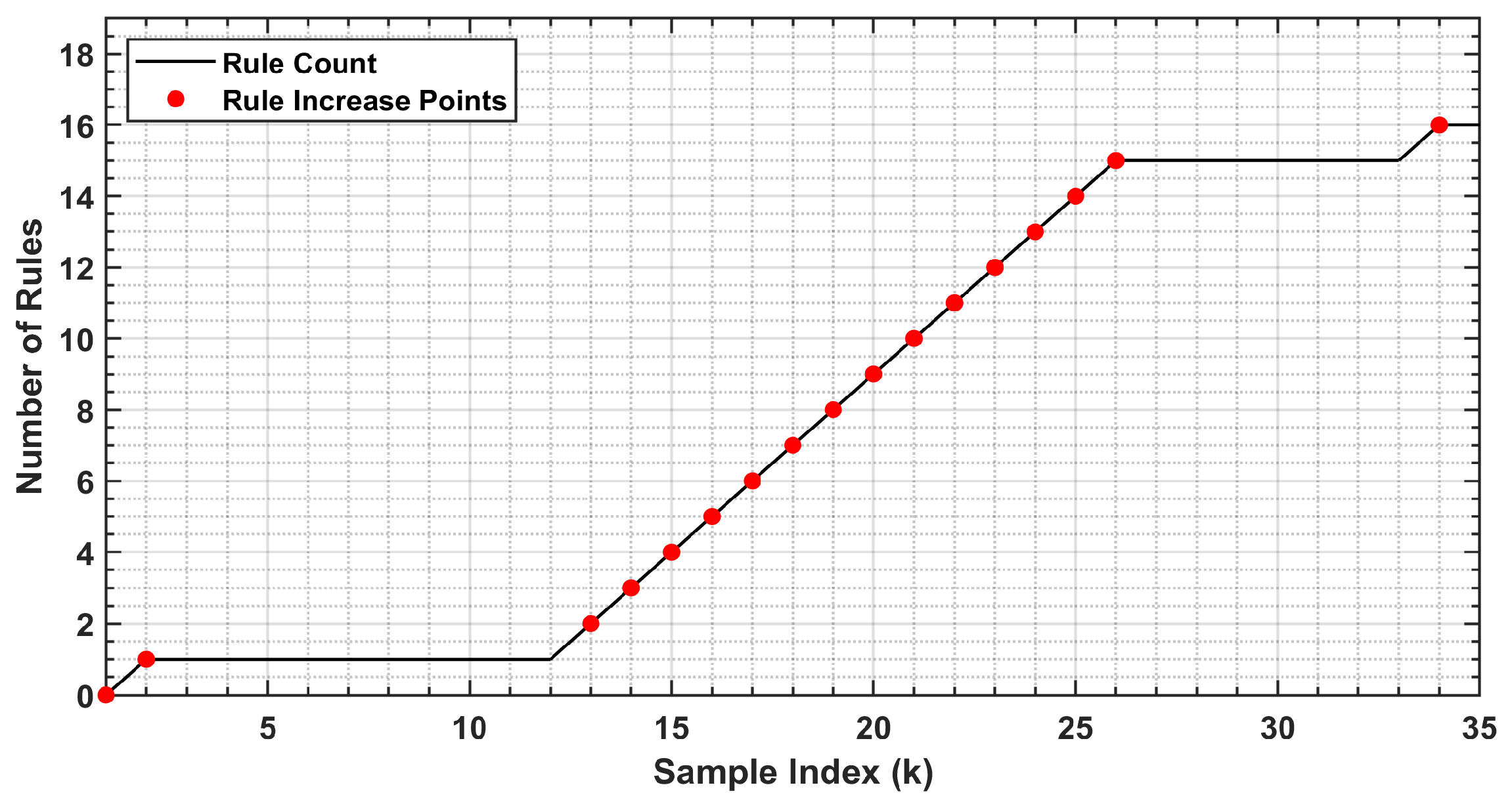
Figure 1. Illustration of rapid rule growth driven by minor statistical variations.
Batteries 11 00362 g001
Figure 2. Illustration of controlled rule evolution using the proposed ADAP method.
Batteries 11 00362 g002
Figure 3. Absolute prediction errors over 500 samples with and without CFA optimization under high noise in a 4-steps-ahead Mackey-Glass prediction task.
Batteries 11 00362 g003
Figure 4. Comparison of training RMSE across prediction steps (s = 5 to 12) using the eTS, eFS, and SEFP-FO techniques.
Batteries 11 00362 g004
Figure 5. Comparison of testing RMSE across prediction steps (s = 5 to 12) using the eTS, eFS, and SEFP-FO techniques.
Batteries 11 00362 g005
Figure 6. Comparison of the number of fuzzy rules (model complexity) across prediction steps (s = 5 to 12) using the eTS, eFS, and SEFP-FO techniques.
Batteries 11 00362 g006
Figure 7. Testing RMSE versus number of rules for eTS, eFS, and SEFP-FO techniques under noise levels: (a) σ = 0.02, (b) σ = 0.05, and (c) σ = 0.10, where each corresponds to a prediction step (s = 5 to 12).
Batteries 11 00362 g007
Figure 8. Absolute EOL prediction error (in cycles) for eTS, eFS, and SEFP-FO across different prediction starting points (81, 101, 121, and 141).
Batteries 11 00362 g008
Figure 9. Predicted capacity using: eTS (blue dotted line), eFS (black dash-dotted line), the proposed SEFP-FO (red dashed line), and the actual capacity (solid green line), for the prediction starting at cycle 101.
Batteries 11 00362 g009
Table 1. Comparative overview of representative approaches.
ApproachAccuracyInterpretabilityAdaptiveness/Online UseRobustness to NoiseComputational Cost
Model-based [9,12,14,15]Good when model is accurateHigh Limited; often fixed parameters; sensitive to assumptionsHandles some noise but sensitive to non-Gaussian errorsModerate–High
Hybrid [16,17,18]Often improved accuracyMediumLimited by integration of componentsSensitive to noise; improved with denoising High
Classical ML [19,20,21]Works well in stable or short-horizon predictionsMediumLow; retraining needed under driftSensitive to noise; limited robustnessLow–Moderate
Deep learning [22,23,24,25]High with large, labeled datasetsLow (“black box”)Low online adaptiveness; prone to overfitting and driftModerate; needs regularizationHigh (training), Moderate (inference)
Evolving fuzzy systems [26,27,28,29,30]Effective on nonlinear, time-varying dataHighHigh; structure evolves onlineMedium; sensitive to thresholds and noiseModerate; costly if many rules created
Table 2. Performance comparison under strong nonlinearity of the related techniques on noise-free Mackey-Glass data.
No. of StepseTSeFSSEFP-FO
Training
RMSE
Testing
RMSE
No. of RulesTraining
RMSE
Testing
RMSE
No. of RulesTraining
RMSE
Testing
RMSE
No. of Rules
50.0650.06380.0600.060130.0660.0633
60.0910.09350.2520.114200.0840.0853
70.1100.11150.2950.278190.0850.0863
80.1300.13230.2540.192200.0720.0713
90.1470.15030.1320.061220.0540.0553
100.1600.16430.1720.076250.0570.0573
110.1680.17630.2590.335220.1220.1293
120.1730.18330.2980.309190.0880.0923
Table 3. Performance comparison of the related techniques under mild noise (σ =0.02) on the noisy Mackey-Glass dataset.
No. of StepseTSeFSSEFP-FO
Training
RMSE
Testing
RMSE
No. of RulesTraining
RMSE
Testing
RMSE
No. of RulesTraining
RMSE
Testing
RMSE
No. of Rules
50.0750.07350.0670.077180.0740.0743
60.0930.09360.3210.338190.0850.0853
70.1100.11330.1690.133220.0860.0873
80.1270.13030.2190.102210.0740.0753
90.1410.14630.2110.187230.0510.0533
100.1530.15930.1550.090270.0600.0623
110.1610.17030.2380.351200.0500.0493
120.1670.17630.2180.401210.0590.0604
Table 4. Performance comparison of the related techniques under moderate noise (σ = 0.05) on the noisy Mackey-Glass dataset.
No. of StepseTSeFSSEFP-FO
Training
RMSE
Testing
RMSE
No. of RulesTraining
RMSE
Testing
RMSE
No. of RulesTraining
RMSE
Testing
RMSE
No. of Rules
50.0870.088110.0840.085170.0890.0894
60.1900.19350.2530.281180.1160.0935
70.2050.21630.1470.172180.1200.0836
80.1280.12160.1960.090250.1060.06910
90.0810.074150.2230.319250.0730.0715
100.1520.07880.1940.101250.1390.0875
110.1930.14980.2110.398230.1190.0716
120.1250.13380.2480.567220.0970.1065
Table 5. Performance comparison under high noise (σ = 0.10) on the Mackey-Glass dataset.
No. of StepseTSeFSSEFP-FO
Training
RMSE
Testing
RMSE
No. of RulesTraining
RMSE
Testing
RMSE
No. of RulesTraining
RMSE
Testing
RMSE
No. of Rules
50.1000.102100.0980.104180.1000.1026
60.2870.49830.2000.200190.1530.1196
70.1910.119160.1960.215170.1340.1077
80.2670.43660.1690.130200.1640.1555
90.2380.43680.1870.111220.1470.0989
100.2600.114160.1680.153240.1290.1018
110.1300.13160.1610.133210.1190.1317
120.1300.13790.2050.193210.1290.1396
Table 6. Battery EOL prediction results using the related techniques at different prediction starting points (true EOL = 161 cycles).
Prediction Starting PointTechniquePrediction Result (Cycle)Error (Cycle)Relative ErrorTesting
RMSE
81eTS1332817.39%0.067
eFS---0.478
SEFP-FO1441710.56%0.031
101eTS148138.07%0.030
eFS1303119.25%0.180
SEFP-FO15295.59%0.025
121eTS151106.21%0.022
eFS1392213.66%0.114
SEFP-FO15474.35%0.020
141eTS15831.86%0.013
eFS151106.21%0.053
SEFP-FO16010.62%0.008
Disclaimer/Publisher’s Note: The statements, opinions and data contained in all publications are solely those of the individual author(s) and contributor(s) and not of MDPI and/or the editor(s). MDPI and/or the editor(s) disclaim responsibility for any injury to people or property resulting from any ideas, methods, instructions or products referred to in the content.