Useful Quantities and Diagram Types for Diagnosis and Monitoring of Electrochemical Energy Converters Using Impedance Spectroscopy: State of the Art, Review and Outlook

Abstract

The concept of pseudocapacitance is explored as a rapid and universal method for the state of health (SOH) determination of batteries and supercapacitors. In contrast to this, the state of the art considers the degradation of a series of full charge/discharge cycles. Lithium-ion batteries, sodium-ion batteries and supercapacitors of different cell chemistries are studied by impedance spectroscopy during lifetime testing. Faradaic and capacitive charge storage are distinguished by the relationship between the stored electric charge and capacitance. Batteries with a flat voltage–charge curve are best suited for impedance spectroscopy. There is a slight loss in the linear correlation between the pseudocapacitance and Ah capacity in regions of overcharge and deep discharge. The correct calculation of quantities related to complex impedance and differential capacitance is outlined, which may also be useful as an introductory text and tutorial for newcomers to the field. Novel diagram types are proposed for the purpose of the instant performance and failure diagnosis of batteries and supercapacitors.

1. Introduction

In-time failure diagnosis is still a challenge for battery management systems with respect to and the reliable indication of the state of charge (SOC) and state of health (SOH) of electrochemical energy storage devices. The current state of the art of lifespan prediction is mostly based on cell voltage monitoring or ampere-hour counting and the evaluation of hundreds of complete charge/discharge cycles. At present, there is no quick and simple method to determine the actual SOC, regardless of the age of the battery. It is still not clear when a battery is truly fully charged during charging without overcharging and when its power is almost depleted during discharging. Various internal and external problems can arise during operation in stationary and mobile applications, leading to performance losses and thermal runaway.

1.1. Scope of This Study

With respect to providing more general insights into the diagnosis of different electrochemical energy converters, the concept of impedance spectroscopy [1] has been verified through examples of lithium-ion cells and supercapacitors during longtime tests. We tested hundreds of lithium-ion batteries of different manufacturers and cell chemistries and considered whether there was a simple means to determine whether they were ‘full’ or ‘empty’ without performing a full charge/discharge cycle each time and risking the overcharge or deep discharge of the cell. It can be challenging to determine the actual SOC and SOH of lithium-ion batteries after they have been idle for a while or after a high-power discharge.

When comparing faradaic and capacitive energy storage, questions arise: How does pseudocapacitance reflect the available electric charge? Which impedance-derived quantity gives the best information on aging, state of health and failure diagnosis? Which early signs indicate thermal overload and critical overcharge in the impedance spectra of batteries that are considered to be in good condition? What is the deep electrochemical information of resistance and capacitance during lifetime testing? This paper aims to provide answers.

1.2. Practical Background

In the aviation sector, the fast charging of batteries is usually not permitted. Even if the battery is fully charged, it cannot be guaranteed that it has sufficient capacity to last for 15 min under a full load during an emergency. Because of the high reliability standards of emergency power supplies in aircraft, planned take-offs can sometimes be delayed. Once the plane is parked, the battery’s state of charge (SOC) drops because of self-discharge. It takes about 1.5 to 2 h to diagnose a 2 Ah battery, determine its capacity, and recharge it using the constant current discharge method, according to the latest in-air traffic technology. If we wish to keep maintenance intervals short, we need a reliable method to diagnose batteries quickly that can at least indicate the upper SOC range.

The cell voltage provides limited information about the remaining capacity and state of health (SOH) of the battery, which is assessed every 6 months during maintenance. Predicting the remaining useful life (RUL) is challenging due to a kink or knee in the degradation curve. As battery replacement is costly and logistically challenging in remote areas, the direct measurement of degradation is preferred.

Lithium iron phosphate (LFP) is known to be less sensitive to thermal runaway and fire in the event of overcharging and overheating than cobalt-based systems (LCO, NMC, NCA) and manganese spinel (LMO). In the olivine lattice of Li_1−xFePO₄, lithium ions move through the linear channels. The LFP material is easy to obtain, does not require much critical attention, and is unlikely to cause any harm. Unfortunately, the cell voltage of 3.6 V is lower than the 4.2 V of most other lithium technologies. The capacity is more likely to degrade if the battery is left running for long periods of time in either the upper or lower potential range and at low temperatures.

Supercapacitors are considered for emergency power supplies [2,3]. Impedance measurements help us to understand the difference between the capacitance C and the differential capacity of a battery, dQ/dU, which is the first derivative of the charge/discharge curve Q(U) [4].

2. Definition of Quantities Related to Complex Impedance

2.1. The Concept of Impedance

Regardless of their type, electronically or ionically conductive materials exhibit complex resistance, known as impedance Z, when subjected to an alternating current of a given frequency [5].

Electrochemical impedance spectroscopy (EIS) [6,7] measures the frequency-dependent resistance and reactance of the device under test. A constant voltage (potentiostatic impedance method) or a constant current (galvanostatic impedance method) is superimposed on an AC voltage or AC current of small amplitude, and the phase shift between the current and voltage is measured. Signal multiplication and averaging separate the useful signal from the DC components, harmonics, and noise. A measurement point takes a multiple of 1/f seconds. To avoid changes in the cell, the impedance spectrum is measured from high to low frequencies (from MHz to mHz). Frequency response analyzers output the complex resistance Z (consisting of a real part and an imaginary part) or impedance value and phase angle (Z, φ) in the frequency domain.

$$\underset{\_}{Z}\left(\mathrm{j}\omega \right)=\frac{\mathcal{F}\left\{U\left(t\right)\right\}}{\mathcal{F}\left\{I\left(t\right)\right\}}=\frac{U\left(\mathrm{j}\omega \right)}{I\left(\mathrm{j}\omega \right)}=\left|\underset{\_}{Z}\left(\mathrm{j}\omega \right)\right|\cdot e^{\mathrm{j}\mathsf{\phi }}=\mathrm{R}\mathrm{e} \underset{\_}{Z}\left(\mathrm{j}\omega \right)+\mathrm{j}\mathrm{}\mathrm{I}\mathrm{m} \underset{\_}{Z}\left(\mathrm{j}\omega \right)$$

(1)

The underscore in Equation (1) indicates that Z is a complex value, while |Z| is the absolute value (modulus) of the impedance (see

Table 1. Definitions of complex quantities related to impedance in mathematical convention.

Quantity	Complex Definition	Real Part Active Component	Imaginary Part Reactive Component	Modulus Apparent Value	Unit
Impedance	$\underset{\_}{Z}\left(\mathrm{j}\omega \right)=\mathrm{R}\mathrm{e} \underset{\_}{Z}+\mathrm{j} \mathrm{I}\mathrm{m} \underset{\_}{Z}$	$R=\mathrm{R}\mathrm{e} \underset{\_}{Z}$	$X=\mathrm{I}\mathrm{m} \underset{\_}{Z}$	$Z=\left|\underset{\_}{Z}\right|=\sqrt{R^2+Z^2}=\frac{U}{I}$	$\mathsf{\Omega }$
Admittance	$\underset{\_}{Y}\left(\mathrm{j}\omega \right)=\mathrm{R}\mathrm{e} \underset{\_}{Y}+\mathrm{j} \mathrm{I}\mathrm{m} \underset{\_}{Y}=\frac{1}{\underset{\_}{Z}\left(\mathrm{j}\omega \right)}$	$G=\frac{\mathrm{R}\mathrm{e} \underset{\_}{Z}}{{\left|\underset{\_}{Z}\right|}^2}$	$B=-\frac{\mathrm{I}\mathrm{m} \underset{\_}{Z}}{{\left|\underset{\_}{Z}\right|}^2}$	$Y=\left|\underset{\_}{Y}\right|=\sqrt{G^2+B^2}=Z^{-1}$	${\mathsf{\Omega }}^{-1}$
Capacitance	$\underset{\_}{C}\left(\mathrm{j}\omega \right)=\mathrm{R}\mathrm{e} \underset{\_}{C}+\mathrm{j} \mathrm{I}\mathrm{m} \underset{\_}{C}=\frac{\underset{\_}{Y}\left(\mathrm{j}\omega \right)}{\omega }$	$C=-\frac{\mathrm{I}\mathrm{m} \underset{\_}{Z}}{\omega {\left|\underset{\_}{Z}\right|}^2}$	$D=\frac{\mathrm{R}\mathrm{e} \underset{\_}{Z}}{\omega {\left|\underset{\_}{Z}\right|}^2}$	$\left|\underset{\_}{C}\right|=\sqrt{C^2+D^2}=\frac{Y}{\omega }$	F
Relative permittivity	${\underset{\_}{\epsilon }}_{\mathrm{r}}\left(\mathrm{j}\omega \right)=\mathrm{R}\mathrm{e} \underset{\_}{{\epsilon }_{\mathrm{r}}}+\mathrm{j} \mathrm{I}\mathrm{m} {\underset{\_}{\epsilon }}_{\mathrm{r}}=\frac{\underset{\_}{C}\left(\mathrm{j}\omega \right)}{{\mathrm{C}}_0}$	${\epsilon }_{\mathrm{r}}=-\frac{\mathrm{I}\mathrm{m} \underset{\_}{Y}}{\omega C_0}$	$\varrho =\frac{\mathrm{R}\mathrm{e} \underset{\_}{Z}}{\omega C_0}$	$\left|{\underset{\_}{\epsilon }}_{\mathrm{r}}\right|=\sqrt{{\epsilon }_{\mathrm{r}}^2+{\varrho }^2}=\frac{Y}{\omega C_0}$	–
Power	$\underset{\_}{S}\left(\mathrm{j}\omega \right)=\underset{\_}{U}{\underset{\_}{I}}^{*}=U^2{\underset{\_}{Y}}^{*}=-\mathrm{j}\omega U^2{\underset{\_}{C}}^{*}$	$P=U^2\mathrm{R}\mathrm{e} \underset{\_}{Y}$	$Q={-U}^2\mathrm{I}\mathrm{m} \underset{\_}{Y}$	$S=\left|\underset{\_}{S}\right|=\sqrt{P^2+Q^2}=U^{2}Y$	W = VA
Phase angle		$\mathrm{R}\mathrm{e} \underset{\_}{Z}=Z\cos \phi$	$\mathrm{I}\mathrm{m} \underset{\_}{Z}=Z\sin \phi$	$\tan \phi =\frac{\mathrm{I}\mathrm{m} \underset{\_}{Z}}{\mathrm{R}\mathrm{e} \underset{\_}{Z}}$	–
Loss angle		$\mathsf{\delta }={90}^{\circ }-\phi$		$\tan \delta =\frac{\mathrm{I}\mathrm{m} \underset{\_}{C}}{\mathrm{R}\mathrm{e} \underset{\_}{C}}$	–

U = RMS value of AC voltage (V), I = RMS current (A), ω = 2π f circular frequency (s⁻¹), f = frequency (Hz), R = resistance, X = reactance, G = conductance, B = susceptance, C = capacitance, C₀ = ε₀A/d capacitance in vacuum (ε_r = 1), D = dissipation.

). The voltage U and current I are transformed from the time domain into the frequency domain using the Fourier transform, denoted by $\mathcal{F}$. The circular frequency is ω = 2πf. The real part of the impedance describes the ohmic resistance R of the cell, and the imaginary part of the impedance is the reactance X, which is caused by the capacitive and inductive properties of the cell reactions.

For practical impedance measurement, it is necessary to fulfill the criterion of small-signal excitation. This means that all excitation signals of small amplitude should provide the same impedance according to Fourier’s theorem, regardless of the signal form. The amplitude of the AC excitation signal should be less than the thermal voltage kT = 25 mV. If the current/voltage curve is non-linear and the amplitude is large (>> 50 mV), the rectification effect occurs. The electrochemical system exhibits non-linear behavior, resulting in harmonics in addition to the fundamental oscillation. As a consequence, the response signal is no longer uniformly sinusoidal, leading to a distorted impedance spectrum. To achieve a smooth impedance spectrum despite a small excitation amplitude, a longer integration time of approximately 10 cycles is recommended.

2.2. Frequency Response and Complex Plane Plot

Useful diagram types for the evaluation of impedance spectra are summarized in

Table 2. Common graphical representations of complex impedance values (mathematical convention).

Diagram Type	Synonyms	X Axis	Y Axis	Interpretation
		Abscissa	Ordinate	Properties of the System under Test
Nyquist plot [9]	Complex plane plot of impedance, impedance locus	$R=\mathrm{R}\mathrm{e} \underset{\_}{Z}$	$X=\mathrm{I}\mathrm{m} \underset{\_}{Z}$	High frequency on the left, low frequency on the right. Electrolyte resistance is R(ω→∞), internal resistance is R(ω→0). Impedance is either inductive (X > 0) or capacitive (X < 0). The time constant τ = (2πfm)−1 of the process is found at the semicircle minimum. Warburg diffusion appears as a straight line.
Admittance (see Table 1)	Complex plane plot of admittance	$G=\mathrm{R}\mathrm{e} \underset{\_}{Y}$	$B=\mathrm{I}\mathrm{m} \underset{\_}{Y}$	Low frequency on the left, high frequency on the right. Conductance G (electrolyte and faradaic processes) and susceptance B (diffusion and adsorption). Warburg impedance appears as a semicircle.
Cole–Cole plot [10]	Complex plane plot of permittivity	${\epsilon }_{\mathrm{r}}=\mathrm{R}\mathrm{e} \underset{\_}{{\epsilon }_{\mathrm{r}}}$	$\varrho =\mathrm{I}\mathrm{m} {\underset{\_}{\epsilon }}_{\mathrm{r}}$	Capacitive energy storage (${\epsilon }_{\mathrm{r}}$ > 0) and dielectric losses (ρ > 0). Electrode distance and area are included.
Capacitance [11]	Capacitance in the rotated complex plane	$D=\frac{G}{\omega }$	$C=\frac{B}{\omega }$	Double-layer capacitance is the intercept at ω→∞. Values may be divided by the electrode area.
	Frequency response of capacitance and dissipation	log f	C and D	Capacitive energy storage (C > 0) and non-faradaic losses (D > 0). Double-layer capacitance is at ω→∞ (electrolyte resistance should be subtracted).
		ω	C	Double-layer capacitance is the slope of the line.
		$\frac{1}{\omega }$	C	Double-layer capacitance is at ω→ ∞. Electrolyte resistance and inductivity should be subtracted.
Inductance		$\frac{1}{\sqrt{\omega }}$	$\frac{\mathrm{I}\mathrm{m} \underset{\_}{Z}}{\omega }>0$	The inductivity L of cables and cell components is the extrapolation value at ω−1/2→0.
Frequency response [12]	Resistance and reactance versus frequency	log f	R and X	Frequency axis from high to low values to compare with Nyquist plot.
	Resistance and capacitance versus frequency	$R=\mathrm{R}\mathrm{e} \underset{\_}{Z}$	$\mathrm{C}=\frac{\mathrm{I}\mathrm{m} \underset{\_}{Y}}{\omega }$	Analysis of electrochemical cells in terms of best resistance and highest capacitance. The best operating condition is the C(R) curve farthest to the left and above the diagram area.
Bode plot [13]	Frequency response of impedance and phase	log f	log |Z| and φ	Widely used in electrical engineering, less useful for electrochemistry. At intercept (log f→0), double-layer capacitance is C = Z−1. Charge transfer has slope dZ/dlgf = −1, diffusion has slope −0.5 to −0.25.
Kramers–Kronig integration [14,15]		ln ω	$X=-\mathrm{I}\mathrm{m} \underset{\_}{Z}$	For the equivalent circuit ${\mathrm{R}}_{\infty }-{\mathrm{C}}_{\mathrm{P}}\left|\right|{\mathrm{R}}_{\mathrm{P}}$, the polarization resistance is $R_{\mathrm{P}}=\frac{4}{\pi }\int X\left(\omega \right)\mathrm{d}\ln \omega$ within the frequency ωm (at the greatest imaginary part) and the highest frequency (ω→∞).
Randles diagram [16,17,18,19]		$\frac{1}{\sqrt{\omega }}$	$R=\mathrm{R}\mathrm{e} \underset{\_}{Z}-R_{\infty }$ and $X=\mathrm{I}\mathrm{m} \underset{\_}{Z}$	Analysis of faradaic impedance ZF = R + jX = RD + (σ − j) ω−1/2 after correction of electrolyte resistance and double-layer capacitance. The slope of line X(ω−1/2) shows the Warburg parameter σ. Intercept RD is the charge transfer resistance (ω−1/2 → 0).
Evaluation of time constants [20]	Frequency response of faradaic impedance	$\frac{\mathrm{I}\mathrm{m} \underset{\_}{Z}}{\omega }$	$R=\mathrm{R}\mathrm{e} \underset{\_}{Z}$	Slope b = (RPCP)−1 of line R = R∞ + bx is the reciprocal of the time constant of the low-frequency process.
		$\omega \mathrm{I}\mathrm{m} \underset{\_}{Z}$	$R=\mathrm{R}\mathrm{e} \underset{\_}{Z}$	Slope b = RPCP of line R = (R∞ +RP) − bx is the time constant τ of the low-frequency process. Diffusion gives a flat curve.

R_∞ = electrolyte resistance (ω→∞), R_P = polarization resistance, internal resistance with electrolyte resistance subtracted (ω→0), C_P = capacitance (in parallel to R_P).

. A common means of plotting the impedance in the complex plane is using the so-called Nyquist plot [8]. The diagram of reactance X = Im Z versus resistance R = Re Z shows more or less semicircular arcs. Irreversible electrode processes act as ohmic resistances R, which limit the current flowing and dissipate waste heat, e.g., the charge transfer reaction of the potential determining a redox reaction.

At a high frequency, only the electrolyte resistance R_e is measured because the cell changes polarity (due to the excitation signal) too quickly for electrochemistry to occur. The ohmic resistance of the electrolyte solution is found as the intersection of the complex plane plot with the real axis.

$$R_{\mathrm{e}}=\underset{\omega \to \infty }{\lim }\mathrm{R}\mathrm{e} \underset{\_}{Z}\left(\mathrm{j}\omega \right)$$

(2)

The ohmic cell resistance is the greatest for a direct current (ω→0). The internal resistance R_i is identical to the slope of the current/voltage characteristics (at the stationary operating point). R_ct is the charge transfer resistance. R_d is the diffusion or mass transport resistance. The diameters of the semicircles can be used to determine approximate values for these ohmic resistances, which, in sum, give the internal resistance R_i of the cell.

$$R_{\mathrm{i}}=\frac{\mathrm{d}U}{\mathrm{d}I}=\underset{\omega \to 0}{\lim }\mathrm{R}\mathrm{e} \underset{\_}{Z}\left(\mathrm{j}\omega \right)=R_{\mathrm{e}}+R_{\mathrm{c}\mathrm{t}}+R_{\mathrm{d}}\dots$$

(3)

The measured semicircles are often inductively shifted or show quasilinear sections, e.g., the so-called Warburg line for diffusion. Instead of ideal resistances and capacitances, lossy network elements are defined to model the cell impedance using equivalent circuits.

The impedance spectra can be fitted to arbitrary equivalent circuit diagrams, which often have no clear relationship with the electrochemical processes taking place at the electrode. Empirical quantities are therefore presented below to enable the impedance spectra to be evaluated without a specific model concept.

2.3. Admittance and Loss Angle

Each impedance value Z at a given frequency consists of a real part (ohmic resistance R = Re Z) and an imaginary part (reactance X = Im Z). Resistance reflects the ohmic losses in the electrolyte (at high frequencies) and the kinetic inhibitions of the electrode processes (at low frequencies). Reversible electrode processes act like capacitive reactances X, e.g., recharging of the double layer or adsorption phenomena.

The reciprocal of impedance is called admittance, Y = 1/Z. Its real part describes the conductance G of the cell; its imaginary part is called susceptance B (see Table 1). A practical capacitor should have high quality, meaning that the ratio of reactive and active power should be large, and the phase shift φ between the AC voltage and AC current, the loss angle (δ = 90° − φ), and the loss factor (tan δ) should be low. The loss factor is particularly affected at low frequencies by the internal resistance (equivalent series resistance, ESR) and in parallel with the ideal capacitance.

$$q\left(\mathsf{\omega }\right)=\frac{P_{\mathrm{q}}}{P}=\tan \phi =\frac{1}{\tan \delta }=\frac{\mathrm{I}\mathrm{m} \underset{\_}{Z}\left(\mathrm{j}\mathsf{\omega }\right)}{\mathrm{R}\mathrm{e} \underset{\_}{Z}\left(\mathrm{j}\mathsf{\omega }\right)}=\frac{X}{R}$$

(4)

2.4. Pseudocapacitance

The term ‘complex capacitance’ C refers to capacitance that includes dielectric losses without assuming a specific equivalent circuit. The real part of C, known as pseudocapacitance C(ω) [2], depends mainly on the imaginary part X of the impedance and is a good tool to measure how active the electrode/electrolyte interface is.

$$C\left(\mathsf{\omega }\right)=\mathrm{R}\mathrm{e} \underset{\_}{C}\left(\mathrm{j}\mathsf{\omega }\right)=\frac{\mathrm{I}\mathrm{m} \underset{\_}{Y}\left(\mathrm{j}\mathsf{\omega }\right)}{\mathrm{j}\omega }=\frac{-\mathrm{I}\mathrm{m} \underset{\_}{Z}\left(\mathrm{j}\mathsf{\omega }\right)}{\omega \cdot {\left|\underset{\_}{Z}\left(\mathrm{j}\mathsf{\omega }\right)\right|}^2}=\frac{-X}{\omega \cdot (R^2+X^2)}$$

(5)

A positive value of C describes the capacitive properties of the cell. If the value of C is negative, the cell exhibits inductive behavior. For example, a battery roll or a spiral-wound supercapacitor will behave inductively at frequencies above 10 kHz. As the frequency increases (ω→∞), the pseudocapacitance tends towards the true double-layer capacitance C_S of the interface. The ohmic resistance of the electrolyte solution R_e, found where the complex plane plot meets the real axis, is corrected.

$$C_{\mathrm{P}}=\frac{-X}{\omega \cdot \left[{\left(R-R_{\mathrm{e}}\right)}^2+X^2\right]} \approx -\frac{1}{\mathsf{\omega }\mathrm{}\mathrm{X}}=C_{\mathrm{S}}\left(\omega \right) \mathrm{f}\mathrm{o}\mathrm{r} \omega \to \infty$$

(6)

Equation (6) is a good approximation for high frequencies when the polarization resistance of the electrochemical cell is negligible. In this case, the DC resistance of the battery is almost the same as the electrolyte resistance R_e.

We can calculate the pseudocapacitance C(ω) for each data point across the whole impedance spectrum. The different speeds of the reactions at the electrode/electrolyte interface appear in specific frequency ranges. Depending on the frequency range, pseudocapacitance according to Equation (5) can be explained as

• double-layer capacitance (at high and medium frequencies);
• capacitance due to ion adsorption and mass transport phenomena on the electrode surface (at low frequencies);
• ions intercalating into the porous electrodes (at very low frequencies).

The widely used equivalent circuits for electrochemical cells describe the mass transport capacitance by transmission line networks (that contain resistances and capacitances) or the so-called Warburg impedance. This work avoids curve fitting to equivalent circuit diagrams. The diagram of the frequency-dependent capacitance C(ω) versus resistance R [13] is an invaluable tool to compare different batteries directly and track their aging processes (see Section 3).

2.5. Dielectric Losses and Complex Permittivity

Irrespective of the geometry of the electrolyte space, the imaginary part of the complex capacitance (dissipation D) shows the ohmic losses in the cell, and it is useful to correct for the electrolyte resistance.

$$D=\frac{R-R_{\mathrm{e}}}{\omega \cdot \left[{\left(R-R_{\mathrm{e}}\right)}^2+X^2\right]} \approx \frac{1}{\mathsf{\omega }\mathrm{}\left(R-R_{\mathrm{e}}\right)} \mathrm{f}\mathrm{o}\mathrm{r} \omega \to \infty$$

(7)

Complex permittivity ε describes the losses in a dielectric due to ohmic conductivity and molecular polarization, just as complex capacitance describes a lossy technical capacitor. Hydrocarbons and polyolefins have an almost constant dielectric constant (relative permittivity ε_r = Re ε_r = 2.3 to 2.6) in the frequency range from 1 mHz to 1 THz. Polar molecules such as water, paper, and phenolic resin orient themselves in the electric field (orientation polarization), resulting in much higher permittivity at low frequencies. Permittivity refers to the geometric capacitance of the empty capacitor (ε_r = 1) for the plate capacitor: C_g = ε₀A/d.

The alignment of the molecules in an electric field is not spontaneous but is delayed by fluid friction for a few nanoseconds to seconds. In the Debye equation [21] (α = 0), which describes the distribution of relaxation frequencies around the most probable relaxation time τ₀, K.S. Cole and R.H. Cole [10] introduced the factor α (range: 0 ≤ α < 1).

$$\underset{\_}{{\epsilon }_{\mathrm{r}}}=\frac{\underset{\_}{C}}{C_{\mathrm{g}}}=\mathrm{R}\mathrm{e} \underset{\_}{{\epsilon }_{\mathrm{r}}}+\mathrm{j} \mathrm{I}\mathrm{m} \underset{\_}{{\epsilon }_{\mathrm{r}}}={\epsilon }_0+\frac{\mathsf{\Delta }\epsilon }{1-{\left(\mathrm{j}\omega {\tau }_0\right)}^{1-\alpha }}$$

(8)

In the complex plane, the complex permittivity exhibits a depressed semicircle for a broad distribution of relaxation times in a lossy dielectric (α = 0.5) and a perfect semicircle for a single relaxation time (α = 0). The real part ${\epsilon }_{\mathrm{r}}=\mathrm{R}\mathrm{e} \underset{\_}{{\epsilon }_{\mathrm{r}}}$ is called the dielectric constant.

2.6. Relaxation Time

The relaxation time of an electrochemical system is a useful quantity [22]. When a technical capacitor is discharged or self-discharge takes place at open terminals, the voltage will decrease to 37% of its initial value after the time constant τ. The specific residual current after a long self-discharge is equal to the reciprocal of the time constant. For instance, if τ = 10 s, the specific residual current will be I_τ = 0.1 µA µF⁻¹V⁻¹.

$$\tau =\frac{Q}{I}=\epsilon \varrho =RC=\frac{\epsilon }{\sigma }$$

(9)

The resistance of the capacitor is represented by R (in Ω or Ωm²), while C (in F or F m⁻²) represents the capacitance. ε₀ = 8.854 ⋅ 10⁻¹² F m⁻¹ is the vacuum permittivity. ε = ${\epsilon }_0{\epsilon }_{\mathrm{r}}$ (in F m⁻¹) denotes the static permittivity (ω→0), σ (in S m⁻¹) represents the conductivity, and ρ (in Ωm) is the specific resistance of the dielectric. The unit of τ is s = C A⁻¹ = F Ω.

3. Evaluation of Graphical Representations of Quantities Related to Impedance

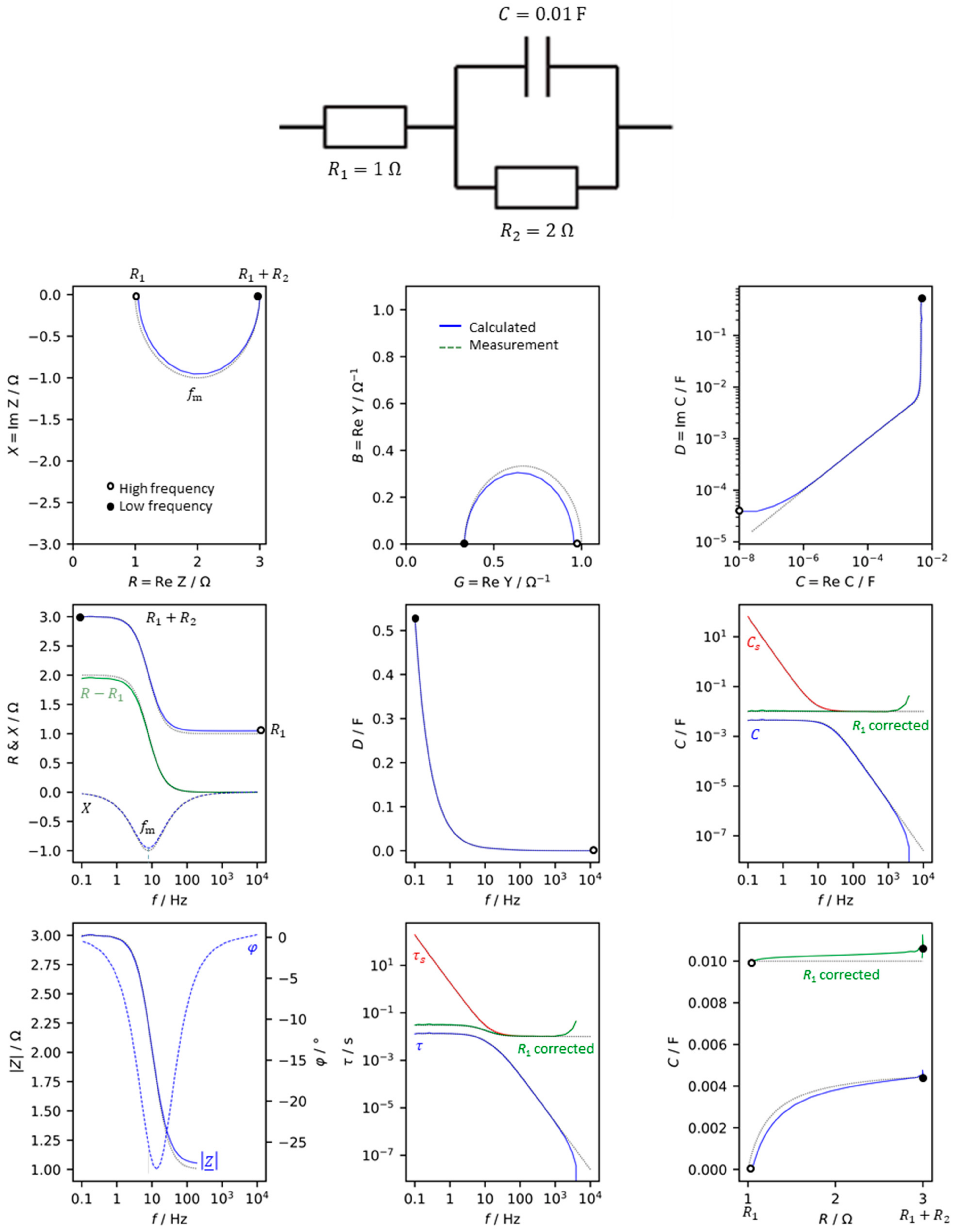
3.1. Simple Equivalent Circuit Diagram

For the simple equivalent circuit diagram of an electrochemical cell (consisting of electrical resistance R₁, polarization resistance R₂, double layer capacitance C), the complex impedance is calculated as in Equation (10).

$$\underset{\_}{Z}\left(\mathrm{j}\mathsf{\omega }\right)=R_1+\frac{1}{\frac{1}{R_2}+\mathrm{j}\omega C}=R_1+\frac{R_2}{1+{\left(\omega R_{2}C\right)}^2}+\mathrm{j}\frac{-\omega R_2^{2}C}{1+{\left(\omega R_{2}C\right)}^2}$$

(10)

The impedance Z = R + jX and the values derived from it are shown in Figure 1. The diagrams are the graphical representations of all the impedance-related quantities for a simple equivalent circuit diagram in the frequency range of 1 mHz to 1 MHz.

• The resistance and reactance describe a semicircle in the complex plane. In the mathematical convention used in electrotechnical engineering, the capacitive values are negative (Im Z < 0) and the inductive behavior is Im Z > 0. In the electrochemical literature, –Im Z is drawn on the ordinate, and the semicircle appears inverted in the so-called Nyquist plot.
• The admittance, the reciprocal of the impedance, Y = 1/Z, shows a semicircle in the complex plane too.
• Complex capacitance C is less meaningful in the complex plane for practical purposes on the frequency scale; pseudocapacitance C(ω), according to Equation (5), reaches the value of the fully charged capacitor C at low frequencies. Above 100 Hz, the capacitance collapses because there is not enough time to charge the capacitor. The imaginary part of the complex capacitance (dissipation D) summarizes the ohmic losses of the network in different frequency regions.

Moreover, Figure 1 compares the simulated values of the network (Equation (10)) with the measurement of a real electrical circuit. Apart from the tolerances of the real components, there are small deviations at high frequencies, which are obvious due to the inductive behavior of the capacitor winding, cables, contacts, and resistive materials. In practice, the capacitance of the electrolytic capacitor used is a frequency-dependent quantity.

If pseudocapacitance C(ω) is corrected by the electrolyte resistance R_e (according to Equation (6)), this ideal capacitance, C = 0.01 F, is received for all frequencies. In contrast to this, series capacitance C_S = −X/ω (which neglects the internal resistance) is valid only for high frequencies. Therefore, C_s should not be used as a measure for the ‘capacitance’.

The time constant can be determined from the frequency at the minimum of the locus curve: τ = ω⁻¹ = R₂C = (2π ⋅ 7.96 Hz)⁻¹ = 0.02 s. Again, the time constant should be calculated from arbitrary measured values over the frequency range using the pseudocapacitance corrected by the electrolyte resistance (Equation (6)). The uncorrected pseudocapacitance is valid only at low frequencies (τ = RC), while C_s is only useful at high frequencies.

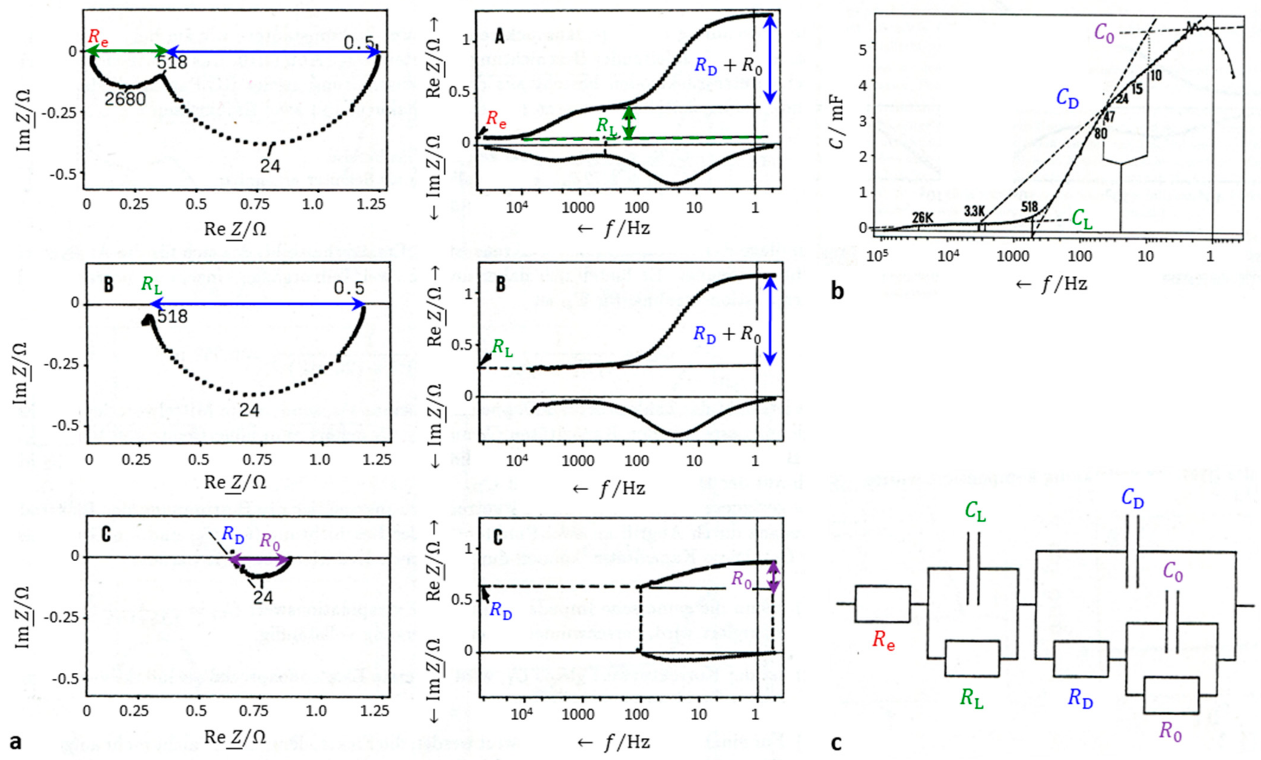
3.2. Stepwise Analysis of Pseudocapacitance

In simple terms, any type of electrochemical cell can be described by an equivalent circuit composed of a series combination of the electrolyte resistance R₁ and the charge transfer impedance R₂||C₂. The latter is essentially the same as the charge transfer resistance R₂ and the double-layer capacitance C₂.

If the electrode processes are more complex than solely determined by charge transfer, the Faraday impedance, which comprises the adsorption, diffusion, and chemical reaction in a transmission line model, can be analyzed by a stepwise procedure [11]. The graphical result of data correction for a technical lead dioxide electrode is shown in Figure 2.

For each semicircle, we proceed as follows.

• Find the electrolyte resistance R₁ = R_e as the intercept of the impedance spectrum with the real axis at high frequencies. Subtract R₁ from all impedance values Z (Figure 2a, top line A). The double-layer capacitance C_L is the extrapolation value of pseudocapacitance C₂ at high frequencies (Figure 2b).

$${\underset{\_}{Z}}_1\left(\mathrm{j}\omega \right)=\underset{\_}{Z}\left(\mathrm{j}\omega \right)-R_1$$

(11)

$$C_2=\underset{\omega \to \infty }{\lim }\frac{-X}{\omega \cdot \left[{\left(R-R_1\right)}^2+X^2\right]}$$

(12)

2.

Correct the double-layer capacitance C₂ in all impedance values to obtain the complex Faraday impedance Z₂. Here, h₁ is an auxiliary variable. The charge transfer resistance R₂ is obtained as the intercept with the real axis at high frequencies (Figure 2a, line C). The pseudocapacitance is corrected by R₂ to give a residual polarization capacitance C_p2, which describes mass transport phenomena.

$$h_1={\left(\mathrm{R}\mathrm{e} {\underset{\_}{Z}}_1\right)}^2+{\left(\mathrm{I}\mathrm{m} {\underset{\_}{Z}}_1\right)}^2$$

(13)

$${\underset{\_}{Z}}_2\left(\mathrm{j}\omega \right)=\frac{\mathrm{R}\mathrm{e} {\underset{\_}{Z}}_1/h_1+\mathrm{j} \left[\mathrm{I}\mathrm{m} {\underset{\_}{Z}}_1/h_1+\omega C_2\right]}{{\left[\mathrm{R}\mathrm{e} {\underset{\_}{Z}}_1/h_1\right]}^2+{\left[\mathrm{I}\mathrm{m} {\underset{\_}{Z}}_1/h_1+\omega C_2\right]}^2}\ge R_2$$

(14)

$$C_{\mathrm{p}2}\left(\omega \right)=\frac{-\mathrm{I}\mathrm{m} {\underset{\_}{Z}}_2}{\omega \left[{\left(\mathrm{R}\mathrm{e} {\underset{\_}{Z}}_2-R_2\right)}^2+{\left(\mathrm{I}\mathrm{m} {\underset{\_}{Z}}_2\right)}^2\right]}\ge C_3$$

(15)

3.

To further analyze the faradaic impedance Z₂, repeat the above calculations in Equations (11)–(15) (replace index 2 with 3 and index 1 with 2). In the first step of the second loop, instead of the electrolyte resistance, the interlayer resistance R_L for the first semicircle is found and subtracted (Figure 2a, line B). In the example, for the semicircle at the highest frequencies, there is no faradaic impedance. However, the second semicircle can be further analyzed to give the charge transfer resistance R_D and the residual polarization resistance R₀ (Figure 2a, line C).

With this, all network elements in the equivalent circuit in Figure 2c have received their values. According to this extrapolation procedure, the impedance spectrum of the PbO₂|Ti electrode in Figure 2c reveals three separate processes: R_e = 0.069 Ω (electrolyte), R_L = 0.29 Ω, C_L = 0.018 mF (interlayer), R_D = 0.60 Ω (charge transfer), C_D = 3.1 mF (double layer), R₀ = 0.24 Ω, C₀ = 4.7 mF (residual faradaic and mass transport impedance).

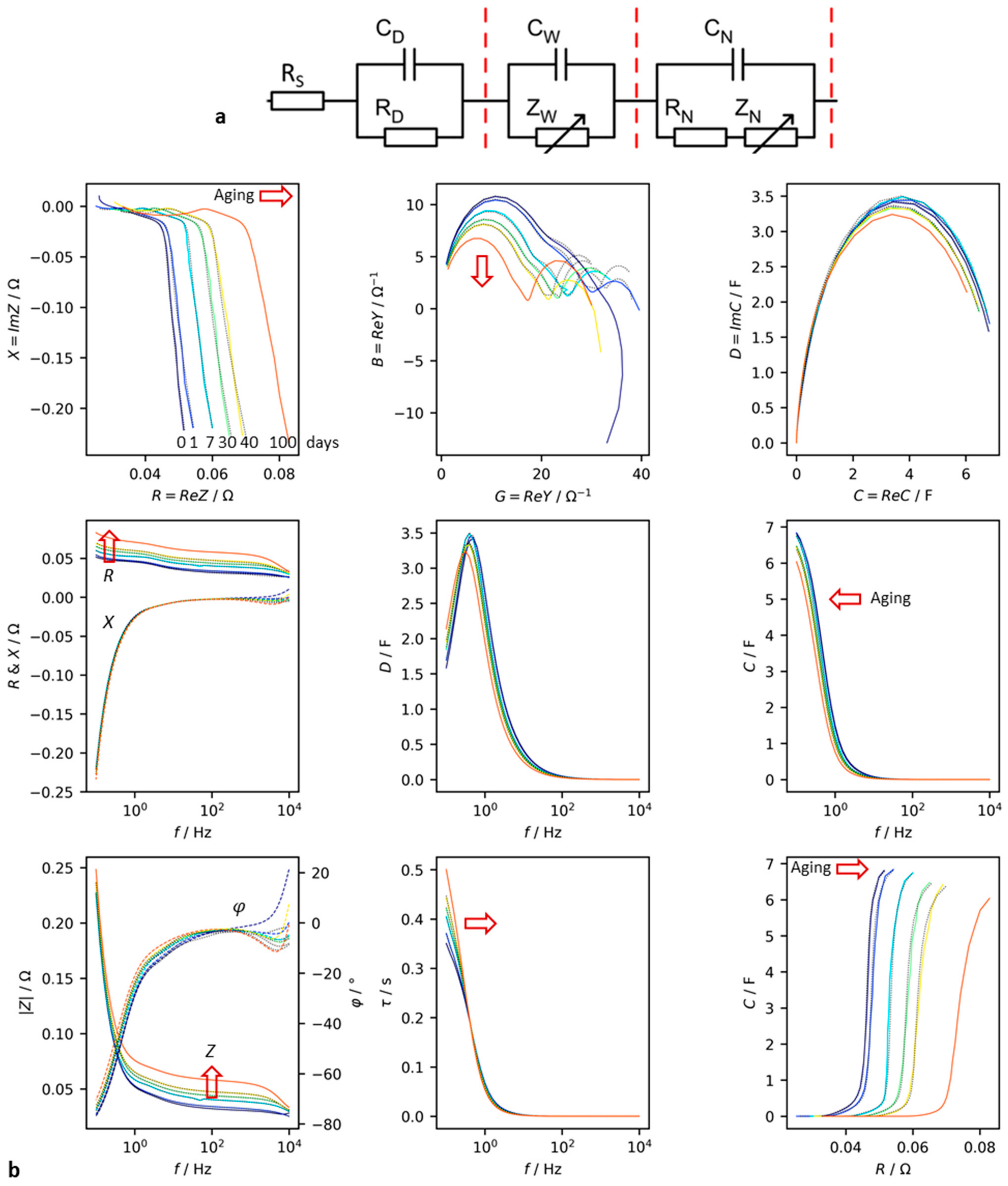
3.3. Aging of Supercapacitors

Figure 3 shows an application example of the aforementioned diagrams for a supercapacitor. Aging under abusive conditions, such as high temperatures and a high voltage, leads to significant changes in the impedance spectra.

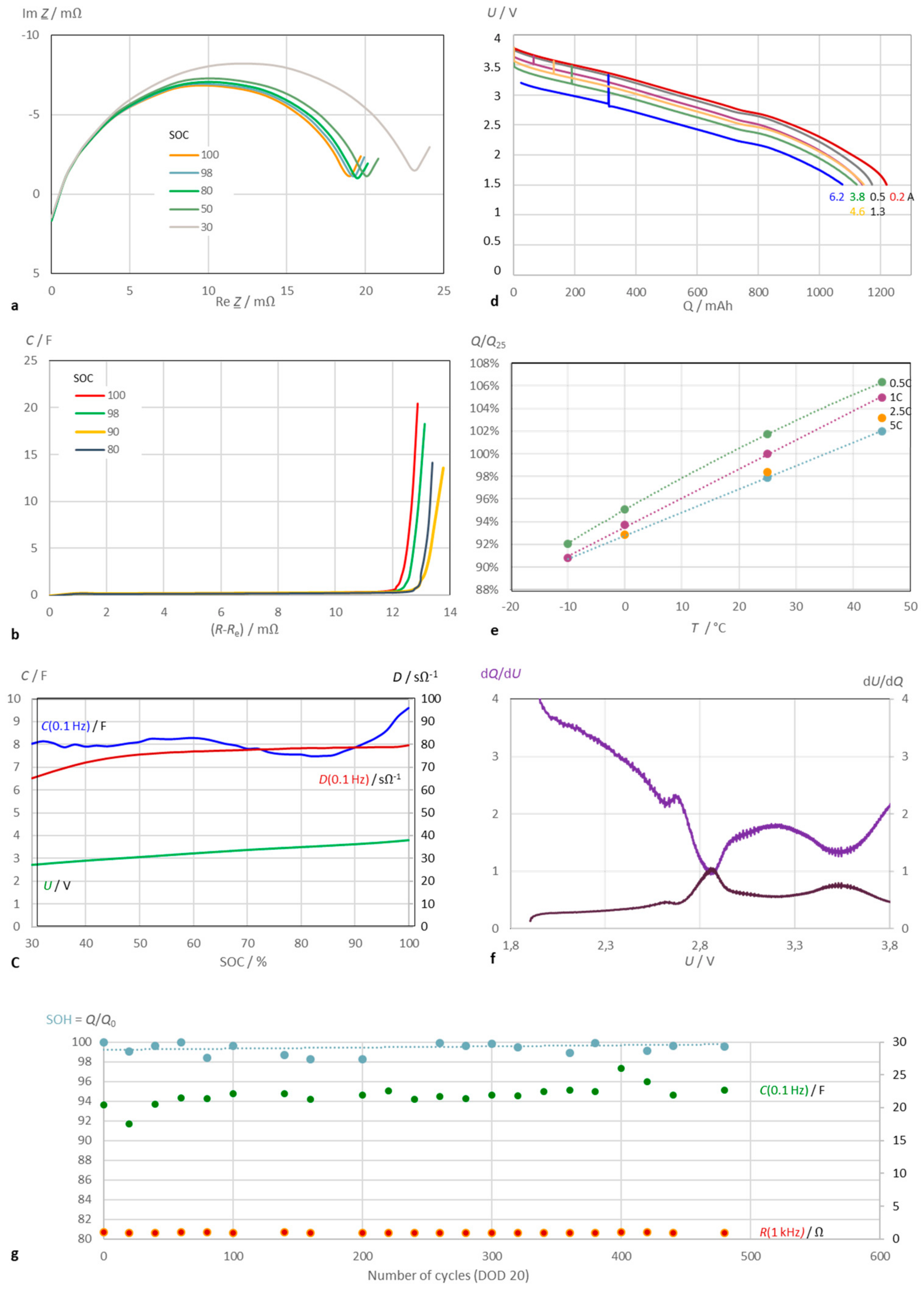
• The impedance in the complex plane mainly shows an increase in internal resistance by shifting the curves towards higher real parts, while the impact of aging on the imaginary parts is less pronounced. This fact is also evident from the frequency response R(ω) and X(ω). The Bode plot illustrates the relationship between the modulus and phase shift.
• The admittance reflects the loss of both conductivity and susceptance during aging.
• The complex capacitance also deteriorates over time. Both pseudocapacitance C and dissipation D decline with time, particularly at frequencies below 10 Hz. The relationship between D and the frequency exhibits a maximum that becomes more apparent over time.
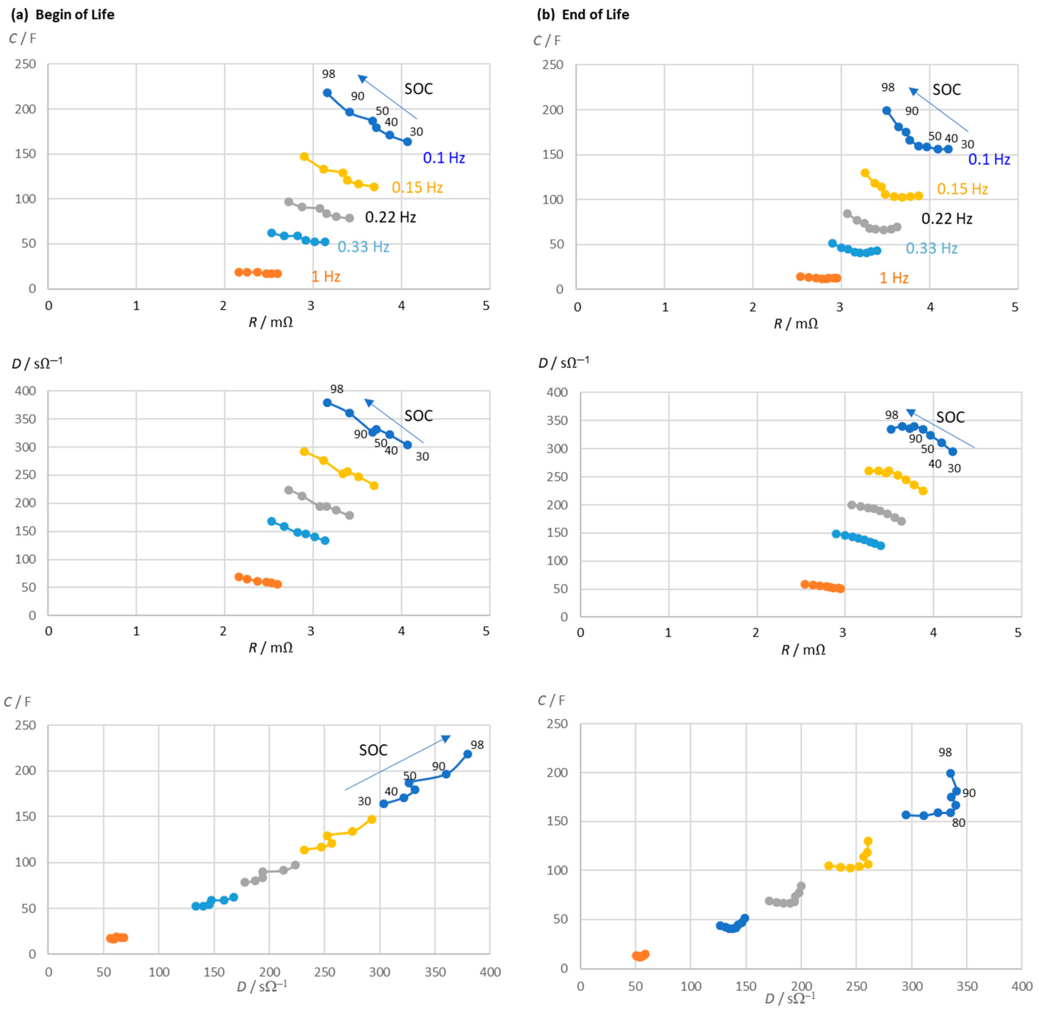
• The capacitance versus resistance diagram provides a clear illustration of the aging process. At high resistance and low capacitance, the left capacitor is the best, while the right one is the worst. The time constant τ = RC increases during aging.

The impedance spectra were fitted to an equivalent circuit network consisting of the electrolyte resistance R_S, double-layer capacitance C_D, charge transfer resistance R_D, a Warburg-like diffusion impedance C_W||Z_W (Equation (16)), and a Nernst-diffusion impedance (Equation (16)).

$$Z_{\mathrm{W}}=\frac{A}{\sqrt{\mathrm{j}\omega }}$$

(16)

$$Z_{\mathrm{N}}=\frac{A_{\mathrm{N}}}{\sqrt{\mathrm{j}\omega }}\tanh \sqrt{\frac{\mathrm{j}\omega }{k_{\mathrm{N}}}}$$

(17)

During the aging process, the electrolyte resistance and charge transfer resistance increase, while the double-layer capacitance drops significantly. However, the diffusion capacitance C_w and diffusion resistance R_N only experience a slight decrease. The capacitance related to the pore structure and ion adsorption (C_N) is halved during the 100-day test.

To quantitatively assess the aging, the charge transfer resistance (from the complex plane plot), electrolyte resistance, and pseudocapacitance from the C(R) plot can be easily evaluated. This empirical evaluation of the impedance spectra avoids the need for cumbersome and arbitrary equivalent circuit models. Curve fitting to equivalent circuits often does not adequately reflect the electrochemical reality and is prone to numerical errors.

4. Battery State Indicators and Cell Diagnosis

4.1. Correlation of Electric Charge and Impedance

The state of charge (SOC = Q/Q_N) [23,24] describes the relationship between the currently available electric charge (capacity) and the rated capacity Q_N of the new battery. SOC = 100% represents the full charge, and SOC = 0 is the empty battery.

Since the 1930s, voltage measurements [25,26,27,28] have been used to determine the SOC [29,30,31], but they do not work well with flat voltage curves like those of the LiFePO₄ system. Moreover, lithium-ion batteries are not supposed to be discharged below a certain voltage (the cut-off voltage).

Impedance spectroscopy [32,33,34,35,36], Coulomb counting, bookkeeping methods, and look-up tables have been used since the mid-1970s. Unfortunately, the impedance method does not deliver Ah capacities because pseudocapacitance is a differential quantity.

$$C=\frac{\mathrm{d}Q}{\mathrm{d}U} \Rightarrow Q=\underset{0}{\overset{\mathsf{\Delta }U}{\int }}C\left(U\right) \mathrm{d}U$$

(18)

The actual cell voltage is U(t) at time t after starting the impedance measurement. The frequency-dependent pseudocharge Q(ω,t) is only a qualitative measure for the instantaneous electrical charge because there is a numerical factor connecting true battery capacity Q [37] and pseudocharge.

4.2. Failure Analysis Using Impedance Spectroscopy

The state of health (SOH = Q₀/Q_N) describes how much of its initial capacity a battery has left after it has been used for a while. It compares the capacity of a fully charged, old battery (Q₀) to the rated or nominal capacity of a new battery (Q_N). There is still no simple method to determine the charge of a battery that can be used without completely discharging it.

Impedance spectroscopy shows all the changes in a battery’s resistance and capacitance during normal use and in cases of misuse [38]: lithium plating, short circuits, overcharge, deep discharge, phase changes, and thermal runaway.

The degradation of a Li-ion cell depends on how the cell is used during its lifetime and stressed by extrinsic factors (time, temperature, SoC level, C rate, DoD, mechanical stress) [39].

There is no clear consensus in the literature as to whether it is better to use the resistance or reactance to estimate the battery life.

• It is worth noting that the electrolyte resistance measured at high frequencies (above 1 kHz) does not decrease in a strictly linear way with a rising temperature. If there are any internal short circuits caused by mechanical deformations, a drop in ohmic resistance occurs at frequencies above 100 Hz [40]. R_e can be used a measure for the SOH [41].
• The ohmic resistance at medium frequencies—for instance, R(1 Hz) or R (0.1 Hz)—is often correlated with the battery capacity and the SOH [42,43,44]. However, the resistance reflects the growth of the passive layer (SEI) and the decomposition of the electrolyte, rather than the actual available capacity. In the complex plane, one or two depressed semicircles are visible (see Section 3.2). The low-frequency region (<0.1 Hz), which represents the diffusion processes at the two electrodes, is often neglected because of the longer time required to measure the impedance at low frequencies.
• The pseudocapacitance reflects the storage properties of the cell, whereas the resistance shows the kinetic inhibitions. In a C(R) plot, the healthiest operating state is characterized by the curve at the lowest resistance and highest capacitance (Kurzweil [1,12]).
• The phase shift [45] rises quite suddenly shortly before cell venting (within seconds) and thermal runaway (some minutes later), although the cell voltage remains constant [46].

4.3. Correlation of Impedance and Current/Voltage Characteristics

Electrochemical cells exhibit more or less non-linear current/voltage characteristics. Therefore, the real part of the impedance at low frequencies, which is the approximate DC resistance R, reflects the slope (tangent) of the current/voltage characteristics at the given stationary operating point of the cell.

$$R\left(\omega \to 0\right)=\frac{\mathrm{d}U}{\mathrm{d}I}\approx \frac{U}{I}$$

(19)

Pseudocapacitance C, determined by impedance spectroscopy, reflects the slope of the charge/voltage curve, which represents the approximate ratio of the capacity change to the voltage change. It is found that, at the same voltage, the differential capacity dQ/dU from the charge/discharge curves and the pseudocapacitance at low frequencies from the impedance spectra are more or less the same [47]. To avoid any problems with the numerical calculation, it is best to calculate the dQ/dU (capacitance) from the charge/discharge curves as the reciprocal of the differential voltage [48]. Equation (20) gives an indication of how the capacitance and resistance change as the state of charge changes.

$$C(\omega \to 0)=\frac{\mathrm{d}Q}{\mathrm{d}U}={\left(\frac{\mathrm{d}U}{\mathrm{d}\mathrm{Q}}\right)}^{-1}={\left(\frac{\mathrm{d}R}{\mathrm{d}t}\right)}^{-1}$$

(20)

dQ/dU is measured in Farads. F = C/V = As V⁻¹. Thus, it is important not to confuse the symbol for electrical capacitance, C, with the meaning and symbol for the electrical charge (capacity Q).

The term ‘differential capacity analysis’ first appeared around 2000. It refers to the first derivative of the galvanostatic curve, U(Q). However, it is difficult to quantitatively compare C(ω) from impedance measurements with the ‘incremental capacity’ dQ/dU and its reciprocal dU/dQ, described by Bloom [49], Dubarry [50], Dahn [51], and Smith [52]. Unfortunately, the noisy differential curves require the previous smoothing of the data.

The different cell chemistries of lithium-ion batteries show similar results, even though the available charge and state of charge (SOC) do not change in a linear way with the voltage. It is not always clear that the SOC and SOH are related to the differential capacity.

dQ/dU from the constant/current (chronopotentiometric) curves yields the following information [46]:

• Differential capacity dQ/dU peaks appear at regions where the U(Q) curve is flat, when the battery reaches a phase equilibrium of coexisting phases with different lithium concentrations (ΔU→0) and the cell voltage is constant (Bloom [47]).
• The peaks in dU/dQ reflect phase transitions and characterize the ‘almost empty’ or ‘almost full’ battery, when a constant current can no longer be fed into or drawn from it (ΔI→0). If the ‘differential voltage’ rises quickly, it means that the battery has been overcharged or deeply discharged. In this case, the differential capacity is small. The distance between two inflection points on the differential voltage curve is proportional to the battery capacity, which can be used to estimate the battery SOH [53].
• In the case of depletion or overcharge, capacitance C (slope of the Q(U) curve) is small and resistance R (slope of the U(Q) curve) is great. dQ/dU and dU/dQ intersect at a point below the upper limit voltage, which is located at the kink point near the full charge [48].

5. Application Example: Lithium-Ion Battery

Which quantity derived from the impedance spectra best indicates the state of charge of a battery?

Figure 4 shows the aging of a lithium-ion battery. Comparing the resistance, reactance, and capacitance at a fixed frequency of 0.1 Hz, it can be seen that the internal resistance of the battery (the real part of the impedance) increases linearly with increasing aging. In this example, the electrolyte correction, R (0.1 Hz) − R_e, brings little improvement for the linearity (Figure 4a) but is useful for the capacitance (Figure 4c).

The imaginary part of the impedance and the phase shift do not correlate strictly with the state of charge (Figure 4b). The best full charge indication is the pseudocapacitance C (0.1 Hz) corrected by the electrolyte resistance (Figure 4e). This is intuitively understood from the correlation between the available charge and capacitance (Q = CU). The series capacitance C_S according to the approximation in Equation (6) is of little use. Additionally, the correlation between the SOH and impedance modulus, dissipation, and time constant is poor.

Figure 5 shows the resistance and capacitance of a lithium-ion battery during a cycle life test. The lower the frequency of the excitation signal, the clearer the approximately linear relationship between the capacitance and SOC. C(0.1 Hz) takes longer to measure than C (0.33 Hz), which works equally well. Dielectric losses can also be used, but capacitance C retains its relationship with the SOC better than dissipation D over the life of the battery.

The quotient of the pseudocapacitance and dissipation reflects the ratio of the reactance and resistance (at frequency ω). Both quantities are inextricably linked to the SOC. When calculating C and D, it is advisable to correct for the electrolyte resistance to improve the charge indication.

$$\frac{C\left(\omega \right)}{D\left(\omega \right)}=-\frac{X\left(\omega \right)}{R\left(\omega \right)}$$

(21)

6. Application Example: Sodium-Ion Battery

Figure 6 presents a comprehensive overview of the diagrams and calculation methods described, using the example of a sodium-ion battery with a capacity of 1.1 Ah. The new battery was initially characterized using impedance spectroscopy.

During discharge, the diameters of the locus curve arcs increase, while the pseudocapacitance decreases (Figure 6a,c). The dissipation D is calculated as the imaginary part of the complex capacitance and indicates best the state of charge at a low SOC (Figure 6c), while the pseudocapacitance C increases linearly at full charge (SOC > 85%). However, the linearity of C(SOC) is worse than with lithium-ion batteries.

The battery capacity Q was determined by constant current discharge (Ah counting) and is dependent on both the temperature and load current (Figure 6d,e). The discharge curve allows us to calculate the differential capacity (incremental capacity, dQ/dU) and incremental voltage (dU/dQ), which are equal at an approximately 2.8 V cell voltage (Figure 6f). At this voltage, the discharge curve exhibits a local plateau before the battery is fully discharged and exhausted.

The sodium-ion battery exhibits good stability over several hundred charge/discharge cycles (from SOC 100% to 80%). The nearly constant electrical charge (battery capacity) correlates with the pseudocapacitance and polarization resistance. After 3600 cycles, the capacity drops to SOH = 98%, as shown in Figure 6g.

7. Discussion

Prior state-of-the-art methods for SOC monitoring require ampere-hour counting during a complete discharge. The cell voltage is a less accurate method of measuring the actual electric charge. There is a clear correlation between the pseudocapacitance and the remaining capacity for the main types of lithium-ion batteries.

7.1. Evaluation of Impedance Spectra without Model Assumptions

The commonly used adaptation of complex plane curves to electrotechnical equivalent circuit diagrams is unsuitable if the electrochemistry changes due to aging processes. Additionally, there is no guarantee that the selected equivalent circuit diagram will accurately represent the electrode processes and continue to do so in the future. Therefore, it is advisable to evaluate the impedance spectrum without a predefined model by subtracting the electrolyte resistance and the double-layer capacitance step by step and further decomposing the remaining pseudocapacitance (refer to Section 3.2).

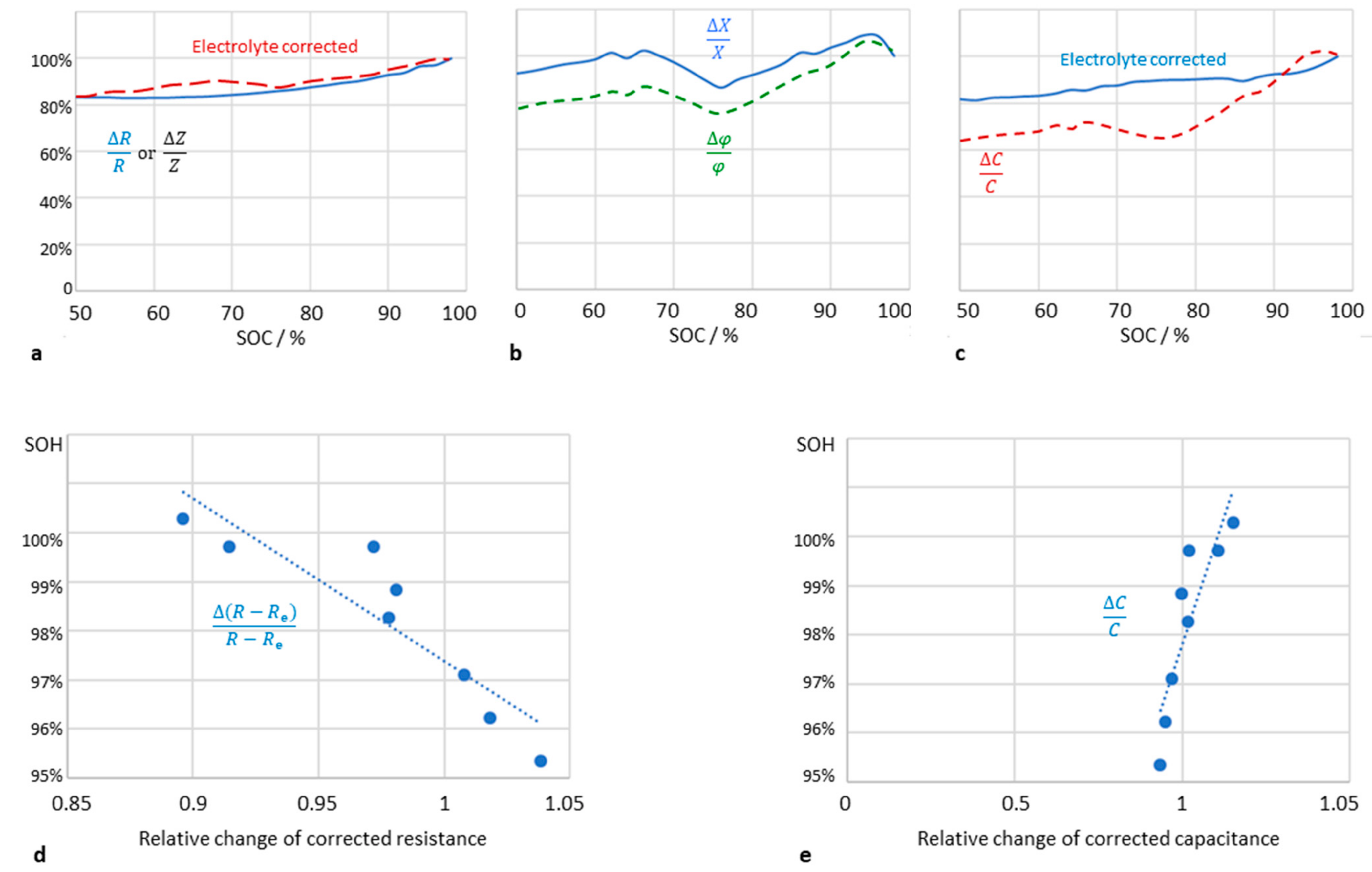
7.2. SOC and SOH Monitoring

The prediction of the state of charge (SOC) and state of health (SOH) requires a quantity that can linearly map the charge state over a large measuring range. It is worth noting that the Nyquist plot can take different forms even for the same battery chemistry. This raises the question of which physical variable can be meaningfully evaluated for SOC monitoring. Both the real and imaginary parts of the impedance are affected by the state of charge, with the resistance dropping and the capacitance increasing as the SOC increases.

The pseudocapacitance and SOC show their best linear correlation at frequencies below 1 Hz. A quadratic model is also possible: SOC = aC² + bC + c. The predicted SOC values help us to determine whether a battery of the same type and manufacturer is empty, a quarter full, half full, three quarters full, or completely full.

The capacitance does not necessarily have to be measured down to extremely low frequencies. C (0.1 Hz) encompasses the mass-transport-limited charge transfer reaction that is implicated in the lithium-ion intercalation at very low frequencies. The linear trend demonstrates enhanced performance when the SOC range is considered up to 98% (as opposed to 100%), given that overcharge phenomena are observed at full charge.

The electrolyte resistance is not recommended for the determination of the SOC, but it is useful as an aging indicator for SOH monitoring. Therefore, the measured real parts are corrected by subtracting R_e (the real part at a high frequency, where X = 0). The linear trend between the pseudocapacitance and electric charge is better when the electrolyte resistance is corrected.

Overcharging complicates the relationship between the capacitance and state of charge (SOC). The sudden jump in capacitance at SOC = 1 could be used to show that the battery is fully charged, which would avoid the risk of overcharging.

7.3. Correlation of Pseudocapacitance and Battery Capacity

The capacity of a battery, measured as the stored residual electric charge Q, is expected to correlate with the pseudocapacitance (differential capacitance), defined as C = dQ/dU.

Unfortunately, there is no direct quantitative relation between the pseudocapacitance and electric charge. The pseudocapacitance C(ω) is a useful three-in-one quantity that combines information about the resistance, reactance, and frequency.

7.4. Impact of Aging

As a lithium-ion battery ages, its internal resistance increases. The electrolyte resistance is not a good indicator of the battery’s overall condition. As SEI formation progresses, the electrolyte resistance increases until two arcs appear in the impedance spectrum (see Figure 7). Sometimes, new batteries show an apparent improvement in resistance for the first hundred cycles (due to SEI formation), before the undesirable aging processes begin.

The pseudocapacitance can give a good insight into how healthy a battery is, even if the shape of the impedance spectrum changes considerably during the aging process. For combined SOC and SOH measurements, the pseudocapacitance is still a good option. It is beneficial to normalize C(ω) to the fully charged battery (SOC = 1) or the new battery (SOH = 1).

7.5. Impact of Cell Chemistry

The impedance spectra (Figure 7) show three regions that are affected by aging:

• At high frequencies—electrolyte and solid/electrolyte interface (SEI);
• At medium frequencies—charge transfer reaction;
• At low frequencies—pore diffusion and ion intercalation into the host lattice.

Depending on the cell chemistry, the resistance in the three regions increases due to electrolyte decomposition, SEI growth, slowed charge transfer, and related aging effects (lithium dendrite formation, the loss of anode materials, particle cracking on the cathode). Electrolyte decomposition can be associated with a shift to higher ohmic resistance. Anode degradation and SEI layer growth increase the first quarter circle in the mid-frequency region. The formation of a cathode electrolyte interface (CEI) and cathode particle cracking shift the second arc. An increase in the low-frequency region shows cathode structural disordering (Jurilli [39]).

It is beneficial to remove the electrolyte resistance (where it meets the real axis) to create a set of curves that are independent of contact and cable errors. This also excludes the corrosion resistance of the current collectors. Once the real part has been corrected, the modulus of the impedance, |Z(ω)|, and the pseudocapacitance, C(ω) = −Im Z/(ω |Z|²), can be calculated. The shape of the diffusion impedance at low frequencies depends on whether the lithium-ions are mobile in linear channels (Li_1−xFePO₄), in areas of the layer lattice (Li_1−xCoO₂, NMC), or in the void spaces of a spinel (Li_1−xMn₂O₄, LMO).

We need to conduct more research to improve the impedance method so that we can manage the steps in the voltage/capacity curve and overcharging effects properly.

8. Conclusions

The theory, principles, equipment, and interpretation of impedance measurements in various applications have been extensively described in the literature, e.g., the highly useful tutorial in [54]. This paper shows the practical applications of impedance spectroscopy and the graphical interpretation of the measured data without the need for complex numerical tools and arbitrary methods to fit the values to non-linear models.

It has been shown which quantities can be derived in principle from the complex impedance Z and how to calculate them. The most useful quantities are ohmic resistance R, reactance X, and pseudocapacitance C, which can be plotted on the complex plane or on a frequency scale. The importance and usefulness of the frequency response of pseudocapacitance has been clarified with regard to the empirical evaluation of impedance spectra. Less useful for electrochemical interpretation, or limited to specific problems, are the impedance modulus |Z|, the phase shift φ, the dissipation D (the imaginary part of the complex capacitance), and the time constant τ. The mathematical sign convention (capacitive = negative reactance) is recommended to avoid inconsistencies in all cases where different impedance-derived quantities are used.

Impedance spectroscopy can be used to monitor the aging behavior of electrochemical cells such as batteries, supercapacitors, and electrodes in electrolysis. In particular, the pseudocapacitance versus resistance plot (see, for example, Figure 3) helps to determine whether aging processes are driven more by an increase in resistance (as a measure of power loss and growing interlayers) or a gradual decrease in pseudocapacitance (as a measure of the active surface area and electric charge).

The correction procedure (presented in Section 3.2) allows a stepwise analysis of the semicircles in the complex plane with respect to the electrolyte resistance and the equivalent resistances and capacitances of the faradaic and non-faradaic electrode reactions.

Unlike ampere-hour counting during a full discharge, the impedance method is fast but does not give quantitative results for the SOC and SOH. Each cell chemistry has its own conversion factor between the pseudocapacitance and ‘true’ electrical charge. If the discharge curve has steps, the clear linear relationship C(SOC) is often lost. In essence, semi-quantitative SOC and SOH values can be determined by means of calibration curves [1].

Impedance spectroscopy is undoubtedly a superior tool for the analysis of time-varying and changing electrochemical cells, because it allows a direct, visual interpretation with resistances and capacitances, which is superior to the use of overpotentials and IR drops from current/voltage curves. Beyond the applications shown, impedance spectroscopy opens up the exciting world of capacitive energy storage ceramics [55], bio-electrochemical sensors, and photoelectrochemical cells.

References

1. Kurzweil, P.; Scheuerpflug, W. State-of-Charge Monitoring and Battery Diagnosis of Different Lithium Ion Chemistries Using Impedance Spectroscopy. Batteries 2021, 7, 17. [Google Scholar] [CrossRef]
2. Kurzweil, P.; Schottenbauer, J.; Schell, C. Past, Present and Future of Electrochemical Capacitors: Pseudocapacitance, Aging Mechanisms and Service Life Estimation. J. Energy Storage 2021, 35, 102311. [Google Scholar] [CrossRef]
3. Trasatti, S.; Kurzweil, P. Electrochemical Supercapacitors as Versatile Energy Stores. Platin. Met. Rev. 1994, 38, 46–56. [Google Scholar] [CrossRef]
4. Kurzweil, P.; Scheuerpflug, W.; Frenzel, B.; Schell, C.; Schottenbauer, J. Differential Capacity as a Tool for SOC and SOH Estimation of Lithium Ion Batteries Using Charge/Discharge Curves, Cyclic Voltammetry, Impedance Spectroscopy, and Heat Events: A Tutorial. Energies 2022, 15, 4520. [Google Scholar] [CrossRef]
5. Bard, A.J.; Faulkner, L.R.; White, H.S. Electrochemical Methods: Fundamentals and Applications, 3rd ed.; J. Wiley: Hoboken, NJ, USA, 2022. [Google Scholar]
6. Barsoukov, E.; Macdonald, J.R. Impedance Spectroscopy: Theory, Experiment, and Applications, 3rd ed.; J. Wiley: Hoboken, NJ, USA, 2018. [Google Scholar]
7. Gabrielli, C. Identification of Electrochemical Processes by Frequency Respsonse Anaylsius; Solatron Group: Farnborough, UK, 1980. [Google Scholar]
8. Huang, J.; Li, Z.; Liaw, B.Y.; Zhang, J. Graphical analysis of electrochemical impedance spectroscopy data in Bode and Nyquist representations. J. Power Sources 2016, 309, 82–98. [Google Scholar] [CrossRef]
9. Nyquist, H. Regeneration theory. Bell Syst. Tech. J. 1932, 11, 126–147. [Google Scholar] [CrossRef]
10. Cole, K.; Cole, R. Dispersion and adsorption in dielectrics. I. alternating current characteristics. J. Chem. Phys. 1941, 9, 341–351. [Google Scholar] [CrossRef]
11. Kurzweil, P.; Ober, J.; Wabner, D.W. Method for extracting kinetic parameters from measured impedance spectra. Electrochim. Acta 1989, 34, 1179–1185. [Google Scholar] [CrossRef]
12. Kurzweil, P.; Fischle, H.J. A new monitoring method for electrochemical aggregates by impedance spectroscopy. J. Power Sources 2004, 127, 331–340. [Google Scholar] [CrossRef]
13. Mansfeld, F.; Kendig, M.W.; Tsai, S. Evaluation of Corrosion Behavior of Coated Metals with AC Impedance Measurements. Corrosion 1982, 38, 478–485. [Google Scholar] [CrossRef]
14. Macdonald, D.D.; Urquidi-Macdonald, M. Application of Kramers-Kronig Transforms in the Analysis of Electrochemical Systems: I. Polarization Resistance. J. Electrochem. Soc. 1985, 132, 2316–2319. [Google Scholar] [CrossRef]
15. Kramers, H.A. Die Dispersion und Absorption von Röntgenstrahlen. Phys. Z 1929, 30, 522–523. [Google Scholar]
16. Randles, J.E.B. Kinetics of rapid electrode reactions. Discuss. Faraday Soc. 1947, 1, 11–19. [Google Scholar] [CrossRef]
17. Thirsk, H.R.; Armstrong, R.D.; Bell, M.F.; Metcalfe, A.A. Electrochemistry; Thirsk, H.R., Ed.; The Royal Society of Chemistry: London, UK, 1978; Volume 6, pp. 98–127. [Google Scholar]
18. Kronig, R.D.L. On the theory of dispersion of x-rays. JOSA 1926, 12, 547–557. [Google Scholar] [CrossRef]
19. Van Meirhaeghe, R.L.; Dutoit, E.C.; Cardon, F.; Gomes, W.P. On the application of the kramers-kronig relations to problems concerning the frequency dependence of electrode impedance. Electrochim. Acta 1976, 21, 39–43. [Google Scholar] [CrossRef]
20. Walter, G.W. A review of impedance plot methods used for corrosion performance analysis of painted metals. Corros. Sci. 1986, 26, 681–703. [Google Scholar] [CrossRef]
21. Debye, P. Einige Resultate einer kinertischen Theorie der Isolatoren. Phys. Z 1912, 12, 97–100. [Google Scholar]
22. Hahn, M.; Schindler, S.; Triebs, L.C.; Danzer, M.A. Optimized Process Parameters for a Reproducible Distribution of Relaxation Times Analysis of Electrochemical Systems. Batteries 2019, 5, 43. [Google Scholar] [CrossRef]
23. Kurzweil, P.; Shamonin, M. State-of-Charge Monitoring by Impedance Spectroscopy during Long-Term Self-Discharge of Supercapacitors and Lithium-Ion Batteries. Batteries 2018, 4, 35. [Google Scholar] [CrossRef]
24. Waag, W.; Sauer, D.U. State-of-Charge/Health. In Encyclopedia of Electrochemical Power Sources; Dyer, J.C.C., Moseley, P., Ogumi, Z., Rand, D., Scrosati, B., Eds.; Elsevier: Amsterdam, The Netherlands, 2009; Volume 4, pp. 793–804. [Google Scholar]
25. Finger, E.P.; Sands, E.A. Method and Apparatus for Measuring the State of Charge of a Battery by Monitoring Reductions in Voltage. US Patent 4193026A, 11 March 1980. [Google Scholar]
26. Kikuoka, T.; Yamamoto, H.; Sasaki, N.; Wakui, K.; Murakami, K.; Ohnishi, K.; Kawamura, G.; Noguchi, H.; Ukigaya, F. System for Measuring State of Charge of Storage Battery. US Patent 4377787A, 22 March 1983. [Google Scholar]
27. Seyfang, G.R. Battery State of Charge Indicator. US Patent 4,949,046, 14 August 1990. [Google Scholar]
28. Peled, E.; Yamin, H.; Reshef, I.; Kelrich, D.; Rozen, S. Method and Apparatus for Determining the State-of-Charge of Batteries Particularly Lithium Batteries. US Patent 4,725,784 A, 16 February 1988. [Google Scholar]
29. Piller, S.; Perrin, M.; Jossen, A. Methods for state-of-charge determination and their applications. J. Power Sources 2001, 96, 113–120. [Google Scholar] [CrossRef]
30. Gauthier, R.; Luscombe, A.; Bond, T.; Bauer, M.; Johnson, M.; Harlow, J.; Louli, A.J.; Dahn, J.R. How do Depth of Discharge, C-rate and Calendar Age Affect Capacity Retention, Impedance Growth, the Electrodes, and the Electrolyte in Li-Ion Cells? J. Electrochem. Soc. 2022, 169, 020518. [Google Scholar] [CrossRef]
31. Bergveld, J.J.; Danilov, D.; Notten, P.H.L.; Pop, V.; Regtien, P.P.L. Adaptive State-of-charge determination. In Encyclopedia of Electrochemical Power Sources; Dyer, J.C.C., Moseley, P., Ogumi, Z., Rand, D., Scrosati, B., Eds.; Elsevier: Amsterdam, The Netherlands, 2009; Volume 1, pp. 450–477. [Google Scholar]
32. Rodrigues, S.; Munichandraiah, N.; Shukla, A.K. A review of state-of-charge indication of batteries by means of a.c. impedance measurements. J. Power Sources 2000, 87, 12–20. [Google Scholar] [CrossRef]
33. Osaka, T.; Mukoyama, D.; Nara, H. Review—Development of Diagnostic Process for Commercially Available Batteries, Especially Lithium Ion Battery, by Electrochemical Impedance Spectroscopy. J. Electrochem. Soc. 2015, 162, A2529. [Google Scholar] [CrossRef]
34. La Rue, A.; Weddle, P.J.; Ma, M.; Hendricks, C.; Kee, R.J.; Vincent, T.L. State-of-Charge Estimation of LiFePO4–Li4Ti5O12 Batteries using History-Dependent Complex-Impedance. J. Electrochem. Soc. 2019, 166, A404. [Google Scholar]
35. Huang, J.; Gao, Y.; Luo, J.; Wang, S.; Li, C.; Chen, S.; Zhang, J. Impedance Response of Porous Electrodes: Theoretical Framework, Physical Models and Applications. J. Electrochem. Soc. 2020, 167, 166503. [Google Scholar] [CrossRef]
36. Wang, X.; Wei, X.; Zhu, J.; Dai, H.; Zheng, Y.; Xu, X.; Chen, Q. A review of modeling, acquisition, and application of lithium-ion battery impedance for onboard battery management. eTransportation 2021, 7, 100093. [Google Scholar] [CrossRef]
37. Wenzl, H. Capacity. In Encyclopedia of Electrochemical Power Sources; Dyer, J.C.C., Moseley, P., Ogumi, Z., Rand, D., Scrosati, B., Eds.; Elsevier: Amsterdam, The Netherlands, 2009; Volume 1, pp. 395–400. [Google Scholar]
38. Hung, M.H.; Lin, C.H.; Lee, L.C.; Wang, C.M. State-of-charge and state-of-health estimation for lithium-ion batteries based on dynamic impedance technique. J. Power Sources 2014, 268, 861–873. [Google Scholar] [CrossRef]
39. Iurilli, P.; Brivio, C.; Wood, V. On the use of electrochemical impedance spectroscopy to characterize and model the aging phenomena of lithium-ion batteries: A critical review. J. Power Sources 2021, 505, 229860. [Google Scholar] [CrossRef]
40. Spielbauer, M.; Berg, P.; Ringat, M.; Bohlen, O.; Jossen, A. Experimental study of the impedance behavior of 18650 lithium-ion battery cells under deforming mechanical abuse. J. Energy Storage 2019, 26, 101039. [Google Scholar] [CrossRef]
41. Choi, W.; Shin, H.C.; Kim, J.M.; Choi, J.Y.; Yoon, W.S. Modeling and applications of electrochemical impedance spectroscopy (EIS) for lithium-ion batteries. J. Electrochem. Sci. Technol. 2002, 11, 1–13. [Google Scholar] [CrossRef]
42. Eddahech, A.; Briat, O.; Woirgard, E.; Vinassa, J.M. Remaining useful life prediction of lithium batteries in calendar ageing for automotive applications. Microelectron. Reliab. 2012, 52, 2438–2442. [Google Scholar] [CrossRef]
43. Galeotti, M.; Cinà, L.; Giammanco, C.; Cordiner, S.; Di Carlo, A. Performance analysis and SOH (state of health) evaluation of lithium polymer batteries through electrochemical impedance spectroscopy. Energy 2015, 89, 678–686. [Google Scholar] [CrossRef]
44. Howey, D.A.; Mitcheson, P.D.; Yufit, V.; Offer, G.J.; Brandon, N.P. Online Measurement of Battery Impedance Using Motor Controller Excitation. IEEE Trans. Veh. Technol. 2014, 63, 2557–2566. [Google Scholar] [CrossRef]
45. Dowgiallo, E.J. Method for Determining Battery State of Charge by Measuring A.C. Electrical Phase Angle Change. US Patent 3984762A, 5 October 1976. [Google Scholar]
46. Srinivasan, R.; Demirev, P.A.; Carkhuff, B.G. Rapid monitoring of impedance phase shifts in lithium-ion batteries for hazard prevention. J. Power Sources 2018, 405, 30–36. [Google Scholar] [CrossRef]
47. Guo, D.; Yang, G.; Zhao, G.; Yi, M.; Feng, X.; Han, X.; Lu, L.; Ouyang, M. Determination of the Differential Capacity of Lithium-Ion Batteries by the Deconvolution of Electrochemical Impedance Spectra. Energies 2020, 13, 915. [Google Scholar] [CrossRef]
48. Kurzweil, P.; Frenzel, B.; Scheuerpflug, W. A novel evaluation criterion for the rapid estimation of the overcharge and deep discharge of lithium-ion batteries using differential capacity. Batteries 2022, 8, 86. [Google Scholar] [CrossRef]
49. Bloom, I.; Christophersen, J.; Gering, K. Differential voltage analyses of high-power lithium-ion cells, 2. Applications. J. Power Sources 2005, 139, 304–313. [Google Scholar] [CrossRef]
50. Dubarry, M.; Svoboda, V.; Hwu, R.; Liaw, B.Y. Incremental capacity analysis and close-to-equilibrium OCV measurements to quantify capacity fade in commercial rechargeable lithium batteries. Electrochem. Solid State Lett. 2006, 9, A454. [Google Scholar] [CrossRef]
51. Dahn, H.M.; Smith, A.J.; Burns, J.C.; Stevens, D.A.; Dahn, J.R. User-Friendly Differential Voltage Analysis Freeware for the Analysis of Degradation Mechanisms in Li-Ion Batteries. J. Electrochem. Soc. 2012, 159, A1405. [Google Scholar] [CrossRef]
52. Smith, A.J.; Dahn, J.R. Delta Differential Capacity Analysis. J. Electrochem. Soc. 2012, 159, A290. [Google Scholar] [CrossRef]
53. Wang, L.; Zhao, X.; Liu, L.; Pan, C. State of health estimation of battery modules via differential voltage analysis with local data symmetry method. Electrochim. Acta 2017, 256, 81–89. [Google Scholar] [CrossRef]
54. Lazanas, A.C.; Prodromidis, M.I. Electrochemical Impedance Spectroscopy—A Tutorial. ACS Meas. Sci. Au 2023, 3, 162–193. [Google Scholar] [CrossRef] [PubMed]
55. Zhang, L.; Pu, Y.; Chen, M. Complex impedance spectroscopy for capacitive energy-storage ceramics: A review and prospects. Mater. Today Chem. 2023, 28, 101353. [Google Scholar] [CrossRef]
Figure 1. Basic graphical representations of impedance-related quantities for a simple equivalent circuit diagram in the frequency range of 1 mHz to 1 MHz. Mathematical convention. R = resistance, X = reactance, G = conductance, B = susceptance, C = capacitance, D = dissipation, |Z| = impedance modulus, φ = phase shift between voltage and current, τ = time constant. Solid lines (–): measured values for an electric circuit with real resistors and capacitor. Dotted (······): calculated values for the ideal network.
Batteries 10 00177 g001
Figure 2. Stepwise impedance spectrum analysis. (a) The impedance spectrum of a lead dioxide electrode (PbO2|Ti) in sulfuric acid at a current density of 8.5 mA cm−2. (b) The pseudocapacitance, corrected by the electrolyte resistance and the charge transfer resistance. (c) The equivalent circuit derived from the stepwise analysis according to Equations (11)–(15): e = electrolyte, L = inner layer between titanium support and PbO2 active layer, D = double layer and charge transfer reaction, 0 = residual faradaic impedance. Correction steps: A electrolyte, B inner layer, C charge-transfer.
Batteries 10 00177 g002
Figure 3. Accelerated aging test of a supercapacitor (Vinatech HyCap Neo, 10 F, 2.7 V, Jeonju, Republic of Korea). (a) Equivalent circuit: RS = electrolyte, RD = grain boundaries and charge transfer, CD = double layer, ZW = Warburg impedance: loss of active surface area by pore clogging and growing interlayer between carbon and aluminum support, ZN = Nernst diffusion impedance attributed to mass transfer (adsorption of ions on porous carbon electrodes and ion depletion at electrode/electrolyte interface). (b) Measured impedance in frequency range between 0,1 Hz and 10 kHz in different diagram types. Mathematical convention. R = resistance, X = reactance, G = conductance, B = susceptance, C = capacitance, D = dissipation, |Z| = impedance modulus, φ = phase shift, τ = time constant. The red arrows show the trend of the changes during aging.
Batteries 10 00177 g003
Figure 4. Impedance data of a lithium-ion battery (LithiumWerks 26650 cell, LiFePO4, 3.3 V, 2.5 Ah, USA) during lifetime testing. (a) Relative increase in ohmic resistance R (0.1 Hz) and impedance modulus Z (0.1 Hz) at different states of charge (SOC). (b) Relative change of reactance X (0.1 Hz) and phase shift φ (0.1 Hz). (c) Linear increase in pseudocapacitance C (0.1 Hz) when corrected by the electrolyte resistance. (d) Correlation of available electric charge (battery capacity) with cell resistance R (0.1 Hz) and (e) pseudocapacitance C (0.1 Hz), corrected by the electrolyte resistance.
Batteries 10 00177 g004
Figure 5. Lifetime test of a lithium-ion battery (LithiumWerks 26650 cell, LiFePO4, 3.3 V, 2.5 Ah). (a) Measured impedance of the battery at pre-defined frequencies in dependence on the state of charge (SOC). (b) Measured impedance at the end of life. C = pseudocapacitance (corrected by the electrolyte resistance according to Equation (6)), D = dissipation (corrected by the electrolyte resistance), R = cell resistance (real part of the impedance).
Batteries 10 00177 g005
Figure 6. Characterization of a sodium-ion battery (Shenzhen Mushang Electronics, NA18650-1250, 3.0 V, 1.25 Ah, China). (a) Impedance spectra in the complex plane at different states of charge. (b) Pseudocapacitance and cell resistance at different SOCs. Electrolyte resistance corrected. (c) Pseudocapacitance C, dissipation D, and cell voltage U as SOC indicators. (d) Cell voltage versus capacity at different discharge currents at room temperature. (e) Temperature dependence of electric charge with reference to the rated capacity. (f) Example: differential capacity (‘ICA’) and differential voltage (‘DVA’) along the constant current discharge curve (U cell voltage). (g) Cycle life test: C = pseudocapacitance (electrolyte resistance corrected), R = cell resistance.
Batteries 10 00177 g006
Figure 7. Changes in the impedance spectra during the aging of an LCO battery (Panasonic UR18650 FK, Japan) at full charge (SOC = 1). There is an apparent improvement in internal resistance during the first hundred cycles before the battery undergoes normal aging over a thousand charge/discharge cycles.
Batteries 10 00177 g007