Optimization of a Redox-Flow Battery Simulation Model Based on a Deep Reinforcement Learning Approach

Abstract

Vanadium redox-flow batteries (VRFBs) have played a significant role in hybrid energy storage systems (HESSs) over the last few decades owing to their unique characteristics and advantages. Hence, the accurate estimation of the VRFB model holds significant importance in large-scale storage applications, as they are indispensable for incorporating the distinctive features of energy storage systems and control algorithms within embedded energy architectures. In this work, we propose a novel approach that combines model-based and data-driven techniques to predict battery state variables, i.e., the state of charge (SoC), voltage, and current. Our proposal leverages enhanced deep reinforcement learning techniques, specifically deep q-learning (DQN), by combining q-learning with neural networks to optimize the VRFB-specific parameters, ensuring a robust fit between the real and simulated data. Our proposed method outperforms the existing approach in voltage prediction. Subsequently, we enhance the proposed approach by incorporating a second deep RL algorithm—dueling DQN—which is an improvement of DQN, resulting in a 10% improvement in the results, especially in terms of voltage prediction. The proposed approach results in an accurate VFRB model that can be generalized to several types of redox-flow batteries.

1. Introduction

In the past ten years, there has been a swift and significant increase in the global number of electric vehicles [1]. This trend extends to Europe, where the number of electric vehicles is projected to reach 4.8 million units by the end of 2028. Consequently, this rapid expansion underscores the need to establish additional charging stations, all of which will necessitate an energy storage system. Within the framework of the battery structure, various types of energy storage technologies are employed for the storage of electrical energy. Nevertheless, none can achieve power and energy densities simultaneously [2]. Given this constraint, there is a need to improve the performance of advanced storage systems. Recently, hybrid energy storage systems have been gaining traction across various application fields, with a special focus on power management for charging stations and grid services. Hybrid energy storage systems involve combining two or more single ESSs to obtain the benefits of each one and improve overall system performance, efficiency, and lifespan. Over the past decade, redox-flow batteries have been gaining traction as a sustainable option for stationary energy storage. Due to their scalability, versatile design, extended lifecycle, minimal upkeep requirements, and robust safety mechanisms, they are considered an exceptional solution for addressing large-scale energy storage challenges [3]. Among the types of RFBs, vanadium redox-flow batteries (VRFBs), developed in the 1980s, are currently the most widely utilized flow batteries for large energy storage applications. This notable status is attributed to their effective electrochemical energy storage mechanism, wherein electrical energy is stored and retrieved through electrochemical reactions involving vanadium ions [4]. Their distinctive features, including independent scalability of power and energy and a modular design, position them as an exceptionally fitting and advantageous solution for deployment in stationary settings and applications [5]. Despite their remarkable advantages, VRFBs have lower energy density compared to other battery technologies, and their power density is also limited, constraining their sustainability for certain high-power applications. Additionally, the elevated cost of vanadium electrolytes has prompted the exploration of alternative, cost-effective batteries, such as those based on zinc and iron [6]. Also, the persistent capacity decay, attributed to the low ionic selectivity of membranes, has motivated the development of hybrid inorganic-organic membranes. Therefore, the meticulous placement, integration, and control of VRFBs within the power grid assume paramount importance for attaining optimal efficiency, protecting from instantaneous voltage drops, and prolonging the batteries’ lifespan [7]. Hence, simulation models are employed proactively to predict the batteries’ behavior across various applications, control strategies, and placement scenarios. Precisely predicting battery behavior with limited input data holds significant appeal within embedded simulation architectures in grid systems or integrated energy system analyses. To date, numerous battery modeling methodologies have been extensively discussed in the literature, namely mathematical models, electrochemical models, and electrical equivalent circuit models [8]. To optimize battery simulation models, several studies have been conducted on VRFB state variables and internal parameter estimation based on different approaches that can be mainly classified into three categories: linear and non-linear state observers [9,10,11,12,13] and algorithms for parameter estimation [14,15,16,17], such as data-driven algorithms for the prediction of battery state variables [18,19,20,21,22,23,24,25], as shown in Figure 1, which illustrates a simple and clear categorization of these algorithms. Each approach has strengths and limitations.

Data-driven methods have recently been used for the prediction of battery variables, with a focus on the estimation of the state of charge (SoC). These methods used deep neural networks to achieve high accuracy. A backpropagation neural network was presented in [18]. The authors introduced a backpropagation neural network optimized by the Bayesian regularization algorithm. The findings indicate that the neural network enhanced by the Bayesian regularization algorithm exhibits improved real-time prediction accuracy for the SoC, demonstrating promising prospects for practical applications. Another BP neural network was suggested for real-time predictions of the SoC and capacity [19]. The authors used a probabilistic neural network for the classification of the capacity into three levels, and then the SoC was determined by the capacity. The results showed that the probabilistic neural network can classify the capacity with a high accuracy rate of 90% and is a powerful tool for determining the capacity loss degree. In addition to the backpropagation neural network, another type of neural network—long short-term memory—was suggested for forecasting the battery state variables, as it is known for its ability to process time-series data using the sliding-window technique [20]. Furthermore, Transformers have been used for battery SoC estimation, as they represent powerful deep learning techniques, yielding a root-mean-square error (RMSE) of 1.107 (%) [23]. These diverse approaches have been introduced to enhance our understanding and analysis of battery performance using basic mathematical and optimization techniques. However, despite the existence of various simulation models that can predict electrochemical behavior and control algorithms, one crucial aspect often overlooked is optimizing the scope of the required input data. Moreover, the current available VRFB models demonstrate limitations in accurately predicting the battery state variables, especially the voltage [26,27]. Another deep neural network was combined with a physics-constrained approach to model VRFBs [28]. The authors proposed an approach that uses a physics-constrained deep neural network with an enhanced second deep neural network to enhance the accuracy of voltage predictions in VRFBs.

Up until now, the methodologies mentioned previously have not successfully addressed the challenges we face in determining the optimal battery-specific parameters. In our work, our objective goes beyond the mere estimation of battery state variables. Our ambition is not confined to simple prediction; rather, we are driven to determine the optimal internal battery-specific parameters that can ensure the good accuracy of the VRFB simulation model. In addition, it should be noted that the existing models are specific to VRFBs and lack validation with other types of redox-flow batteries. As a result, it is necessary to integrate and use more advanced approaches that allow for the optimization of the simulation while reducing the scope of the input data. In other words, it is necessary to access and vary some specific parameters to optimize the overall simulation model. Therefore, using reinforcement learning (RL) becomes imperative to elevate battery modeling, as it empowers the system to make optimal decisions [29,30]. The inclusion of RL techniques holds immense potential for enhancing the performance of battery models. By harnessing RL-based modeling techniques, we can attain higher levels of accuracy and effectively capture the complex interdependencies among the various input parameters and battery behavior. In addition, RL algorithms possess the capability to extract valuable insights and provide reliable predictions, even in the presence of incomplete or sparse data due to their offline training [29,30]. In other words, we aim to optimize the battery simulation model to accurately reflect overall battery system behavior using deep RL techniques. Our intention in pursuing this optimization is to elevate the performance of the simulation model, accomplished through the application of deep reinforcement learning algorithms. To do so, our work expands on the work carried out in [26], which introduced a gray and parameterized box of the VRFB model with a study of the effect of input parameter variation on the accuracy of the battery simulation model using measurements of a 10 kW/100 kW VRFB. The work outlines a four-step process, as shown in Figure 2. First, the raw data are extracted from the real measurements. Second, the data are preprocessed using smoothing techniques. Third, the optimization process allows for model parameter estimation and verification while reducing the errors between raw data and simulated data using the least-squares sum (LSS) method. Lastly, the model is validated by testing different configurations of power cycles.

A similar approach was presented in [27], with a focus on applying a suitable SoC conversion method to the raw data from the 5 kW VRFB system used. Nevertheless, the model was destined only for stationary applications of VRFBs. However, both aforementioned studies have some limitations when predicting the battery state variables, especially the cell voltage. In our work, we keep the mathematical representation of the simulation model, and our focus is primarily on optimizing the overall process. Specifically, our objective is to align the simulated data generated by a mathematical model with the raw data obtained from real-world measurements. This will be achieved by employing deep reinforcement learning techniques to vary and then determine the optimal battery-specific parameters. By optimizing these parameters based on the input data, we aim to achieve a highly accurate modeling approach for VRFBs, especially for voltage prediction.

So far, this work has suggested a novel approach that uses the deep reinforcement learning technique to enhance the accuracy of the simulation model. We went beyond applying deep learning and formulated and designed the modeling methodology as a deep reinforcement learning (deep RL) system. This strategic choice empowered the agent to learn and make optimal decisions, contributing to a more accurate representation of the overall battery system. In other words, we structured the RL system to incorporate the operating characteristics and chemical reaction attributes specific to VRFBs. This consideration was embedded in the initiation of our custom environment within the RL system, establishing a foundation that aligns with the intricacies of VRFB behavior. In addition, our research builds upon the foundation laid by Dr. Zugschwert [26], who has made significant strides in modeling and studying the effects of the scope of the input data on the accuracy of the simulation model. However, her model exhibits limitations in accurately predicting voltage. We aim to contribute to this field by introducing novel methodologies that address and enhance the precision of voltage predictions.

The remainder of this paper is organized as follows. Section 2 introduces the simulation model that forms the foundation of the proposed work, accompanied by an in-depth exploration of the dataset we intend to utilize. Section 3 introduces the solution’s workflow and presents our novel proposed approach, which focuses on learning VRFB-specific parameters based on a deep reinforcement learning approach. Section 4 outlines the results of our proposal, assesses our solution, and discusses its performance. Finally, Section 5 concludes this paper.

2. Modeling of the Vanadium Redox-Flow Battery

In the present study, the modeling of a comprehensive VRFB system is based on a mathematical model previously used in [26], by employing a differential-algebraic system to simulate the VRFB system. In this section, we elaborate on the simulation model, which is composed of three discrete components: the state of charge (SoC), voltage (U), and power (P).

2.1. Determination of the State of Charge (SoC)

The SoC is defined in [26] and is expressed in Equation (1).

$$\frac{dSoC\left(t\right)}{dt}=-\frac{I\left(t\right)+I_{Loss}}{C_{Stor}}$$

(1)

where:

∘

$I\left(t\right)$ refers to the current used for charging or discharging the battery.

∘

$I_{Loss}$ signifies the current losses resulting from internal processes within the VRFB, such as shunt currents or vanadium permeation.

∘

$C_{Stor}$ denotes the practical storage capacity of the battery system, measured in ampere-hours (Ah), which typically differs from the theoretical storage capacity. The real storage capacity reflects the actual amount of charge the battery can hold, accounting for various factors that might affect its performance. These factors often make the real storage capacity deviate from the ideal or theoretical value $C_{Theo}$.

∘

R represents the gas constant with a numerical value of 8.314 J Mol${}^{-1}$ K${}^{-1}$.

Thus, $C_{Stor}$ in a VRFB is influenced by the composition of vanadium ions in the electrolyte tanks, which is typically inaccessible during operational phases [31]. Various VRFB models, as seen in [32,33,34], determine the total energy capacity based on measurements. Some of these models adjust their equations to estimate not only theoretical but also real values for the battery’s energy capacity. However, energy engineers and system researchers often encounter challenges, as they may lack access to electrolyte analyzing techniques. Even with available equipment, determining $C_{Stor}$ during battery operation remains imprecise. Consequently, Cstor is considered a part of the optimization process.

2.2. Determination of Cell Voltage (U)

The voltage-current behavior of a battery, denoted as $U\left(I\right)$, is determined by combining the Nernst equation’s calculated open-circuit voltage with the voltage decrement due to the internal ohmic resistance $R_i$. This resistance is used to compare and evaluate the material performance, along with the current $I\left(t\right)$, described by Equation (2). Note that the current density is 500 mA/cm${}^{-2}$ at an SoC of 80%.

$$U\left(I\right)=N_{Cell}{U}_0^{\prime }-\frac{N_{cellRT}}{zF}log\left[\frac{So{C}^2}{{(1-SoC)}^2}\right]-N_{Cell}I\left(t\right)R_i$$

(2)

where:

∘

$U_0^{\prime }$ is the formal cell potential, which applies when the concentrations of all vanadium oxidation states are identical.

∘

F is a Faraday constant with a numerical value of 96,486 AsMol${}^{-1}$.

∘

z refers to the transferred electrons during the reaction.

∘

$N_{cell}$ is the number of cells used to determine the battery voltage.

2.3. Calculation of Power (P)

The power balance of a battery is described by Equation (3).

$$P{\left(t\right)}_{DC,apl}=U\left(I\right)I\left(t\right)-P_{loss}$$

(3)

The DC power input, denoted as $P{\left(t\right)}_{apl}$, serves the purpose of cycling the battery by driving a current $I\left(t\right)$, which, in turn, leads to an applied DC voltage $U\left(I\right)$, along with the total system losses, represented as $P_{loss}$. Hence, as $P{\left(t\right)}_{apl}$ is a control parameter of the battery system, it is considered an external input parameter of the battery simulation model. $P_{loss}$ refers to the internal DC system losses of the battery excluding losses. $I_{loss}$ refers to the self-discharge current and it is also considered part of the estimation process.

2.4. Dataset Overview

The discussed VRFB simulation model is based on a mathematical system that involves using different charging and discharging power cycles $P_{apl}$. Our work is an expansion of the work in [26], incorporating its dataset comprising measurements of complete cycles at different AC power values $P_{apl}$ (1 kW, 2.5 kW, 5 kW, 7.5 kW, 10 kW), with an SoC between 20% and 80% for both the discharging and charging processes. To take these real measurements, the authors used a Cellcube FB 10-100 VRFB from Cellstrom GmbH, which is an Austrian provider specializing in the provision of energy storage systems based on vanadium redox-flow batteries [35], with a nominal power of 10 KW and a nominal energy storage capacity of 100 KWh. The technical specifications indicated a maximum DC efficiency of 80% and a self-discharge rate of 150 W. The VRFB operated within an SoC range of 20 to 80%. According to the specifications extracted from the datasheet, the reaction time was approximately 60 ms. Additionally, an active cooling system was in place to keep the temperature within a safe operational range inside the container. The setup included three separate hydraulic circuits, allowing for energy-efficient pump control. The stacks were arranged in parallel, connected to a DC bus, and linked to three reversible DC/AC inverters. Also, the battery container was separated into two sides, each with five battery stacks. Beneath each container side, a tank contained the vanadium electrolytes. The energy management system of the battery recorded the AC power, DC voltage, DC, SoC, and temperature environment. Therefore, emphasizing the dataset, we utilized ten .csv files, each containing recorded measurements, also known as raw data, for the chosen power cycle for the charging or discharging process. Full charging and discharging cycles, ranging between the open-circuit voltage limits of 1.29 V in the discharged state and 1.45 V in the charged state, were recorded [26].

The measurements comprised recorded values for each second of the following:

∘

AC Power: This stands for “Alternating Current power”. It refers to the type of electrical power where the direction of the electric current reverses periodically. It is measured after the inverter and expressed in W.

∘

DC Voltage: This is recorded by the battery management system (BMS) and reaches a maximum of 60 V when fully charged, decreasing to a minimum of 38 V during controlled discharge when in a discharged state.

∘

DC: This stands for “Direct Current”, expressed in A.

∘

State of charge (SoC): The SoC values were read out with the aid of the software and used to control the battery during charging or discharging. The validation of the open-circuit voltage used in the BMS is expressed as a %.

∘

Temperature: This refers to the temperature of the container or the electrolytes, expressed in °C.

Figure 3 visualizes the distribution of the raw data that was utilized for the charging process, whereas Figure 4 visualizes it for the discharging process. As illustrated, the dataset associated with the 1 kW power cycle exhibited larger dimensions compared to the dataset of the other power cycles for both the charging and discharging phases, followed by the 2.5 kW power cycle. This observation led us to select the 1 kW power cycle dataset for the training process while reserving the other power cycle datasets for testing purposes.

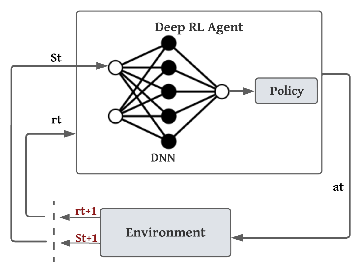
3. Learning VRFB Parameters Using Deep Reinforcement Learning

This section delves into the solution’s realization using the deep reinforcement learning algorithm and outlines the workflow and design phases.

3.1. Advancing to Deep Reinforcement Learning (Deep RL)

Reinforcement learning (RL) is a type of machine learning, unlike both supervised learning and unsupervised learning. RL is primarily centered around goal-directed learning, achieved through interactive experiences, making it distinct from traditional machine learning approaches [29,30]. Deep RL merges deep learning (DL) and RL, enabling artificial agents to acquire the capability to address problems involving sequential decision-making. In the past decade, deep RL has achieved remarkable results on a range of problems, especially optimization problems. It is considered a very fast-moving field, as it can effectively address a diverse array of intricate decision-making challenges and extend a machine’s capacity to tackle real-world problems with a level of intelligence akin to humans. Figure 5 illustrates the general structure of the RL agent’s interaction loop. At each step t, the agent is provided with a representation of the environment. State St selects an action based on a policy, and the environment responds to this action and presents a new situation or state to the agent. The environment, determined by the state/action pair, returns a reward, a specific numerical value that the agent aims to maximize over time by making optimal choices in its actions. The goal of the agent is to maximize the long-term rewards. In general, the agent consists of a policy and a learning algorithm that iteratively refines the policy to discover its optimal configuration. In the case of deep RL, the interaction loop is presented in Figure 6, where deep neural networks are used to find approximations for large, complex, and high-dimensional environments [30].

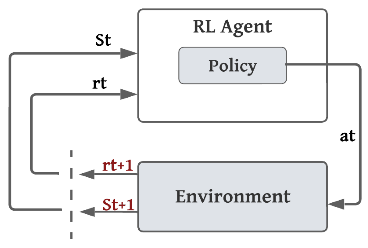
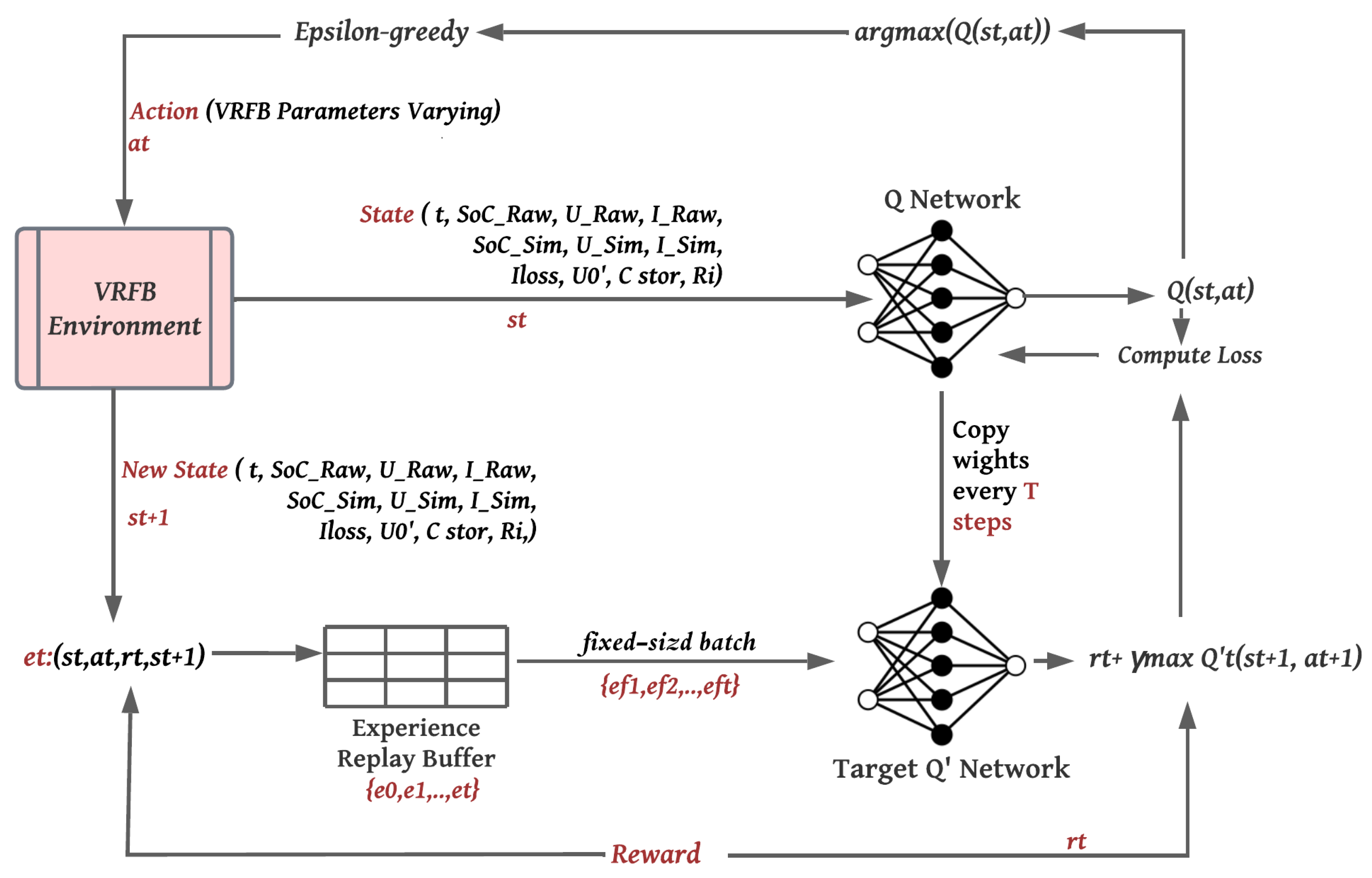
3.2. Markov Decision Process Formulation

We aim to determine the optimal VRFB-specific parameters that can ensure high accuracy of the reference simulation model [26]. Our solution involves varying and adjusting the VRFB-specific parameters—$I_{loss}$, $R_i$, $U_0^{\prime }$, and $C_{Stor}$—to find the best match or fit between the raw data with the simulated data produced by resolving the simulation model. We introduce a novel parameter-varying method using the deep q-learning algorithm. In the following discussion, we focus on the learning phase and define the general DQN agent that learns to determine the optimal battery-specific parameters. To this end, we train a deep RL agent to automatically adjust the VRFB-specific parameters to obtain the optimal values. In this context, the formulation of the RL problem is based on the Markov Decision Process (MDP), which serves as a straightforward framework for addressing the challenge of learning to accomplish a particular goal. Therefore, our goal is to determine the optimal VRFB-specific parameters that can ensure the high accuracy of the simulation model. Here, we define the important concepts of the MDP related to the DQN algorithm. Representing and modeling the system as an MDP is a crucial aspect in the design of a problem related to decision-making. Hence, throughout this work, we utilize the following elements:

∘

Environment: As our focus is on the VRFB, we consider the VRFB as the environment for our RL system. It includes essential details about the battery, such as its internal parameters and the extracted and preprocessed raw dataset.

∘

Agent: The agent uses the neural network to approximate the q-values through interactions with the VRFB environment.

∘

State: The state s is a tensor that includes the raw data, the simulated data produced by resolving the mathematical system, and the battery-specific parameters.

∘

Action Space: The action space reflects the adjustment and variation of the battery-specific parameters. Hence, our action space is a discrete space. In this context, we defined two different configurations of the action space. Initially, we outlined three possible actions, each involving adjusting the parameters: increasing $I_{loss}$, $R_i$, $U_0^{\prime }$, and $C_{Stor}$; decreasing them, or maintaining them. Subsequently, we expanded our action space to include nine distinct actions that refer to increasing, decreasing, or maintaining them separately. This method enabled us to determine which configuration produced better outcomes.

∘

Reward function: The agent learns the optimal battery-specific parameters that can enhance the simulation model’s accuracy. Thus, we were inspired by and utilized the reward function in [36]. We defined the following straightforward reward function given by the equation to encourage faster convergence and facilitate the learning process for the DQN agent.

$$r=\lambda (best\_ERROR-ERROR)$$

(4)

where:

∘

$\lambda$ is a hyperparameter;

∘

$best\_ERROR$ is the lowest error achieved so far during an episode;

∘

$ERROR$ includes the errors for the different battery state variables ($So{C}_{error}$, $U_{error}$, and $I_{error}$) multiplied by the weights ($w_{SoC}$, $w_U$, and $w_I$) for each variable, as described in Equation (5).

$$ERROR=w_{SoC}·|So{C}_{error}|+w_U·|U_{error}|+w_I·\left|I_{error}\right|$$

(5)

3.3. Training Algorithm for Deep Q-Network

Once we have formulated our MDP solution, we can present the whole DQN process for learning and determining the optimal VRFB-specific parameters. Figure 7 illustrates the general framework of the proposed method based on the DQN algorithm. At each step t, the agent receives some representation of the battery environment, state $s_t$, comprising the raw data ($So{C}_{Raw}$, $U_{Raw}$$I_{Raw}$), simulated data ($So{C}_{Sim}$, $U_{Sim}$$I_{sim}$), and battery parameters ($I_{loss}$, $R_i$, $U_0^{\prime }$, $C_{Stor}$). The agent is required to navigate the action space through the implementation of a policy, such as epsilon-greedy exploration. This exploration strategy allows the agent to choose between taking a random action with a probability of $ϵ$ or selecting an action based on the value function with the highest value, determined with a probability of $1-ϵ$. The agent selects an action (increase, decrease, or maintain the battery-specific parameters), and the environment responds to this action and presents a new state $s_{t+1}$ to the agent. Based on the state/action, a reward $r_t$ is provided that reflects its performance in fitting the simulated data with the raw data. In this process, the agent utilizes the predicted q-value, target q-value, and observed reward obtained from the data sample to calculate a loss. This loss is then employed to train the q-network.

To elaborate further, the training algorithm’s goal is to find the optimal action-value function $Q^{*}(s,a)$ that maximizes its expected return over the episode’s length.

The flowchart for training the DQN agent in our case is highlighted in Figure 8.

4. Results and Discussion

4.1. Training DQN Agent

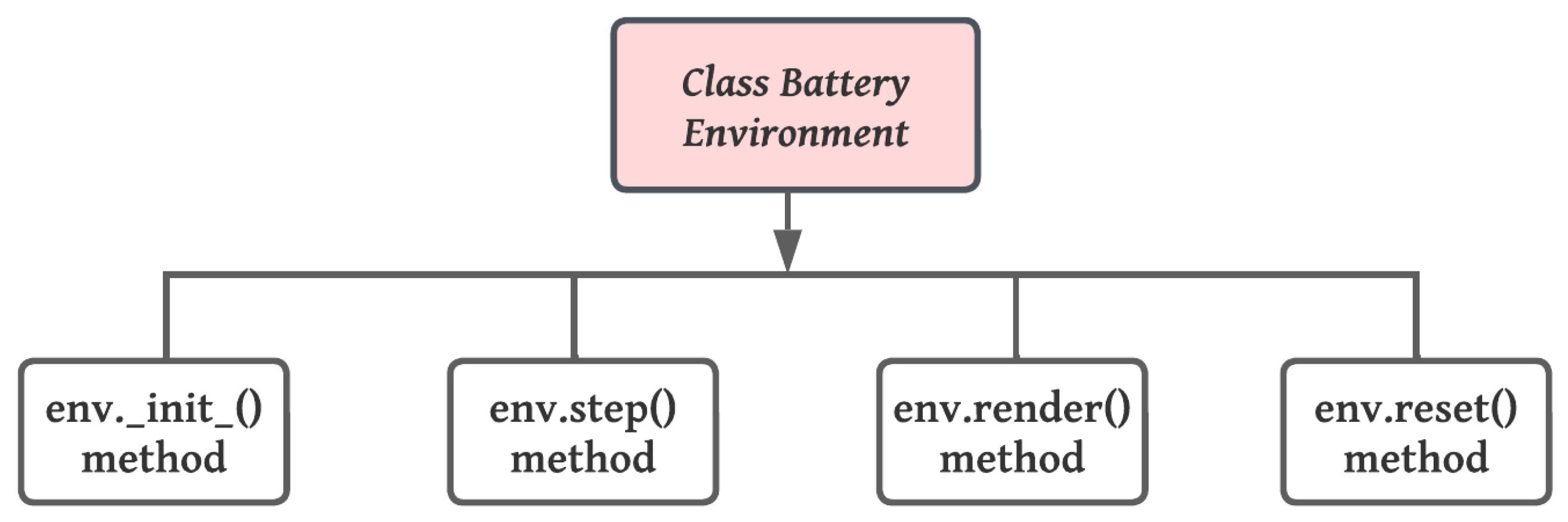
4.1.1. Definition of the Gym Environment

For the implementation of our custom environment, we used OpenAI Gym. OpenAI Gym provides an easy way to build environments for training RL agents [37]. The environment Gym class contains four methods, as illustrated in Figure 9:

∘

Initialization Method: The first method is the initialization method, where we create our environment class. We establish the action and state spaces and other initial battery parameter values within this function.

∘

Step Method: This method is run every single time we take a step within our environment involving taking and applying an action $a_t$ to the environment. This method returns the next state/observation $s_{t+1}$; the actual determined reward $r_t$; a Boolean variable done, which refers to the end of the episode; and the set info, which contains some additional information. In our case, we used the variable info to store the battery-specific parameters $I_{loss}$, $R_i$, $U_0^{\prime }$, and $C_{Stor}$.

∘

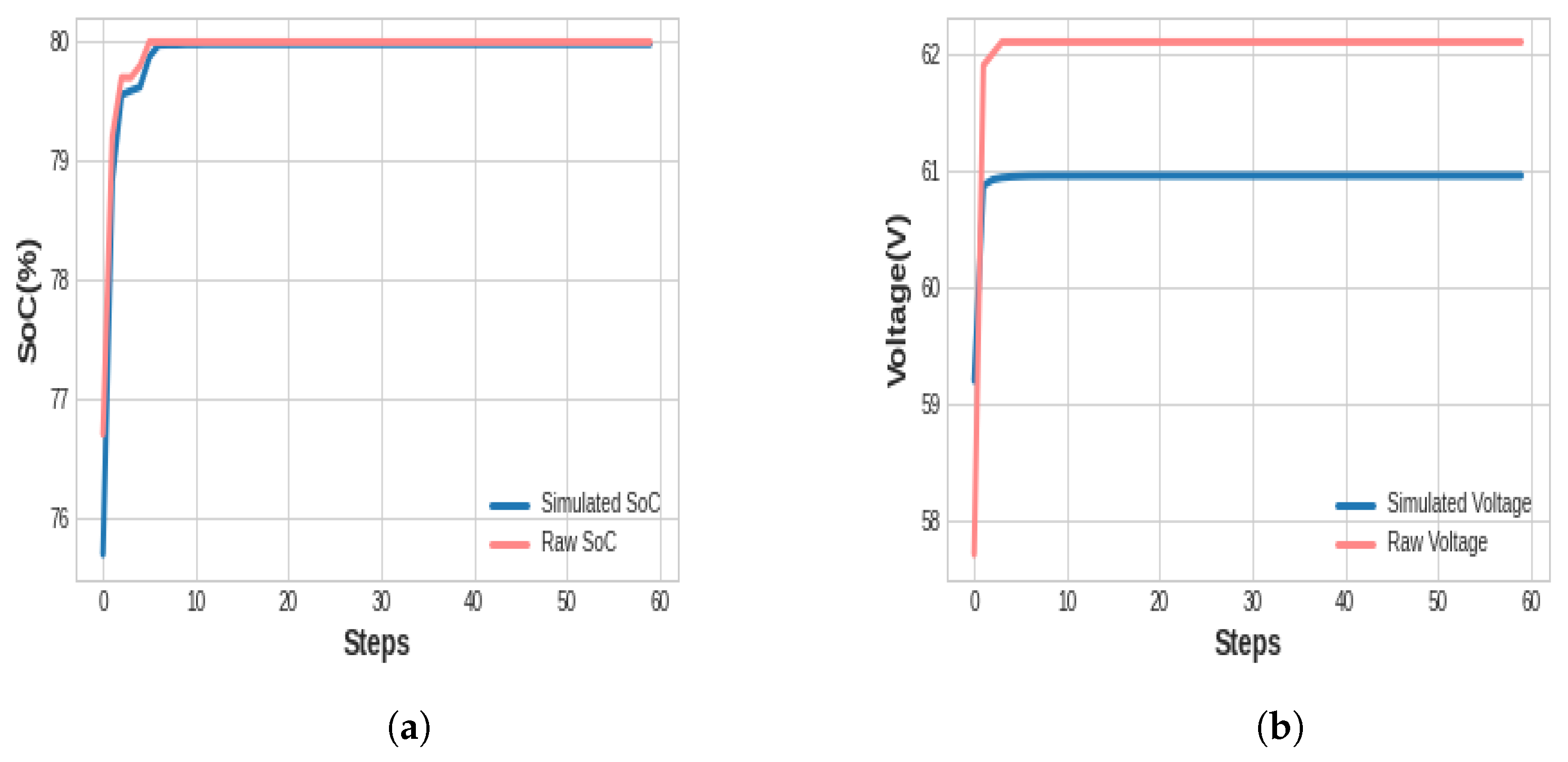
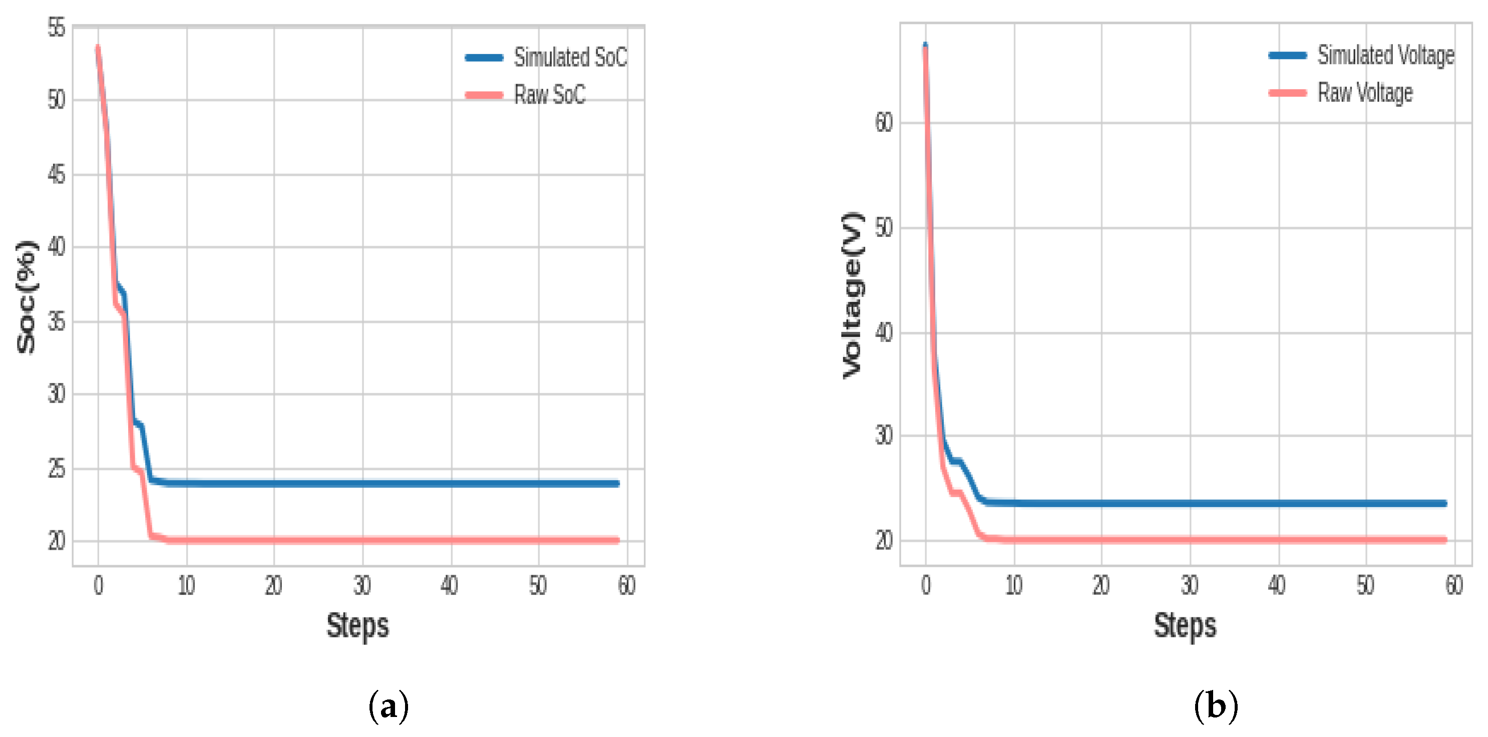
Render method: This method is used to visualize the current state. We used this method to track and display the alignment between the simulated data and the raw data during the episode.

∘

Reset method: Lastly, the reset method is where we reset the environment and obtain the initial observations.

4.1.2. DQN Parameters

Table 1. Initial values of VRFB parameters in the simulation model.

	Initial Value
SoC (%)	Charge: 20, Discharge: 80
${\mathit{C}}_{\mathit{Stor}}$  (As)	870,000
${\mathit{I}}_{\mathit{loss}}$  (A)	10.0
${\mathit{U}}_{\mathbf{0}}$  (V)	1.375
${\mathit{R}}_{\mathit{i}}$  (m$\mathsf{\Omega }$)	0.75
No. of stacks	10
Nominal Voltage (V)	48
Temperature (°C)	21.85
No. of Cells	40

illustrates the initial conditions and initial guesses used for solving the simulation model, as well as other relevant information used in the VRFB operating system. In fact, we kept the same values described and proposed in [26], as they are related to the same VRFB. For training the DQN agent, we considered the parameters for the neural networks and the RL system‘s parameters described in

Table 2. DQN agent and neural network parameters.

Parameter	Definition	Value
num_layers	Number of hidden layers used	2
num_units	Number of units used to enhance the quality of training and prediction	256.2
Activation Function	The non-linear activation function used for the NN	ReLU
Replace	The frequency with which the target network is updated	1000
Epsilon  $\mathit{ϵ}$	Level of probability randomness for each iteration	1.0
eps_min	The ending value of Epsilon	0.1
Decay_rate	Reducing the Epsilon at each iteration	1 × ${10}^{-5}$
Gamma   $\mathit{\gamma }$	Discount factor	0.99
Batch_size	Number of transitions sampled from the replay buffer	64
Learning_rate	The learning rate of the Adam optimizer	0.001

.

4.1.3. Training Results

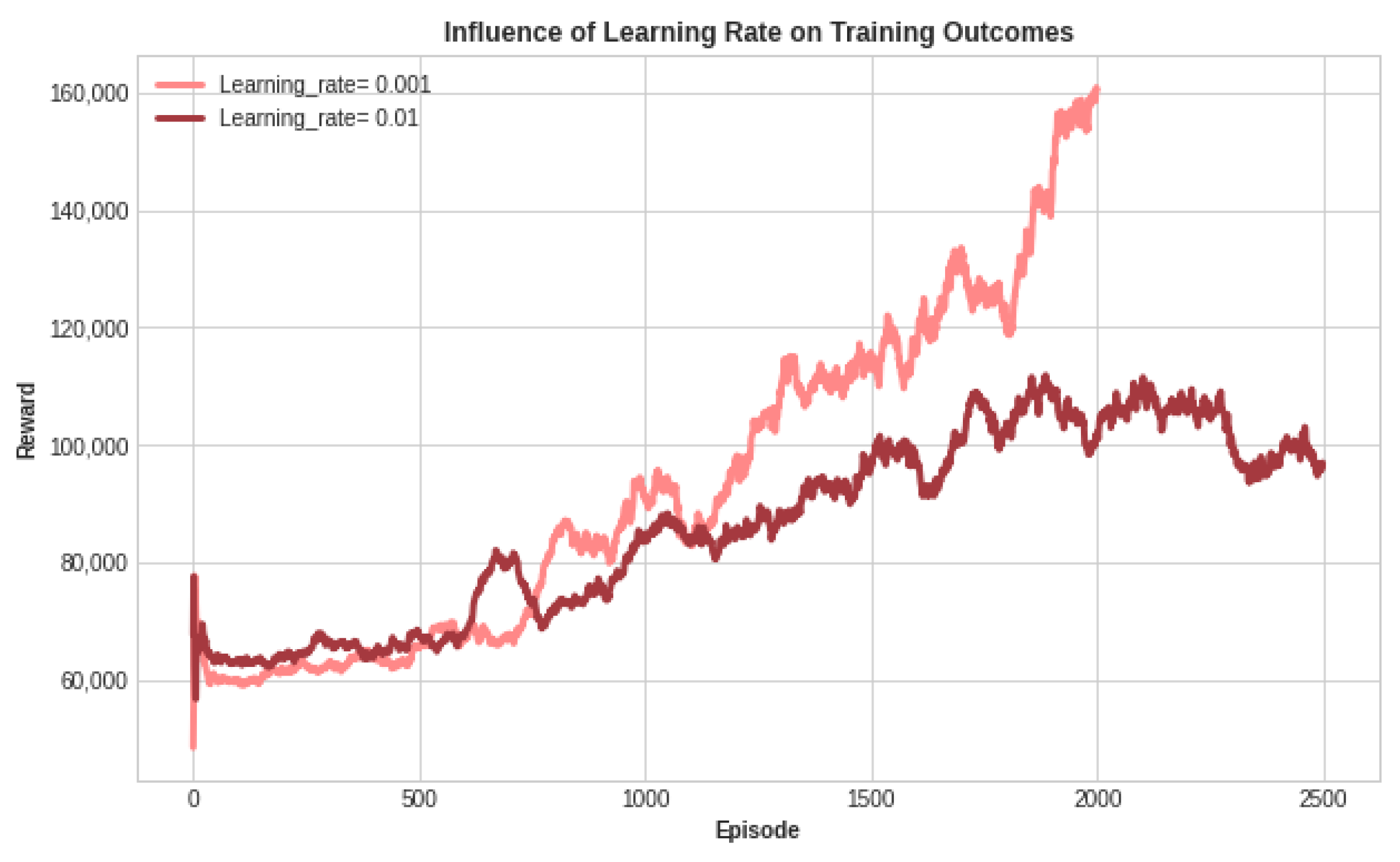
For the training phase, we trained the agent with the complete charging and discharging cases of a power cycle of P = 1 KW for 2500 episodes for both configurations of the action spaces. This means that only one power cycle at a time was selected to train the model.

a.

Optimizing the Learning Rate Selection for Training

Multiple iterations were performed to fine-tune the hyperparameters, including the learning rate shown in Figure 10. Based on our observations, it can be deduced that training the DQN agent with the learning rate set at 0.001 resulted in superior performance compared to the other configurations in terms of cumulative reward and rapid learning. Therefore, we chose to proceed with this value. The models were trained with the same neural network architecture, discount rate, and learning rate. During training, we created a model checkpoint each time we achieved a new highest cumulative reward within an episode.

b.

Choosing the Optimal Action Space

As previously discussed, we established and trained the DQN agent under two distinct action space configurations. The provided figures showcase the outcomes of the training process. Specifically, these figures display the accumulated average reward over 2500 episodes. Each episode consisted of 60 steps, indicating that the agent underwent 60 steps of action before resetting the environment and starting a new episode. Initially, we set all weights to 1. Subsequently, through training with various weight values for the battery state variables, we arrived at the following configuration to enhance the voltage prediction: ${\mathit{w}}_{\mathit{SoC}}$ = 0.3, ${\mathit{w}}_{\mathit{U}}$ = 0.5, and ${\mathit{w}}_{\mathit{I}}$ = 0.2. With fewer actions in the three-action space case, we aimed for a faster learning process. It is evident that the cumulative reward produced by fewer actions achieved better learning performance compared to the other configuration for both the charging and discharging processes, as demonstrated in Figure 11 and Figure 12. We can see that the average reward increased over training episodes, signifying effective learning by the DQN agent. In the three-action space case, the agent achieved a higher cumulative reward compared to the other case. The increased reward indicates that the agent is making progress in acquiring the desired task knowledge that reflects learning the optimal VRFB parameters.

Hence, our agent demonstrates improved performance when we simultaneously vary the parameters. Thus, the agent trained under the specific configuration of three valid actions was used for the subsequent evaluation phase.

4.2. Evaluation of the DQN Agent

Since the deep q-learning algorithm aims to find the optimal action-value function ${\mathit{Q}}^{*}(\mathit{s},\mathit{a})$,we need to verify and ensure that the trained model consistently produces higher accumulated rewards over a certain period. To ensure that deep q-learning produces a generalized model, we introduced the base DQN testing process.

4.2.1. DQN Agent Testing Process

The testing procedure in reinforcement learning differs from that in supervised or unsupervised machine learning. Debugging RL algorithms is very hard. To test whether it works well and the trained agent is good at its designated task, we need to apply the trained model to a defined situation or scenario. We present the testing process we considered to accomplish this in Figure 13. In addition, we defined the testing loop, as described by Algorithm 1.

Algorithm 1 General testing loop of our DQN agent

Reset the environment and get state ${\mathit{s}}_{\mathit{t}}$ for episode =1, M do do     Reset the environment and get the initial state ${\mathit{s}}_{\mathit{t}}$     while True do         Predict the action ${\mathit{a}}_{\mathit{t}}$ related to ${\mathit{s}}_{\mathit{t}}$         Execute a step s and get the next state ${\mathit{s}}_{\mathit{t}+\mathbf{1}}$, reward ${\mathit{r}}_{\mathit{t}}$, done, and info         Render the environment         if done then            Display optimal ${\mathit{I}}_{\mathit{loss}}$, ${\mathit{R}}_{\mathit{i}}$, ${\mathit{U}}_{\mathbf{0}}^{\prime }$, and ${\mathit{C}}_{\mathit{Stor}}$ stored in the variable info         end if     end while end for

As illustrated, the testing loop involves the prediction of the action, enabling the optimal configuration of the battery-specific parameters based on what has already been learned during the training phase. During each step, we rendered the environment to visualize how well the simulated data aligned with the raw data each time we executed the predicted action.

4.2.2. Testing Results and Evaluation

We assessed the performance of the trained DQN agent over a single episode containing 60 steps to evaluate its learning progress. The agent’s capabilities were tested using the other power cycles.

Table 3. Optimal parameters predicted by the DQN agent for the charging process.

Evaluation Power	Ri (m$\mathbf{\Omega }$)	U${}_{\mathbf{0}}^{\prime }$ (V)	I${}_{\mathit{Loss}}$ (A)	C${}_{\mathit{Stor}}$ (Ah)
2.5 kW	0.29	1.075	9.7	2415.83
5 kW	0.3	1.375	10.035	2416
7.5 kW	0.305	1.675	10.3	2417.5
10 kW	0.30	1.45	10.075	2416.88

presents the optimal values of the battery-specific parameters for each evaluation scenario. We highlighted the calculated RMSE values for the VRFB state variables between the simulated and raw data under the optimized parameter settings in

Table 4. Summary of test results assessing alignment between the raw and simulated data.

Evaluation Power	VRFB State Variables	RMSE	MAE
	State of charge SoC (%)	0.1114	0.029
2.5 kW	Voltage U (V)	1.923	1.8369
	Current I (A)	0.312	0.1028
	State of charge SoC (%)	0.2407	0.0723
5 kW	Voltage U (V)	1.8311	1.7832
	Current I (A)	0.2231	0.1031
	State of charge SoC (%)	0.8394	0.244
7.5 kW	Voltage U (V)	1.4741	1.468
	Current I (A)	0.3741	0.068
	State of charge SoC (%)	0.5573	0.1498
10 kW	Voltage U (V)	1.114	1.1204
	Current I (A)	0.113	0.0139

RMSE: root-mean-square error; MAE: mean absolute error.

.

As shown, we can conclude that the agent predicted the battery-specific parameters to perfectly match the data of the SoC with an RMSE value as low as 0.111% during testing on the 2.5 KW power cycle. Also, our agent predicted the optimal battery parameter values that best matched the voltage data, achieving the lowest RMSE value of 1.114 V during testing on the 10 KW power cycle.

Although the RMSE values for the voltage were higher compared to the SoC, we were able to improve the voltage prediction results in [26]. To illustrate these improvements,

Table 5. Summary of test results of our approach and the reference method for the charging process.

Approach	Evaluation Power	WLSS (%)
Model [26]	2.5 KW	187.58
	5 KW	100.14
	7.5 KW	7.9
	10 KW	120.51
DQN Agent	2.5 KW	170.42
	5 KW	87.51
	7.5 KW	6.07
	10 KW	90.41

provides a comparative analysis between our approach and the reference model, using the weighted least-squares similarity (WLSS) as the evaluation metric to align with the metric used in [26]. The WLSS is defined by Equation (6).

$$\mathit{WLSS}\left(\mathit{p}\right)=(\frac{\mathit{LSS}\left(\mathit{p}\right)}{\mathit{minLSS}\left(\mathit{p}\right)}-\mathbf{1})\times \mathbf{100}\%$$

(6)

where $\mathit{p}$ is the selected power cycle, $\mathit{LSS}$ is taken from Equation (7), and $\mathit{minLSS}$ is the lowest LSS achieved so far.

$$\mathit{LSS}={\mathit{SoC}}_{\mathit{error}}+{\mathit{U}}_{\mathit{error}}+{\mathit{I}}_{\mathit{error}}$$

(7)

As evident from Table 5, it is crystal clear that we achieved superior performance compared to the method outlined in [26], as the DQN agent facilitated a reduction in the WLSS (%) for nearly all evaluation scenarios. As a result, our DQN agent achieved an improvement of nearly 10% compared to the reference work. To provide a more comprehensive illustration, Figure 14 demonstrates the results of fitting the simulated data with the raw data while testing the DQN agent specifically on the 10 kW power cycle for the state variables (SoC and voltage) for the charging process. Figure 15 demonstrates the same results but for the discharging process. It is important to note that these figures present the predicted state variable for each step of the episode.

4.2.3. Discussion

Based on Table 3 and the accompanying figures, it is evident that the DQN agent is capable of predicting battery-specific parameters with the lowest RMSE and MAE values, outperforming the results achieved in [26]. Nonetheless, there is room for improvement, especially in the voltage prediction. In our pursuit of improving the results, we decided to delve deeper into optimizing the DQN agent.

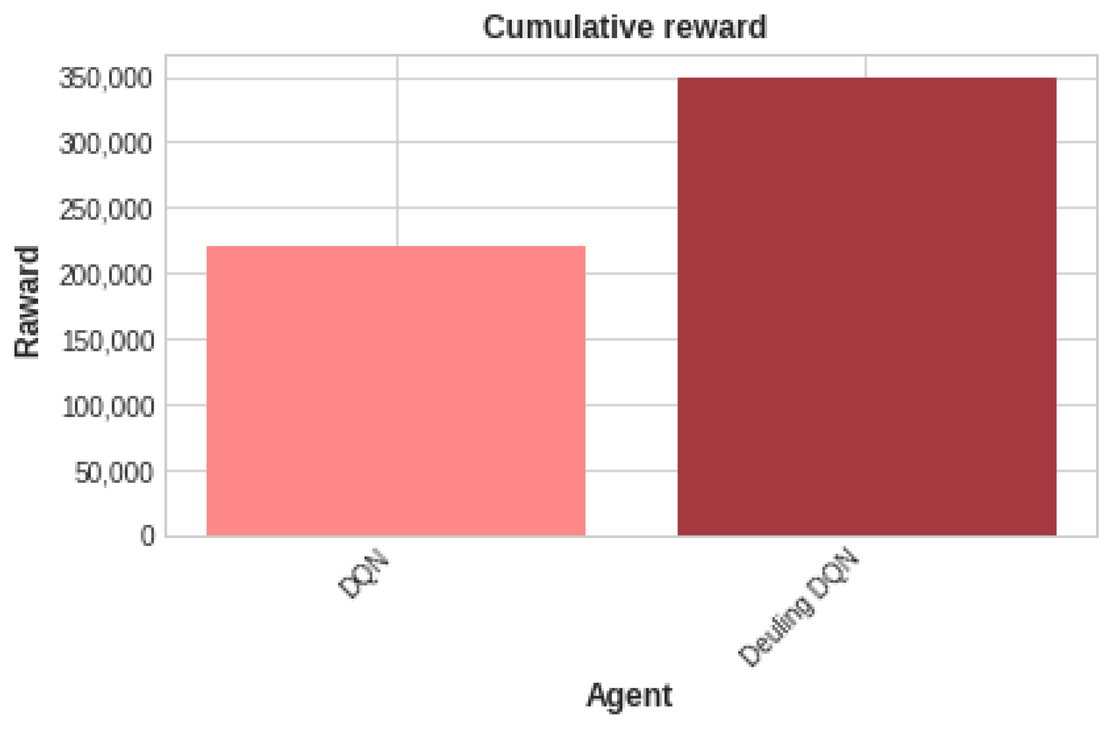
4.3. Enhancing the Performance of the DQN Agent

Several improvements of the deep q-network have been proposed in the literature [38,39]. Specifically, the Rainbow DQN incorporates a thorough analysis of six impactful q-learning techniques [39]. These enhancements encompass double DQN, dueling DQN, prioritized experience replay, multi-step learning, distributional DQN, and NoisyNet. Among them, we chose to enhance our DQN by implementing the dueling DQN, as its novelty lies in the q-network architecture, and its implementation is similar to the DQN [40]. Its linear layers split into value and advantage streams. The combination of these two streams is achieved through a dedicated aggregating layer, resulting in the estimation of the state-action value function Q. Figure 16 illustrates the cumulative reward achieved after training the dueling DQN agent using parameters and configurations identical to those of the DQN agent. It is evident that the dueling DQN agent outperformed the DQN agent and excelled in learning compared to the DQN agent, as it accumulated a higher reward.

Therefore, we conducted a comparative analysis between the DQN agent and the dueling DQN agent for predicting the VRFB voltage using a power cycle of 10 kW for the charging process, as presented in

Table 6. Comparative analysis of voltage predictions.

Metric	DQN	Dueling DQN
RMSE [V]	1.114	1.1081
MAE [V]	1.1204	1.0914

, whereas

Table 7. Comparative analysis of state-of-charge predictions.

Metric	DQN	Deuling DQN
RMSE [%]	0.5573	0.456
MAE [%]	0.1498	0.0932

presents a similar comparison for the SoC predictions using the same power cycle. Despite the marginal reduction in the RMSE and MAE when employing the dueling DQN, it consistently outperformed the DQN agent by accumulating higher rewards, thereby improving the performance of the DQN agent by nearly 10%.

5. Conclusions

This work is our contribution to the optimization and performance improvement of the VRFB simulation model. In this process, we expanded the optimization of the simulation model by varying its specific parameters. We advocated a deep q-network agent to determine the optimal VRFB-specific parameters, reduce the required scope of the input data, and enhance the accuracy of the simulation model. We allowed the DQN agent to learn autonomously to determine the battery-specific parameters that can ensure the best fit between the raw data and the simulated data produced by resolving the battery’s mathematical system, thereby enhancing the simulation model’s accuracy. These parameters are considered the optimal battery-specific parameters, as they were predicted while testing the DQN agent in specific power cycles after its training and learning processes.

In this paper, we began by presenting the context of our work, and then we walked through the existing solution for modeling and optimizing the simulation of VRFB batteries. We introduced our proposed method in response to this problem. We showcased that our proposed method exhibited good performance, achieving lower RMSE values of 0.111% for the SoC and 1.114 V for the voltage. In addition, it outperformed the optimization results of the method used in the prediction of battery state variables and the determination of optimal battery parameters, especially voltage, in [26].

We illustrated this by testing multiple power cycles measured for a specific VRFB. The testing results demonstrated that our trained DQN agent is robust and does not suffer from overfitting to the training conditions. We then worked on improving our results by applying the dueling DQN, resulting in a notable improvement of 10%. This optimized simulation model can be generalized to other types of redox-flow batteries. In addition to the outstanding performance of our learned VRFB parameters, our concept proved to be simple and easy to adapt when the optimization goals need to be changed. In other words, it is possible to change the target of change in the optimization process and we may just adapt the reward function and let our RL agent train autonomously again.

There are several extension possibilities for this work, ranging from optimizing the current results to extending the work with new concepts. To optimize the current results, we suggest several ideas. The first would be to alternate the deep RL algorithms suggested in Rainbow that combine several improvements of deep RL algorithms [39]. We only tried the dueling deep q-network due to time limitations. The second would be to configure and fine-tune the hyperparameters, as during this work, the hyperparameters of the deep RL agent were not well exploited. We expect better performance with better hyperparameter configuration and tuning.

References

1. Global Energy. Available online: https://www.iea.org/energy-system/transport/electric-vehicles (accessed on 15 July 2023).
2. Sutikno, T.; Arsadiando, W.; Wangsupphaphol, A.; Yudhana, A.; Facta, M. A review of recent advances on hybrid energy storage system for solar photovoltaics power generation. IEEE Access 2022, 10, 42346–42364. [Google Scholar] [CrossRef]
3. Ferret, R.; Sánchez-Díez, E.; Ventosa, E.; Guarnieri, M.; Trovò, A.; Flox, C.; Marcilla, R.; Soavi, F.; Mazur, P.; Aranzabe, E. Redox flow batteries: Status and perspective towards sustainable stationary energy storage. J. Power Sources 2021, 481, 228804. [Google Scholar]
4. Skyllas-Kazacos, M. All-Vanadium Redox Battrey; MIT Press: Cambridge, MA, USA, 1986. [Google Scholar]
5. Rizzuti, A.; Carbone, A.; Dassisti, M.; Mastrorilli, P.; Cozzolino, G.; Chimienti, M.; Olabi, A.G.; Matera, F. Vanadium: A Transition Metal for Sustainable Energy Storing in Redox Flow Batteries; ELSEVIER: Amsterdam, The Netherlands, 2016. [Google Scholar]
6. Di Noto, V.; Sun, C.; Negro, E.; Vezzù, K.; Pagot, G.; Cavinato, G.; Nale, A.; Bang, Y.H. Hybrid Inorganic-Organic Proton-Conducting Membranes Based on SPEEK Doped with WO3 Nanoparticles for Application in Vanadium Redox Flow Batteries; Electrochimica Acta, ELSEVIER: Amsterdam, The Netherlands, 2019. [Google Scholar]
7. Neves, L.P.; Gonçalves, J.; Martins, A. Methodology for Real Impact Assessment of the Best Location of Distributed Electric Energy Storage; Sustainable Cities and Society; Elsevier: Amsterdam, The Netherlands, 2016. [Google Scholar]
8. Schubert, C.; Hassen, W.F.; Poisl, B.; Seitz, S.; Schubert, J.; Usabiaga, E.O.; Gaudo, P.M.; Pettinger, K.H. Hybrid Energy Storage Systems Based on Redox-Flow Batteries: Recent Developments, Challenges, and Future Perspectives. Batteries 2023, 9, 211. [Google Scholar] [CrossRef]
9. Skyllas-Kazacos, M.; Xiong, B.; Zhao, J.; Wei, Z. Extended Kalman filter method for state of charge estimation of vanadium redox flow battery using thermal-dependent electrical model. J. Power Sources 2014, 262, 50–61. [Google Scholar]
10. He, F.; Shen, W.X.; Kapoor, A.; Honnery, D.; Dayawansa, D. H infinity observer based state of charge estimation for battery packs in electric vehicles. In Proceedings of the 2016 IEEE 11th Conference on Industrial Electronics and Applications (ICIEA), Hefei, China, 5–7 June 2016. [Google Scholar]
11. Hannan, M.A.; Lipu, M.H.; Hussain, A.; Mohamed, A. A review of lithium-ion battery state of charge estimation and management system in electric vehicle applications: Challenges and recommendations. Renew. Sustain. Energy Rev. 2017, 78, 834–854. [Google Scholar] [CrossRef]
12. Costa-Castell’o, R.; Strahl, S.; Luna, J. Chattering free sliding mode observer estimation of liquid water fraction in proton exchange membrane fuel cells. J. Frankl. Inst. 2017, 357, 13816–13833. [Google Scholar]
13. Clemente, A.; Cecilia, A.; Costa-Castelló, R. SOC and diffusion rate estimation in redox flow batteries: An I&I-based high-gain observer approach. In Proceedings of the 2021 European Control Conference (ECC), Rotterdam, The Netherlands, 29 June–2 July 2021. [Google Scholar]
14. Battaiotto, P.; Fornaro, P.; Puleston, T.; Puleston, P.; Serra-Prat, M.; Costa-Castelló, R. Redox flow battery time-varying parameter estimation based on high-order sliding mode differentiators. Int. J. Energy Res. 2022, 46, 16576–16592. [Google Scholar]
15. Clemente, A.; Montiel, M.; Barreras, F.; Lozano, A.; Costa-Castello, R. Vanadium redox flow battery state of charge estimation using a concentration model and a sliding mode observer. IEEE Access 2021, 9, 72368–72376. [Google Scholar] [CrossRef]
16. Choi, Y.Y.; Kim, S.; Kim, S.; Choi, J.I. Multiple parameter identification using genetic algorithm in vanadium redox flow batteries. J. Power Sources 2020, 45, 227684. [Google Scholar] [CrossRef]
17. Wan, S.; Liang, X.; Jiang, H.; Sun, J.; Djilali, N.; Zhao, T. A coupled machine learning and genetic algorithm approach to the design of porous electrodes for redox flow batteries. Appl. Energy 2021, 298, 117177. [Google Scholar] [CrossRef]
18. Niu, H.; Huang, J.; Wang, C.; Zhao, X.; Zhang, Z.; Wang, W. State of charge prediction study of vanadium redox-flow battery with BP neural network. In Proceedings of the 2020 IEEE International Conference on Artificial Intelligence and Computer Applications (ICAICA), Dalian, China, 27–29 June 2020; pp. 1289–1293. [Google Scholar]
19. Cao, H.; Zhu, X.; Shen, H.; Shao, M. A neural network based method for real-time measurement of capacity and SOC of vanadium redox flow battery. In Proceedings of the International Conference on Fuel Cell Science, Engineering and Technology, American Society of Mechanical Engineers, San Diego, CA, USA, 28 June–2 July 2015; Volume 56611, p. V001T02A001. [Google Scholar]
20. Heinrich, F.; Klapper, P.; Pruckner, M. A comprehensive study on battery electric modeling approaches based on machine learning. J. Power Sources 2021, 4, 17. [Google Scholar] [CrossRef]
21. Iu, H.; Fernando, T.; Li, R.; Xiong, B.; Zhang, S.; Zhang, X.; Li, Y. A novel one dimensional convolutional neural network based data-driven vanadium redox flow battery modelling algorithm. J. Energy Storage 2023, 61, 106767. [Google Scholar]
22. Iu, H.; Fernando, T.; Li, R.; Xiong, B.; Zhang, S.; Zhang, X.; Li, Y. A Novel U-Net based Data-driven Vanadium Redox Flow Battery Modelling Approach. Electrochim. Acta 2023, 444, 141998. [Google Scholar]
23. Hannan, M.A.; How, D.N.; Lipu, M.H.; Mansor, M.; Ker, P.J.; Dong, Z.; Sahari, K.; Tiong, S.K.; Muttaqi, K.M.; Mahlia, T.I.; et al. Deep learning approach towards accurate state of charge estimation for lithium-ion batteries using self-supervised transformer model. Sci. Rep. 2021, 11, 19541. [Google Scholar] [CrossRef] [PubMed]
24. Zhang, C.; Li, T.; Li, X. Machine learning for flow batteries: Opportunities and challenges. Chem. Sci. 2022, 17, 4740–4752. [Google Scholar]
25. Wei, Z.; Xiong, R.; Lim, T.M.; Meng, S.; Skyllas-Kazacos, M. Online monitoring of state of charge and capacity loss for vanadium redox flow battery based on autoregressive exogenous modeling. J. Power Sources 2018, 402, 252–262. [Google Scholar] [CrossRef]
26. Zugschwert, C.; Dundálek, J.; Leyer, S.; Hadji-Minaglou, J.R.; Kosek, J.; Pettinger, K.H. The Effect of input parameter variation on the accuracy of a Vanadium Redox Flow Battery Simulation Model. Batteries 2021, 7, 7. [Google Scholar] [CrossRef]
27. Weber, R.; Schubert, C.; Poisl, B.; Pettinger, K.H. Analyzing Experimental Design and Input Data Variation of a Vanadium Redox Flow Battery Model. Batteries 2023, 9, 122. [Google Scholar] [CrossRef]
28. He, Q.; Fu, Y.; Stinis, P.; Tartakovsky, A. Enhanced physics-constrained deep neural networks for modeling vanadium redox flow battery. J. Power Sources 2022, 542, 231807. [Google Scholar] [CrossRef]
29. Sutton, R.S.; Barto, A.G. Reinforcement Learning: An Introduction, 2nd ed.; The MIT Press: Cambridge, MA, USA, 2020. [Google Scholar]
30. Plaat, A. Deep Reinforcement Learning; Springer Nature Singapore Pte Ltd.: Singapore, 2022. [Google Scholar]
31. König, S. Model-Based Design and Optimization of Vanadium Redox Flow Batteries; Karlsruher Instituts für Technologie: Karlsruhe, Germany, 2017. [Google Scholar]
32. Haisch, T.; Ji, H.; Weidlichm, C. Monitoring the state of charge of all-vanadium redox flow batteries to identify crossover of electrolyte. Electrochim. Acta 2020, 336, 135573. [Google Scholar] [CrossRef]
33. Loktionov, P.; Konev, D.; Pichugov, R.; Petrov, M.; Antipov, A. Calibration-free coulometric sensors for operando electrolytes imbalance monitoring of vanadium redox flow battery. J. Power Sources 2023, 553, 232242. [Google Scholar] [CrossRef]
34. Shin, K.H.; Jin, C.S.; So, J.Y.; Park, S.K.; Kim, D.H.; Yeon, S.H. Real-time monitoring of the state of charge (SOC) in vanadium redox-flow batteries using UV–Vis spectroscopy in operando mode. J. Energy Storage 2020, 27, 101066. [Google Scholar] [CrossRef]
35. Cellstrom GmbH. Available online: https://unternehmen.fandom.com/de/wiki/Cellstrom_GmbH (accessed on 15 June 2023).
36. Subramanian, S.; Ganapathiraman, V.; El Gamal, A. Learned Learning Rate Schedules for Deep Neural Network Training Using Reinforcement Learning; Amazon Science, ICLR: Los Angeles, CA, USA, 2023. [Google Scholar]
37. Gym Library. Available online: https://www.gymlibrary.dev/content/basic_usage/ (accessed on 5 May 2023).
38. DQN Improvement. Available online: https://dl.acm.org/doi/fullHtml/10.1145/3508546.3508598#:~:text=In%20a%20discrete%20or%20continuous,k%7D%2C%20k%20%E2%88%88%20R (accessed on 22 April 2023).
39. Hessel, M.; Modayil, J.; Van Hasselt, H.; Schaul, T.; Ostrovski, G.; Dabney, W.; Horgan, D.; Piot, B.; Azar, M.; Silver, D. Rainbow: Combining improvements in deep reinforcement learning. In Proceedings of the AAAI Conference on Artificial Intelligence, New Orleans, LA, USA, 2–7 February 2018; Volume 32. [Google Scholar]
40. Wang, Z.; Schaul, T.; Hessel, M.; Hasselt, H.; Lanctot, M.; Freitas, N. Dueling network architectures for deep reinforcement learning. In Proceedings of the International Conference on Machine Learning, New York, NY, USA, 20–22 June 2016; pp. 1995–2003. [Google Scholar]
Figure 1. Comprehensive categorization of estimation algorithms for VRFB systems.
Batteries 10 00008 g001
Figure 2. Steps of the simulation model proposed in [26].
Batteries 10 00008 g002
Figure 3. Distribution of raw charging data.
Batteries 10 00008 g003
Figure 4. Distribution of raw discharging data.
Batteries 10 00008 g004
Figure 5. General structure of RL agent’s interaction loop.
Batteries 10 00008 g005
Figure 6. General structure of deep RL agent’s interaction loop.
Batteries 10 00008 g006
Figure 7. General framework of the proposed method based on the DQN algorithm.
Batteries 10 00008 g007
Figure 8. Flowchart for training the DQN agent.
Batteries 10 00008 g008
Figure 9. Methods of the battery environment class.
Batteries 10 00008 g009
Figure 10. Exploring the learning rate’s influence on the training outcomes.
Batteries 10 00008 g010
Figure 11. Cumulative reward for the charging process for both configurations of the action space.
Batteries 10 00008 g011
Figure 12. Cumulative reward for the discharging process for both configurations of the action space.
Batteries 10 00008 g012
Figure 13. Testing process of the DQN agent.
Batteries 10 00008 g013
Figure 14. Comparison of simulated and raw data using P = 10 KW for the charging process. (a) SoC testing outcome for the charging process. (b) Voltage testing outcome for the charging process.
Batteries 10 00008 g014
Figure 15. Comparison of simulated and raw data using P = 10 KW for the discharging process. (a) SoC testing outcome for the discharging process. (b) Voltage testing outcome for the discharging process.
Batteries 10 00008 g015
Figure 16. Cumulative rewards for DQN and dueling DQN.
Batteries 10 00008 g016