Real-Time Lithium Battery Aging Prediction Based on Capacity Estimation and Deep Learning Methods

Abstract

Lithium-ion batteries are key elements in the development of electrical energy storage solutions. However, due to cycling, environmental, and operating conditions, battery capacity tends to degrade over time. Capacity fade is a common indicator of battery state of health (SOH) because it is an indication of how the capacity has been degraded. However, battery capacity cannot be measured directly, and thus, there is an urgent need to develop methods for estimating battery capacity in real time. By analyzing the historical data of a battery in detail, it is possible to predict the future state of a battery and forecast its remaining useful life. This study developed a real-time, simple, and fast method to estimate the cycle capacity of a battery during the charge cycle using only data from a short period of each charge cycle. This proposal is attractive because it does not require data from the entire charge period since batteries are rarely charged from zero to full. The proposed method allows for simultaneous and accurate real-time prediction of the health and remaining useful life of the battery over its lifetime. The accuracy of the proposed method was tested using experimental data from several lithium-ion batteries with different cathode chemistries under various test conditions.

1. Introduction

Lithium-ion (Li-ion) batteries are the cornerstone in the development of electrical energy storage solutions [1]. Today, Li-ion batteries offer high specific energy, high efficiency (>95%), long cycle life, up to thousands of charge/discharge cycles [2], and low self-discharge rate [3,4]. Several cathode chemistries coexist, including lithium manganese oxide (LMO) batteries (up to 1500 cycles and 140 Wh/kg), lithium iron phosphate (LFP) batteries (up to 2000 cycles and 140 Wh/kg), nickel manganese cobalt oxide (NMC) batteries (up to 2000 cycles and 240 Wh/kg), and lithium nickel cobalt aluminum oxide (NCA) batteries (up to 1500 cycles and 250 Wh/kg). Recently, NMC cells have reported energy densities exceeding 300 Wh/kg [5].

As a result, Li-ion batteries are widely used in a variety of applications, including transportation systems, electronics, and grid storage, among others [6]. Battery degradation is a complex phenomenon that depends on thermal, mechanical, and electrochemical processes, whose behaviors depend on battery chemistry, cell design, operating conditions, and use patterns [7,8]. As a result, extending the battery life is a complex and challenging research topic that has a significant potential impact on the reliability and performance of battery-powered systems. Battery life extension strategies are receiving increased attention [9], as extended battery life can reduce operating costs and environmental impact while enabling more sustainable operation of battery systems [10,11].

To ensure their optimal use, extend their life, improve the maintenance schedules of the battery-powered equipment [12], and minimize the environmental impact associated with battery disposal, accurate state of health (SOH) estimation and prediction is critical. The SOH is a key indicator for awareness of the battery condition and battery derating control [8]. In [13], the SOH is defined as the Q^max/Q^rated ratio, where Q^max is the maximum charge the battery can hold at the present time and Q^rated is the nominal or rated charge.

New cells can typically withstand higher load currents, but as they age, the same current can cause accelerated degradation. At the beginning of its life, a battery can be charged at a certain current rate without problems, but as it ages, an increase in internal resistance, loss of active material, or other phenomena can lead to undesirable effects, such as lithium plating at the same charge current [14]. As a result, it is necessary to determine the SOH and remaining useful life (RUL) of the battery as it ages. This allows for preventive and operational actions to be planned. Batteries are often considered to be at the end of their life when they have approximately 70% to 80% of their initial or reference capacity [15].

The rated capacity of a battery, which is usually specified by the manufacturer, is defined as the amount of charge that a fully charged battery can deliver under specified load and temperature conditions [16]. However, due to cycling, operating, and environmental conditions, the capacity of a battery will differ from the rated capacity due to battery fade resulting from battery use. For example, high discharge rates tend to increase the energy loss and internal resistance of a battery, resulting in reduced cycle capacity. Therefore, the cycle capacity is an indicator of the amount of charge the battery can hold, similar to the fuel gauge in internal combustion vehicles [3], and thus, it is an accepted indicator of the SOH of a battery. Since it cannot be directly measured, real-time methods to estimate the cycle capacity of a battery are a must. With the widespread application of renewable energy sources and electric vehicles, researchers have paid much attention to the development of accurate battery RUL models [17].

Several methods were proposed to estimate battery capacity and can be roughly classified as direct and indirect methods, while the latter ones can be subclassified as analysis-based methods, state of charge (SOC)-based methods, and data-driven methods [17].

The simplest method, known as Coulomb counting, is based on the accumulation of the charge over its cycling period [18]. This direct method requires a full charge or discharge of the battery under specific conditions described in various IEC [19], ISO [20], and IEEE [21] standards since a direct measurement cannot predict the battery capacity in real applications when the battery is partially charged or discharged [17]. Another direct method is based on measuring the internal resistance of the battery, which can be measured by applying a current pulse to the battery, as this allows the capacity of the battery to be estimated [22].

Indirect methods require sensors to measure the current, voltage, and temperature and use these variables to estimate the capacitance. Analysis-based methods include electrochemical impedance spectroscopy, differential voltage, incremental curve, differential thermal curve, and mechanical stress, among others. SOC-based methods can be divided into indirect-estimation- and observer-based methods. While indirect SOC-based methods often estimate the battery capacity using the change in SOC determined by applying the Coulomb counting method over a period, observer-based SOC methods estimate the battery capacity directly using an observer based on an equivalent circuit of the battery. Finally, data-driven methods use mathematical tools, such as neural networks, support vector machines, Bayesian learning, or deep learning, to analyze large amounts of data to estimate the battery capacity without the need to pre-specify a particular battery model [17].

This paper proposes a real-time, simple, and fast method to determine the cycle capacity or maximum charge that the battery can currently hold for any SOH during the battery charge cycle using voltage and current measurements during a short interval of the charge cycle. This approach is attractive because the charge cycle is controlled by the battery management system (BMS) according to a known strategy (constant current followed by a constant voltage stage), and the proposed approach does not require data from the entire charge period, as batteries are rarely charged from zero to full charge. The proposed approach requires only a small amount of data from each charge cycle, balancing the accuracy, efficiency, and low computational burden, while allowing the current battery SOH to be known without the need for extensive and resource-intensive measurements.

Furthermore, the proposed approach is used to predict the degradation of the battery in conjunction with other state-of-the-art predictive techniques, such as recurrent neural networks (RNNs) [23,24]. RNNs are a deep learning approach for modeling sequential data, which are particularly well-suited for capturing the temporal dependencies of data sets and making them effective for modeling the dynamic evolution of a battery’s SOH over time.

The proposed strategy allows for simultaneous and real-time accurate prediction of SOH and capacity degradation over a battery’s lifetime. This approach not only provides a real-time assessment of the battery’s health but also offers a forward-looking perspective that aids in the predictive maintenance and management of battery systems, which can be particularly useful in applications where reliability and longevity are critical factors.

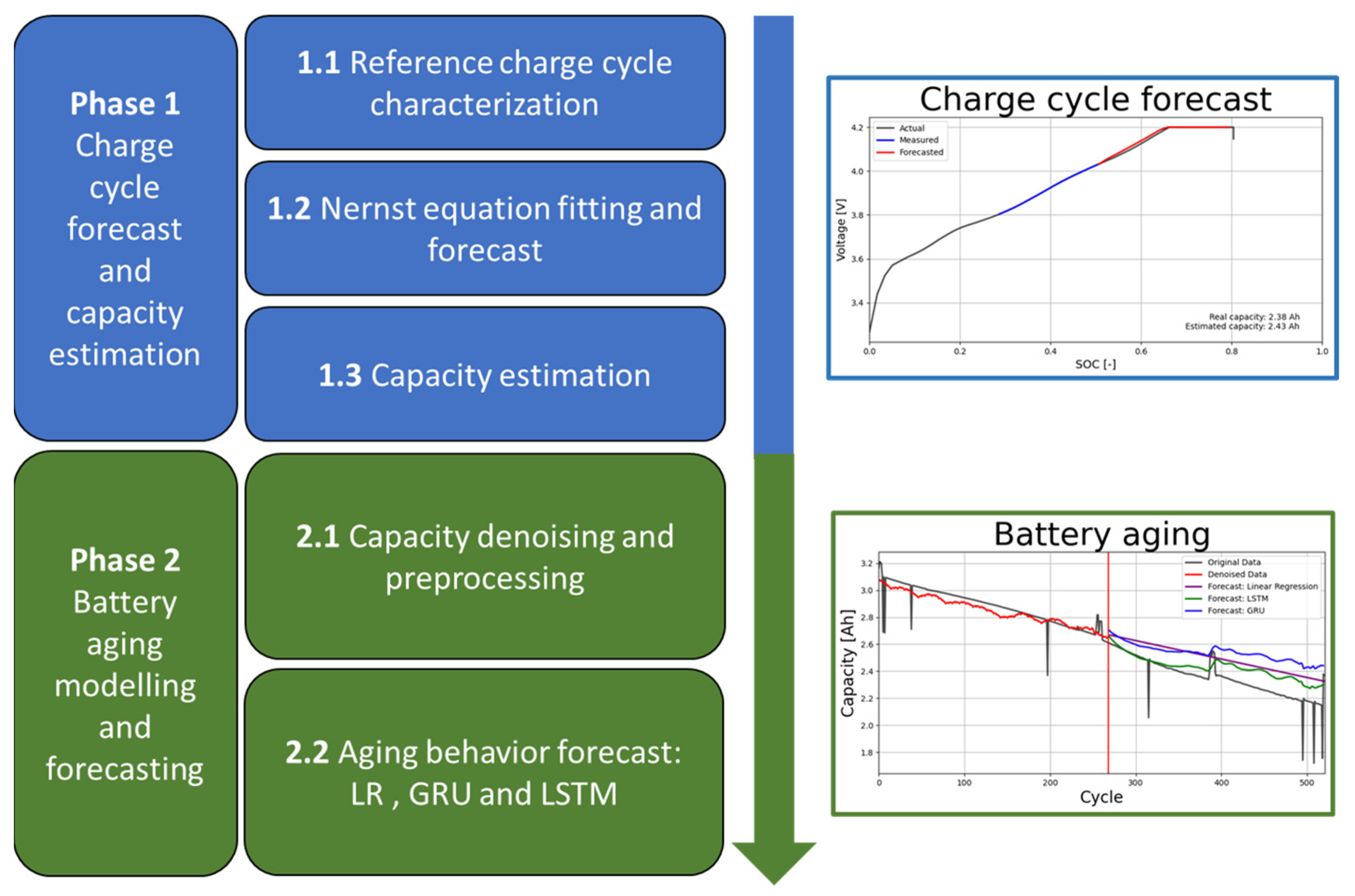
The remainder of the paper is organized as follows. Section 2 describes the methodology proposed in this paper to determine the SOH and degradation of the analyzed batteries. Section 3 describes the battery data set used in this paper. Section 4 presents and discusses the experimental results, and finally, Section 5 concludes this paper.

2. Methodology

Capacity, in the context of batteries, refers to the maximum amount of electric charge a battery can store. Capacity is a critical parameter that evolves over time and directly affects a battery’s energy storage capability and service life, making it an indicator to quantify battery degradation.

The capacity is typically measured in ampere-hours [Ah] and represents the total charge a battery can deliver under specific load and temperature conditions. It can be defined as [15]

$$C={\displaystyle {\int }_{t_0}^{t_f}i(t)dt} [\mathrm{Ah}]$$

(1)

The capacity fade after n charge/discharge cycles △C_n is a key indicator of battery degradation. It is defined as the reduction in available battery capacity (cycle capacity) over time and is expressed as the difference between the initial or reference capacity of a fresh battery, i.e., C^ref (reference capacity), and the remaining capacity at cycle n, i.e., $C^n$, as

$$\mathsf{\Delta }{C}^n=C^{{}_{ref}}-C^n [\mathrm{Ah}]$$

(2)

Monitoring the capacity changes provides valuable insight into the mechanisms affecting the electrodes and electrolyte and the degradation of the cell. The evolution of the capacity can then be used as the input for forecasting techniques, such as LR and an RNN.

In this paper, the state of charge of a battery at a given time, i.e., SOC(t), is defined as the ratio between the remaining charge in the battery at a given time, i.e., Q^remaining (t), expressed in Coulombs [C], and the reference charge of a fresh battery (usually given by the cell manufacturer), i.e., Q^ref [25], as follows:

$$SOC(t)=\frac{Q^{{}_{remaining}}(t)}{Q^{{}_{ref}}(t)} [\text{-}]$$

(3)

The evolution of the state of charge SOC(t) from the initial state of charge SOC₀ is determined by using the Coulomb counting method. It integrates the instantaneous value of the cell current i(t) over time during the period being analyzed. SOC(t) can be determined if the initial state of charge SOC₀ at the initial time t₀ is known such that

$$SOC(t)=SO{C}_0+\frac{1}{C^{ref}}{\displaystyle {\int }_{t_0}^{t}i(t)dt} [\text{-}]$$

(4)

Note that during the charge period, i(t) is a positive value, while during the discharge period, i(t) is a negative value, and (4) requires the initial value SOC₀. There are many methods to estimate this value, but in this study, we used the ModelGauge m5 EZ algorithm from Maxim Integrated [26].

This paper uses the following nomenclature for the capacity. The rated capacity is the capacity specified by the manufacturer. The reference capacity is the capacity of the battery at the initial or reference cycle. The cycle capacity is the capacity of the battery at each cycle, which differs from the reference capacity due to battery aging. The estimated cycle capacity is the capacity calculated using the GLR–Nernst approach explained in Section 2.2. Since the estimated capacity contains noise, the denoised version is called the denoised estimated cycle capacity. Finally, the forecasted cycle capacity corresponds to the future values of the cycle capacity predicted by the forecasting methods described in Section 2.5.

The proposed methodology to determine the SOH and degradation of the battery is divided into two phases. In the first phase, a portion of the charge cycle, typically 20%, is used to estimate the current cycle capacity of the battery. In the second phase, state-of-the-art regression techniques are applied to predict the progression of battery aging over time.

Phase 1 forecasts the voltage–SOC curve of a generic charge cycle using measured data and estimates the cycle capacity of the battery through three sequential steps as follows:

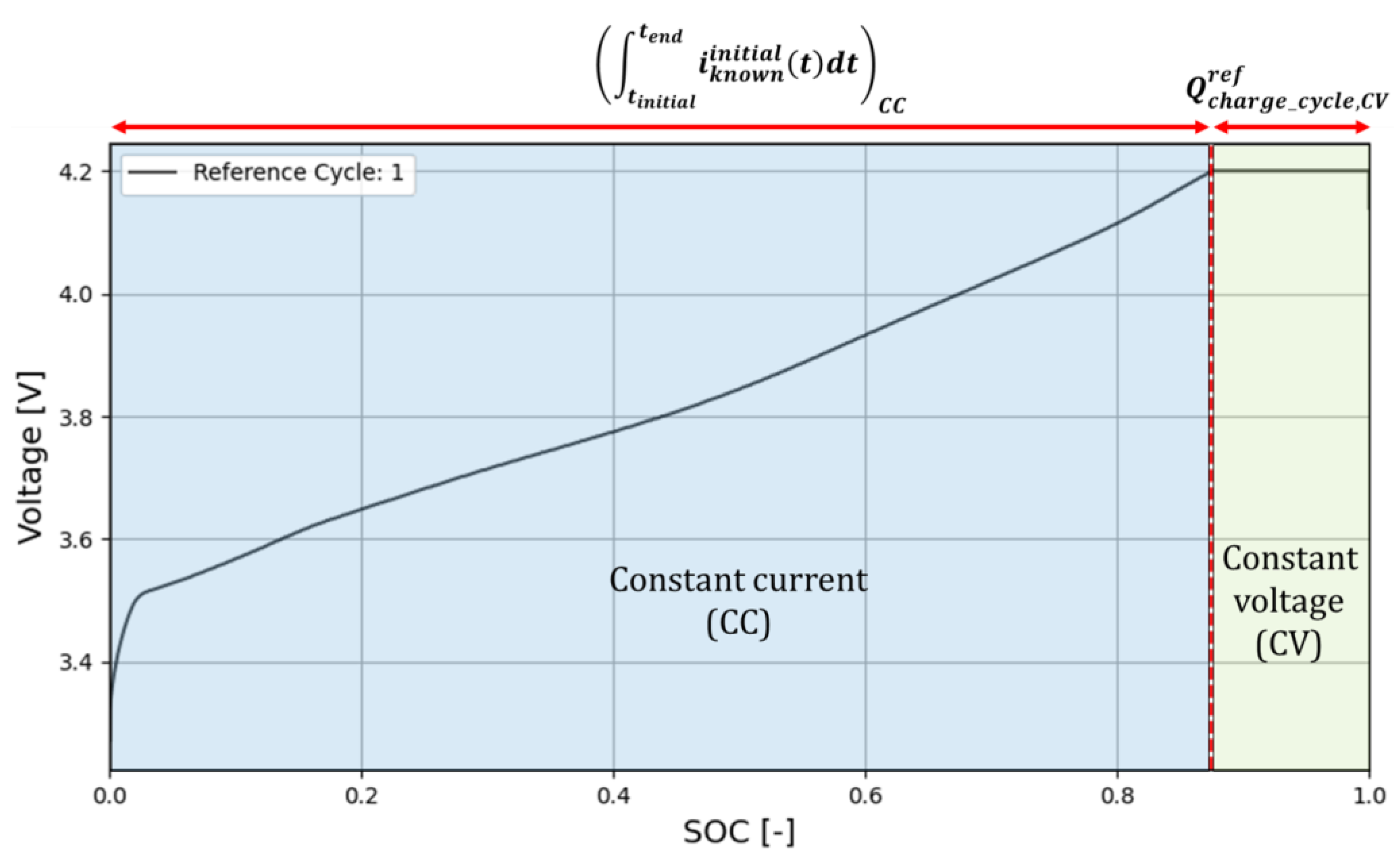
Phase 1.1. 

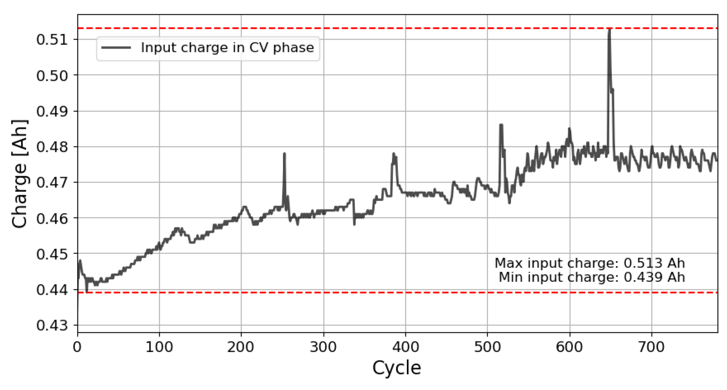
Reference charge cycle characterization. Several (SOC(t), v(t)) data points of the voltage–SOC curve of the battery are acquired, together with the input charge in the constant voltage (CV) stage of the reference charge cycle, i.e., when the battery is brand new. The initial or reference cycle determines the reference capacity of the battery.

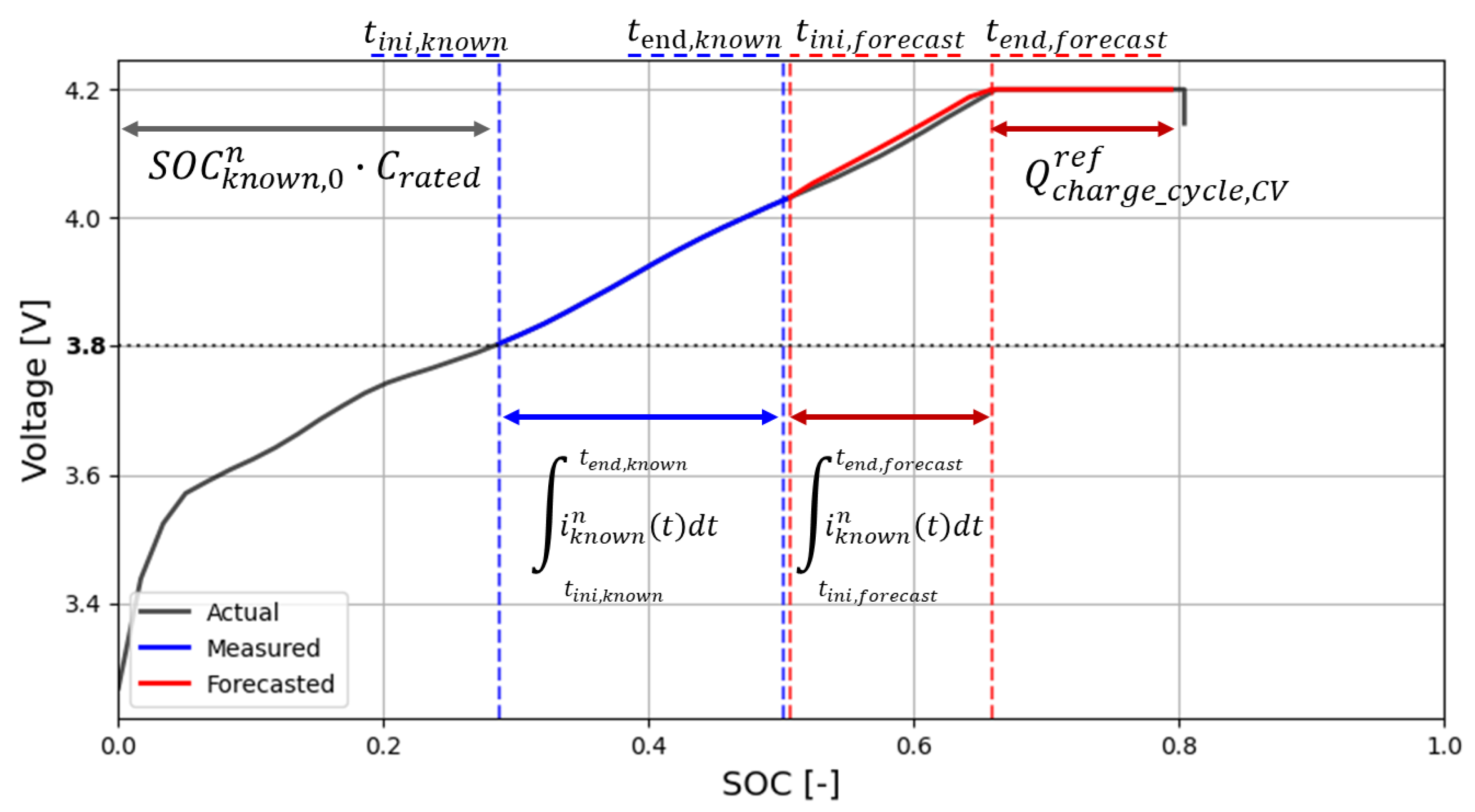
Phase 1.2. 

Nernst equation fitting and forecasting. During the constant current (CC) stage of a generic charge cycle over the lifetime of the battery, a few data points (SOC(t), v(t)) corresponding to a portion of the generic charge cycle are used to fit the Nernst equation and forecast the behavior of the voltage–SOC curve during the remaining charge period.

Phase 1.3. 

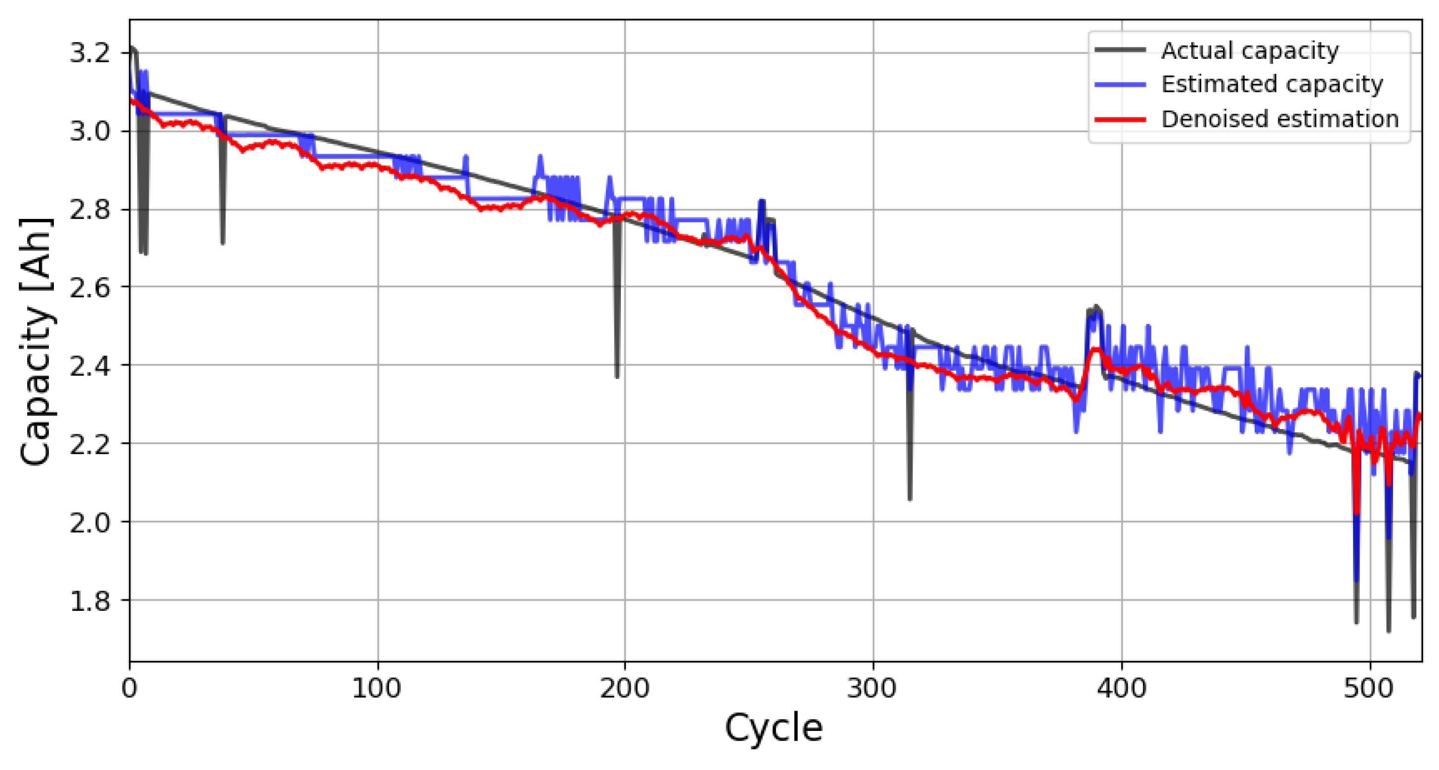
Capacity estimation. The total charge that the battery can hold in a given cycle (cycle capacity) is estimated based on the forecasted charge cycle and the reference cycle data.

Phase 2 models and forecasts the battery aging behavior by estimating the capacity fade of future cycles. It includes the following steps:

Phase 2.1. 

Phase 2.1 Capacity denoising and preprocessing. To improve the accuracy of the forecasting techniques in future steps, the time-series data of the calculated cycle capacity are denoised using a discrete wavelet filter. In this step, various algorithms are applied to preprocess the input data of the forecast models.

Phase 2.2. 

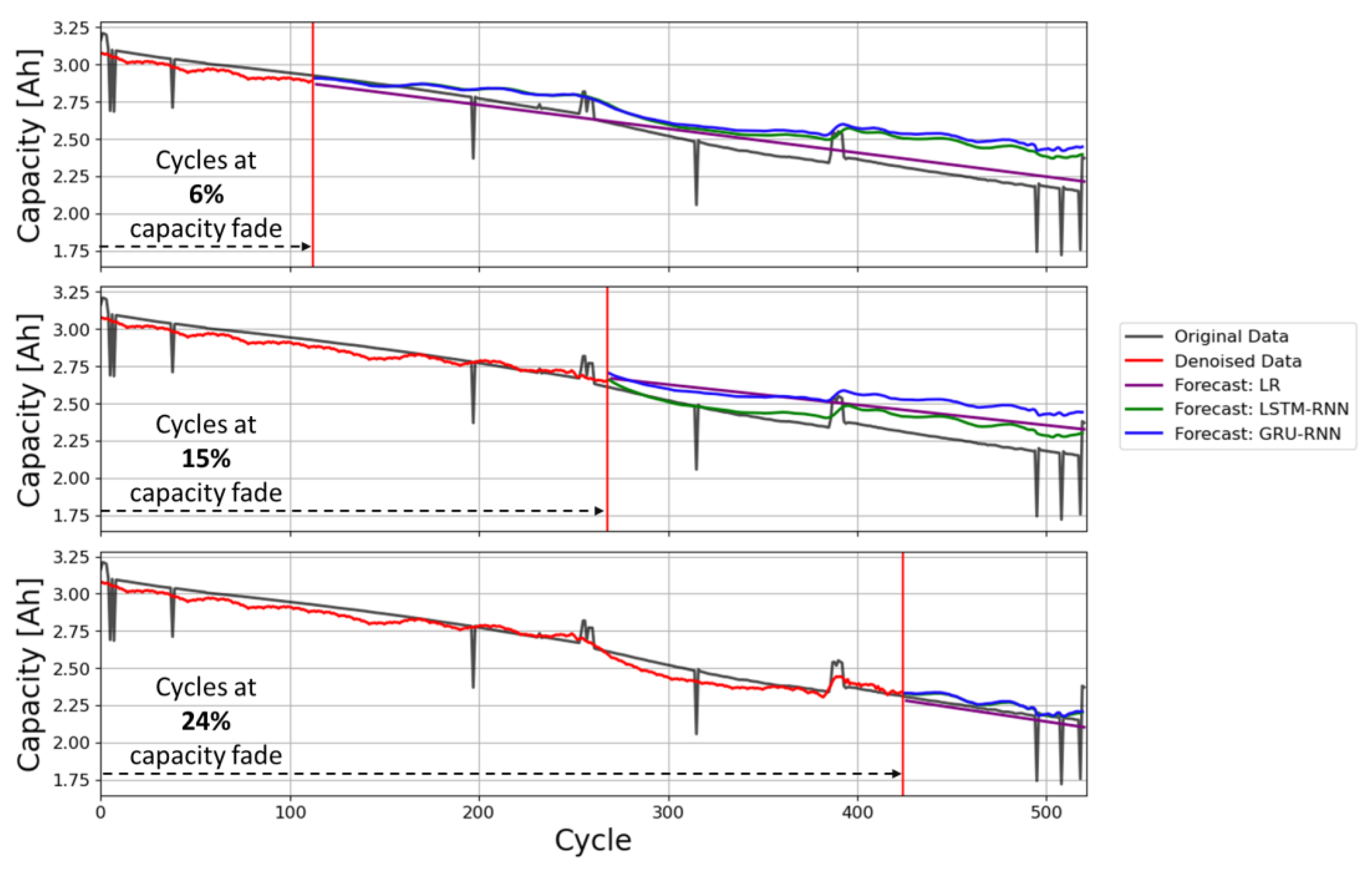
Phase 2.2 Aging behavior forecast. Using the processed data from the previous steps as input, linear regression (LR), a long short-term memory neural network (LSTM-RNN), and a gated recurrent unit neural network (GRU-RNN) are used to predict the aging behavior and degradation of the battery.

The steps described above are summarized in Figure 1.

2.1. Phase 1.1. Reference Charge Cycle Characterization

The reference cycle (cycle 1) provides relevant information for future calculations in terms of the reference capacity of the battery C^ref and the charge accumulated by the battery during the CV stage of the charge cycle $Q_{charge\_cycle,CV}^{ref}$. Note that the value of $Q_{charge\_cycle,CV}^{ref}$ remains almost constant throughout all charge cycles, regardless of the state of the battery, as shown in Section 4 (see Figure 5 and Table 2). A full discharge and a full charge are suggested to properly measure and characterize the initial or reference voltage–SOC profile of the battery.

The reference capacity C^ref of the fresh battery is calculated using the data from the initial or reference cycle as follows:

$$C^{ref}={\left({\displaystyle {\int }_{t_{initial,CC}}^{t_{end,CC}}{i}_{known}^{initial}}(t)dt\right)}_{CC}+{\left({\displaystyle {\int }_{t_{initial,CV}}^{t_{end,CV}}{i}_{known}^{initial}}(t)dt\right)}_{CV}={\left({\displaystyle {\int }_{t_{initial,CC}}^{t_{end,CC}}{i}_{known}^{initial}}(t)dt\right)}_{CC}+Q_{charge\_cycle,CV}^{ref}$$

(5)

where CC and CV refer to the constant current and constant voltage stages of the charge cycle, respectively.

Figure 2 shows the reference cycle and the different parameters in (5).

2.2. Phase 1.2. Nernst Equation Fitting and Forecast

In this work, the Nernst equation was used as a fitting tool to approximate the charge cycle using partial data from a given cycle. Assuming that the SOC is known, the cell voltage can be determined from the Nernst equation [27,28] using

$$v^{{}_n}(t)=E_0-R^{{}_n}{i}^{{}_n}(t)+{\mu }_1\ln [SOC(t)]+{\mu }_2\ln [1-SOC(t)]$$

(6)

where vⁿ(t) and iⁿ(t) are the instantaneous values of the cell voltage and current at cycle n, E₀ is the standard cell potential, Rⁿ is the internal resistance of the cell calculated at each cycle, and μ₁ and μ₂ are constant parameters. Figure 3 shows the profile of the Nernst equation.

Since the current is a constant value during the CC stage of the charge cycle, (6) can be rewritten for fitting purposes as (7), which depends only on three unknowns, namely, a, b, and c, according to

$$y(t)=a+b\ln [x(t)]+c\ln [1-x(t)]$$

(7)

where x(t) corresponds to SOC(t) and y(t) to vⁿ(t). The generalized least squares (GLS) method [29] is used to determine the values of the unknowns a, b, and c from experimental data using Equation (7).

2.3. Phase 1.3. Capacity Estimation

This study assumed that the charge cycle consisted of a constant current (CC) stage followed by a constant voltage (CV) stage because this is probably the most applied charge strategy [30]. The input charge during the CV stage in any charge cycle was assumed to be the same as that measured in the reference cycle because, as discussed in more detail in Section 4 (see Figure 5 and Table 2), this value remains relatively constant over the life of the battery.

According to the proposed method, the cycle capacity at any time of the battery’s life can be estimated with only a few points (about 20% of the entire charge cycle) taken during the interval (t_ini,known,t_end,known) of the voltage–SOC curve of the charge cycle, as shown in Figure 4. In this interval, the GLS method uses the Nernst equation to estimate the three unknowns a, b, and c. Once the fitted curve is obtained, it is used to forecast the remaining data points to the ending point of the CC stage of the charge cycle, as shown in Figure 4.

The estimated cycle capacity at cycle n can be calculated using

$$C^n=SO{C}_{known,0}^n{C}_{rated}+{\displaystyle {\int }_{t_{ini,known}}^{t_{end,known}}{i}_{known}^n}(t)dt+{\displaystyle {\int }_{t_{ini,forecast}}^{t_{end,forecast}}{i}_{known}^n}(t)dt+Q_{charge\_cycle,CV}^{ref}$$

(8)

where n stands for the nth charge cycle, Cⁿ is the estimated cycle capacity at cycle n (it is an indicator of the SOH of the battery), $SO{C}_{known,0}^n$ is the SOC value at the first point of measure in cycle n, t_ini,known and t_end,known establish the time interval where the measured values of the voltage–SOC curve are taken during the CC stage, t_ini,forecast and t_end,forecast define the time forecast interval of the voltage–SOC curve, and $Q_{charge\_cycle,CV}^{ref}$ is the total input charge during the CV stage of the reference cycle.

Note that as shown in Figure 4, this study arbitrarily chose 3.8 V as the starting point t_ini,known, while t_end,known corresponds to the time at which the SOC increased by 0.2 from t_ini,known, and thus,

SOC(t_end,known) = SOC(t_ini,known) + 0.2

(9)

Note that during the CC phase, there is a proportional relationship between the time and the SOC.

From (9), it can be deduced that only about 20% of the points of the charge cycle are necessary for the prediction of the estimated cycle capacity Cⁿ at cycle n. It is also noted that t_ini,forecast = t_end,known and t_end,forecast corresponds to the time when the battery voltage reaches 4.2 V, i.e., the starting point of the CV stage.

2.4. Phase 2.1. Capacity Denoising and Preprocessing

The evolution over the lifetime of the estimated cycle capacity Cⁿ at each cycle n contains high-frequency noise components due to the test conditions, the experimental measurements, the nonlinear behavior of the battery, and even the GLS fitting procedure; therefore, a noise-reduction stage is required. Although other filtering approaches are possible [31], a four-stage discrete wavelet transform (DWT) using a discrete Meyer mother wavelet was applied in this study because it is well suited for signal denoising in forecasting applications [32]. As shown in Appendix A, this method decomposes the signals into different frequency components, allowing for the noise they contain to be selectively eliminated, thereby improving the accuracy and reliability of predictive models.

This step also includes several sequential steps applied to the data of the denoised estimated cycle capacity, such as detrending, normalization, and formatting [33] in order to improve the performance of the capacity fade forecasting methods.

2.5. Phase 2.2. Aging Behavior Forecast

In this study, the capacity of future cycles was estimated using three methods, namely, linear regression (LR), a long short-term memory recurrent neural network (LSTM-RNN), and a gated recurrent unit recurrent neural network (GRU-RNN), to predict the aging behavior and capacity fade of the battery.

Linear regression, which is one of the most basic techniques in statistical modeling and machine learning [34], serves as a fundamental tool for modeling the relationship between a dependent variable and one or more independent variables by identifying the linear relationship that best represents the underlying pattern in the data. Its simplicity, interpretability, and computational efficiency make it particularly suitable for tasks where the underlying relationship between variables can be approximated using a linear model.

The LSTM neural network, proposed by Hochreiter and Schmidhuber in 1997 [35], is structured with three gating mechanisms, i.e., input, forget, and output gates. These gates allow LSTMs to retain or discard information over time, facilitating the learning of long-term dependencies in sequential data. The inherent ability of LSTMs to capture and store information over extended sequences has been particularly effective in time-series prediction.

Gated recurrent units (GRUs), introduced by Cho et al. in 2014 [36], represent a simplified variant of LSTMs with a reduced number of gates. The absence of a separate memory cell in GRUs results in computational efficiency and faster convergence during training. Despite their structural simplicity, GRUs show commendable effectiveness in modeling temporal dependencies, making them an attractive choice for scenarios with limited computational resources or data sets.

It should be noted that all models, data processing, and forecasting performed in this study were done using Python 3.10.9, which is a high-level general-purpose open-source programming language. All the modules used, such as NumPy, Pandas, SciPy, and Scikit-learn, which are required for the computation of the results, are also open source and public.

3. Data Description

The data of the cells investigated in this study were acquired and published by Sandia National Laboratories (SNL) [37] through the open-access web platform batteryarchive.org [38]. The data set includes data from several commercially available 18650 cells of different chemistries under different test conditions.

Table 1. Technical specifications of the Sandia National Laboratories database batteries investigated in this study and their test conditions.

Cathode Chemistry	NCA	NMC
Manufacturer	Panasonic	LG Chem
Manufacturer PN	NCR18650B	18650HG2
Battery type	18650	18650
Nominal capacity [Ah]	3.2	3
Nominal voltage [V]	3.6	3.6
Voltage range [V]	2.5 to 4.2	2 to 4.2
Max discharge current [A]	6	20
Temperature range [°C]	0 to 45	−5 to 50
Charge C-rate	0.5C	0.5C
Discharge C-rate	0.5C/1C/2C	0.5C/1C/2C
Test temperature [°C]	15 °C/25 °C/35 °C	15 °C/25 °C/35 °C
Depth of discharge	0% to 100%	0% to 100%

summarizes the analyzed cell characteristics and cycling conditions.

As shown in Table 1, this study focused on two cathode chemistries (NCA and NMC) cycled at different C-rates (0.5C during the charge cycle and different C-rates during the discharge cycle, i.e., 0.5C/1C/2C) and operated at different constant temperatures (15 °C, 25 °C, and 35 °C). The behaviors of a total of 39 cells were investigated in this study.

The tests were performed using an Arbin Instruments SCTS & Arbin high-precision battery tester (LBT21084, Arbin Instruments, College Station, TX, USA) for cycling and a thermal test chamber (T10C-1.5 SPX, Tenney, New Columbia, PA, USA) for temperature control.

4. Experimental Results

This section describes the results obtained with two cathode chemistries (NCA and NMC) of Li-ion batteries using the method described in Section 2. Note that all experimental results related to battery cycling were obtained from the Sandia National Laboratories (SNL) battery database [37] through the open-access web platform batteryarchive.org [38].

As explained in Section 2.1, the value of $Q_{charge\_cycle,CV}^{ref}$, which was calculated along the CV stage of the reference charge cycle, remained almost constant throughout all the charge cycles, regardless of the battery cycle analyzed. Figure 5 and

Table 2. Accumulated charge during the CV stage of the charge cycle over the life of the batteries. Average maximum differences for the 39 analyzed batteries of NCA and NMC cathode chemistries between the reference cycle and all cycles over the life of the batteries.

Tambient	15 °C				25 °C						35 °C
Cathode	NCA		NMC		NCA			NMC			NCA		NMC
C-Rate	1	2	1	2	0.5	1	2	0.5	1	2	1	2	1	2
Average max. difference [Ah]	0.08	0.10	0.04	0.03	0.05	0.06	0.08	0.21	0.14	0.09	0.09	0.09	0.07	0.07
Average max. difference [%] *	2.73	3.41	1.46	1.08	0.44	2.03	2.62	7.14	4.63	3.06	2.50	2.80	2.38	2.38

* Percentage of the average maximum difference referred to the reference capacity.

confirm this statement.

The results presented in Figure 5 clearly show that despite some small fluctuations, the amount of charge accumulated in the battery during the CV stage of the nth charge cycle $Q_{charge\_cycle,CV}^n$ corresponding to the plateau region of Figure 2 and Figure 4 remained almost constant throughout all the charge cycles, regardless of the battery cycle analyzed.

Table 2 summarizes the average maximum differences between the reference cycle and all cycles over the life of the batteries for the different cathode chemistries of the parameter $Q_{charge\_cycle,CV}^n$.

The results summarized in Table 2 show the small percentage differences between $Q_{charge\_cycle,CV}^n$ corresponding to the nth generic cycle and that of the reference cycle $Q_{charge\_cycle,CV}^{ref}$.

Figure 6 shows the evolution of the cycle capacity calculated from the Coulomb count (reference method) using all available experimental data over the life of the battery, the cycle capacity estimated using the GLS–Nernst approach over the life of the battery, and the denoised estimated cycle capacity.

The results presented in Figure 6 show a great similarity between the values obtained for the cycle capacity using the Coulomb counting method and those obtained with the GLS–Nernst estimation method, which is a confirmation of the usefulness and accuracy of the proposed approach.

The mean absolute percentage error between two time series is defined as

$$MAPE=\frac{100}{m}{\displaystyle \sum _{i=1}^m\left|\frac{C_{cycle\_CC,i}-C_{estimated,i}}{C_{cycle\_CC,i}}\right|}$$

(10)

where C_{cycle_CC,i} is the cycle capacity at cycle i obtained using Coulomb counting, C_estimated,i is the value obtained by denoising the GLS–Nernst estimate at the same cycle, and m is the number of samples. The root-mean-square error is defined as

$$RMSE=\sqrt{\frac{1}{m}{(C_{cycle\_CC,i}-C_{estimated,i})}^2}$$

(11)

Table 3. Average RMSE and MAPE errors between the Coulomb counting cycle capacity and the denoised estimated cycle capacity calculated for the 39 batteries analyzed over their full lifetime for CV stage starting at 3.7, 3.8, and 3.9 V.

Tambient		15 °C				25 °C						35 °C
	Cathode	NCA		NMC		NCA			NMC			NCA		NMC
V	C-Rate	1	2	1	2	0.5	1	2	0.5	1	2	1	2	1	2
3.7	RMSE	0.11	0.12	0.11	0.07	0.09	0.09	0.11	0.35	0.34	0.17	0.18	0.17	0.17	0.16
	MAPE	4.46	5.16	5.27	3.05	2.54	3.16	3.78	13.80	13.78	7.02	5.71	6.40	6.61	6.15
3.8	RMSE	0.06	0.11	0.07	0.04	0.04	0.06	0.1	0.18	0.21	0.22	0.09	0.12	0.17	0.21
	MAPE	2.23	4.08	1.81	1.4	1.34	1.75	2.77	6.26	7.23	9.05	2.18	3.86	6.69	8.23
3.9	RMSE	0.04	0.05	0.13	0.12	0.05	0.07	0.08	0.11	0.07	0.11	0.12	0.14	0.13	0.15
	MAPE	1.14	1.89	6.30	5.84	1.87	2.32	3.02	2.67	2.82	4.54	3.99	5.55	5.22	5.62

summarizes the average error values (RMSE and MAPE) for the 39 batteries analyzed with NCA and NMC cathode chemistries, as calculated between the cycle capacity of the batteries over the full life cycle and the denoised GLS–Nernst estimation of the capacity. Note that although this work suggests starting measurements on the CC phase at 3.8 V, Table 3 also shows the results starting at 3.7 V and 3.9 V to show that the method can work at different voltages and give similar results.

The results summarized in Table 3 show that the mean absolute percentage error (MAPE) of the estimated capacity of the analyzed batteries using the proposed GLS–Nernst approach was between 1.34% and 9.05% with 3.8 V as the starting voltage, which is an acceptable value that validates the method proposed in this work.

Regarding the capacity prediction results, Figure 7 shows the forecasted cycle capacities using the LR, LSTM-RNN, and GRU-RNN methods at cycles corresponding to 6%, 15%, and 24% of capacity fade with respect to the initial or reference capacity.

Table 4. Average RMSE and MAPE errors between the Coulomb counting cycle capacity and the forecasted cycle capacity calculated at cycles corresponding to 6%, 15%, and 24% of capacity fade with respect to the reference capacity. Errors averaged for the 39 batteries analyzed over their full lifetime.

Forecast Errors Calculated at the Cycle Corresponding to 6% Capacity Fade
	TAmb	15 °C				25 °C						35 °C
	Cathode	NCA		NMC		NCA			NMC			NCA		NMC
	C-Rate	1	2	1	2	0.5	1	2	0.5	1	2	1	2	1	2	Average
LR	RMSE	0.09	0.13	0.19	0.19	0.17	0.13	0.14	0.16	0.26	0.24	0.23	0.20	0.22	0.28	0.19
	MAPE	3.54	5.14	9.68	9.41	6.10	4.77	5.51	6.57	10.50	10.55	7.75	7.71	9.29	11.49	7.72
GRU	RMSE	0.48	0.80	0.29	0.27	0.05	0.28	0.38	0.75	0.40	0.30	0.15	0.31	0.34	0.15	0.35
	MAPE	19.20	40.47	13.61	10.48	1.59	9.70	15.66	28.82	15.60	10.63	4.65	11.15	12.30	5.60	14.25
LSTM	RMSE	0.08	0.15	0.17	0.11	0.10	0.08	0.11	0.14	0.24	0.24	0.16	0.16	0.20	0.27	0.16
	MAPE	3.09	5.66	8.63	5.28	3.40	2.83	3.27	5.87	9.68	10.57	4.92	5.59	8.18	11.11	6.29
Forecast Errors Calculated at the Cycle Corresponding to 15% Capacity Fade
	TAmb	15 °C				25 °C						35 °C
	Cathode	NCA		NMC		NCA			NMC			NCA		NMC
	C-Rate	1	2	1	2	0.5	1	2	0.5	1	2	1	2	1	2	Average
LR	RMSE	0.05	0.12	0.05	0.03	0.06	0.06	0.12	0.15	0.19	0.2	0.14	0.15	0.17	0.21	0.12
	MAPE	1.7	3.84	2.16	1.54	2.49	2.03	3.79	6.21	7.34	8.93	4.33	5.74	7.18	8.35	4.69
GRU	RMSE	0.24	0.3	0.28	0.32	0.1	0.21	0.12	0.18	0.12	0.33	0.15	0.41	0.14	0.1	0.21
	MAPE	10.38	13.95	14.85	15.25	3.82	8.03	4.05	7.43	4.8	14.16	4.89	17.67	5.26	3.09	9.12
LSTM	RMSE	0.04	0.15	0.06	0.02	0.03	0.07	0.12	0.14	0.16	0.21	0.12	0.15	0.15	0.19	0.12
	MAPE	1.51	5.53	2.69	0.78	0.86	2.21	3.57	5.85	6.28	9.12	3.3	5.84	6.12	7.75	4.39
Forecast Errors Calculated at the Cycle Corresponding to 24% Capacity Fade
	TAmb	15 °C				25 °C						35 °C
	Cathode	NCA		NMC		NCA			NMC			NCA		NMC
	C-Rate	1	2	1	2	0.5	1	2	0.5	1	2	1	2	1	2	Average
LR	RMSE	0.04	0.15	0.06	0.02	0.01	0.07	0.15	0.12	0.12	0.21	0.09	0.15	0.11	0.19	0.11
	MAPE	1.83	5.1	3.23	0.88	0.43	2.67	5.71	4.86	5.16	9.28	2.8	5.85	4.69	7.41	4.28
GRU	RMSE	0.09	0.24	0.06	0.17	0.05	0.13	0.13	0.13	0.08	0.2	0.1	0.21	0.09	0.17	0.13
	MAPE	3.88	12.12	3.07	8.93	1.61	5.18	2.49	5.71	3.12	9.25	3.62	8.23	3.72	6.66	5.54
LSTM	RMSE	0.05	0.17	0.08	0.02	0.02	0.06	0.15	0.12	0.11	0.22	0.08	0.17	0.12	0.2	0.11
	MAPE	2.04	6.48	4.64	0.78	0.63	2.34	4.62	5.24	4.79	9.9	2.41	7.47	4.87	7.76	4.57

summarizes the average error values (RMSE and MAPE) for the 39 batteries analyzed with NCA and NMC cathode chemistries, as calculated between the Coulomb counting cycle capacity of the batteries and the denoised CNC-LR forecasted cycle capacity over the remaining life cycle calculated at cycles corresponding to 6%, 15%, and 24% of capacity fade with respect to the reference capacity (see Figure 7).

The results presented in Table 4 show that as expected, the forecast errors for the three forecasting methods tended to decrease as more historical data (number of cycles) were available. However, there were some differences between the three forecasting methods. While LSTM clearly outperformed the other methods when there were few data available, this difference tended to decrease as the amount of data available increased.

Deep learning algorithms have been applied to the prediction of Li-ion battery degradation. However, most of the work dealt with full cycle data, such as in [39], where the degradation of NMC and LFP batteries was predicted using a deep learning framework cored by a recurrent neural network. In [40], indicators such as loss of lithium inventory (LLI) or loss of active material (LAM), which are difficult to measure, were used to predict battery degradation. The authors in [41] used data from several batteries with NCA and NMC cathodes as the input to train an LSTM-RNN model. Although the above works can achieve good mean RMSE errors, they still require full cycles of historical data to achieve their results, while this study could achieve similar error margins with only partially measured cycles.

Finally,

Table 5. Computation time for each method averaged over all batteries analyzed.

Method	Average Computation Time per Cycle [s]
Capacity estimation	0.00158
DWT denoising	0.00053
LR	0.00188
GRU	19.28116
LSTM	21.13642

summarizes the computation times of all the methods averaged over all the batteries tested using an Intel i9-13900K processor (Intel, Santa Clara, CA, USA).

5. Conclusions

Today, lithium-ion batteries are key elements in energy storage systems deployed around the world. However, due to their continuous use, cycling, load, and environmental conditions, the battery capacity, which is an indicator of the battery SOH, degrades over time. This study has addressed this issue by proposing a method to estimate the cycle capacity of the battery and its remaining lifetime. Since the battery capacity cannot be measured directly, this study developed a real-time method to estimate the battery cycle capacity using data from a short period of each charge cycle using a GLS–Nernst approach. By analyzing the historical capacity data of a battery, this study also developed a method to predict its degradation in real time based on three prediction methods, namely, LR, LSTM-RNN, and GRU-RNN. Both approaches for estimating the cycle capacity of the battery and predicting the capacity fade were tested using experimental data from 39 Li-ion batteries of two cathode chemistries operating under different test conditions. The results presented in this paper show the accuracy of both approaches and quantify the average errors, which were low enough in all cases to validate this proposal.

The proposed approach allows for assessing a battery’s state of health in real time and also offers a forward-looking perspective to determine the degradation of the battery without the need for data of a full charge cycle (from 0% SOC to 100% SOC), but using only 20% of the full charge cycle starting from any voltage above 3.8 V. These developments have potential implications for the application of predictive maintenance and management strategies of battery systems, allowing for extending the battery lifetime, which is particularly important in applications where high reliability and longevity are critical factors.

References

- Huang, Y. The discovery of cathode materials for lithium-ion batteries from the view of interdisciplinarity. Interdiscip. Mater. 2022, 1, 323–329. [Google Scholar] [CrossRef]
- Spitthoff, L.; Øyre, E.S.; Muri, H.I.; Wahl, M.; Gunnarshaug, A.F.; Pollet, B.G.; Lamb, J.J.; Burheim, O.S. Thermal management of lithium-ion batteries. In Micro-Optics and Energy: Sensors for Energy Devices; Springer: Berlin/Heidelberg, Germany, 2020; pp. 183–194. [Google Scholar]
- Meng, J.; Ricco, M.; Luo, G.; Swierczynski, M.; Stroe, D.I.; Stroe, A.I.; Teodorescu, R. An Overview and Comparison of Online Implementable SOC Estimation Methods for Lithium-Ion Battery. IEEE Trans. Ind. Appl. 2018, 54, 1583–1591. [Google Scholar] [CrossRef]
- Meng, J.; Luo, G.; Gao, F. Lithium polymer battery state-of-charge estimation based on adaptive unscented kalman filter and support vector machine. IEEE Trans. Power Electron. 2016, 31, 2226–2238. [Google Scholar] [CrossRef]
- Tao, R.; Gu, Y.; Sharma, J.; Hong, K.; Li, J. A conformal heat-drying direct ink writing 3D printing for high-performance lithium-ion batteries. Mater. Today Chem. 2023, 32, 101672. [Google Scholar] [CrossRef]
- Teodorescu, R.; Sui, X.; Vilsen, S.B.; Bharadwaj, P.; Kulkarni, A.; Stroe, D.I. Smart Battery Technology for Lifetime Improvement. Batteries 2022, 8, 169. [Google Scholar] [CrossRef]
- Zhu, J.; Xu, W.; Knapp, M.; Dewi Darma, M.S.; Mereacre, L.; Su, P.; Hua, W.; Liu-Théato, X.; Dai, H.; Wei, X.; et al. A method to prolong lithium-ion battery life during the full life cycle. Cell Reports Phys. Sci. 2023, 4, 101464. [Google Scholar] [CrossRef]
- Ruan, H.; Barreras, J.V.; Engstrom, T.; Merla, Y.; Millar, R.; Wu, B. Lithium-ion battery lifetime extension: A review of derating methods. J. Power Sources 2023, 563, 232805. [Google Scholar] [CrossRef]
- Jin, S.; Huang, X.; Sui, X.; Wang, S.; Teodorescu, R.; Stroe, D.I. Overview of Methods for Battery Lifetime Extension. In Proceedings of the 2021 23rd European Conference on Power Electronics and Applications (EPE’21 ECCE Europe), Ghent, Belgium, 6–10 September 2021. [Google Scholar]
- Harper, G.; Sommerville, R.; Kendrick, E.; Driscoll, L.; Slater, P.; Stolkin, R.; Walton, A.; Christensen, P.; Heidrich, O.; Lambert, S.; et al. Recycling lithium-ion batteries from electric vehicles. Nature 2019, 575, 75–86. [Google Scholar] [CrossRef]
- Woody, M.; Arbabzadeh, M.; Lewis, G.M.; Keoleian, G.A.; Stefanopoulou, A. Strategies to limit degradation and maximize Li-ion battery service lifetime—Critical review and guidance for stakeholders. J. Energy Storage 2020, 28, 101231. [Google Scholar] [CrossRef]
- Chung, C.H.; Jangra, S.; Lai, Q.; Lin, X. Optimization of Electric Vehicle Charging for Battery Maintenance and Degradation Management. IEEE Trans. Transp. Electrif. 2020, 6, 958–969. [Google Scholar] [CrossRef]
- Shen, L.; Li, J.; Meng, L.; Zhu, L.; Shen, H.T. Transfer Learning-based State of Charge and State of Health Estimation for Li-ion Batteries: A Review. IEEE Trans. Transp. 2023. [Google Scholar] [CrossRef]
- Koleti, U.R. Fast Charging Strategies in Lithium-Ion Batteries: Detection and Control of Lithium Plating; University of Warwick: Coventry, UK, 2020. [Google Scholar]
- de la Vega, J.; Riba, J.R.; Ortega-Redondo, J.A. Mathematical Modeling of Battery Degradation Based on Direct Measurements and Signal Processing Methods. Appl. Sci. 2023, 13, 4938. [Google Scholar] [CrossRef]
- Wenzl, H. BATTERIES|Capacity. In Encyclopedia of Electrochemical Power Sources; Newnes: Sebastopol, CA, USA, 2009; pp. 395–400. [Google Scholar]
- Peng, J.; Meng, J.; Chen, D.; Liu, H.; Hao, S.; Sui, X.; Du, X. A Review of Lithium-Ion Battery Capacity Estimation Methods for Onboard Battery Management Systems: Recent Progress and Perspectives. Batteries 2022, 8, 229. [Google Scholar] [CrossRef]
- Jiang, J.; Zhang, C. Fundamentals and Application of Lithium-Ion Batteries in Electric Drive Vehicles; Sons, J.W., Ed.; Wiley: Singapore, 2015. [Google Scholar]
- IEC IEC 62660-2:2018; Secondary Lithium-Ion Cells for the Propulsion of Electric Road Vehicles—Part 2: Reliability and Abuse Testing. International Electrotechnical Commission: Geneva, Switzerland, 2018.
- ISO ISO 6469-1:2019; Electrically Propelled Road Vehicles—Safety Specifications—Part 1: Rechargeable Energy Storage System (RESS). ISO: Geneva, Switzerland, 2019.
- IEEE IEEE Std 450-2020; Recommended Practice for Maintenance, Testing, and Replacement of Vented Lead-Acid Batteries for Stationary Applications. IEEE: Piscataway Township, NJ, USA, 2020.
- Meng, J.; Cai, L.; Luo, G.; Stroe, D.I.; Teodorescu, R. Lithium-ion battery state of health estimation with short-term current pulse test and support vector machine. Microelectron. Reliab. 2018, 88–90, 1216–1220. [Google Scholar] [CrossRef]
- Song, Y.; Li, L.; Peng, Y.; Liu, D. Lithium-Ion Battery Remaining Useful Life Prediction Based on GRU-RNN. In Proceedings of the 2018 12th International Conference on Reliability, Maintainability, and Safety (ICRMS), Shanghai, China, 17–19 October 2018; pp. 317–322. [Google Scholar]
- Park, K.; Choi, Y.; Choi, W.J.; Ryu, H.Y.; Kim, H. LSTM-Based Battery Remaining Useful Life Prediction with Multi-Channel Charging Profiles. IEEE Access 2020, 8, 20786–20798. [Google Scholar] [CrossRef]
- Zhao, J.; Zhu, Y.; Zhang, B.; Liu, M.; Wang, J.; Liu, C.; Hao, X.; Kowal, J.; Zhao, J.; Zhu, Y.; et al. Review of State Estimation and Remaining Useful Life Prediction Methods for Lithium–Ion Batteries. Sustainability 2023, 15, 5014. [Google Scholar]
- MaximIntegrated. MAX1726x ModelGauge m5 EZ User Guide; MaximIntegrated: San Jose, CA, USA, 2018. [Google Scholar]
- Plett, G.L. Extended Kalman filtering for battery management systems of LiPB-based HEV battery packs: Part 2. Modeling and identification. J. Power Sources 2004, 134, 262–276. [Google Scholar] [CrossRef]
- Hussein, A.A.H.; Batarseh, I. An overview of generic battery models. In Proceedings of the 2011 IEEE Power and Energy Society General Meeting, Detroit, MI, USA, 24–28 July 2011. [Google Scholar]
- Wang, Y.; Meng, D.; Chang, Y.; Zhou, Y.; Li, R.; Zhang, X. Research on online parameter identification and SOC estimation methods of lithium-ion battery model based on a robustness analysis. Int. J. Energy Res. 2021, 45, 21234–21253. [Google Scholar] [CrossRef]
- Pavković, D.; Kasać, J.; Krznar, M.; Cipek, M. Adaptive Constant-Current/Constant-Voltage Charging of a Battery Cell Based on Cell Open-Circuit Voltage Estimation. World Electr. Veh. J. 2023, 14, 155. [Google Scholar] [CrossRef]
- Meng, J.; Azib, T.; Yue, M. Early-Stage end-of-Life prediction of lithium-Ion battery using empirical mode decomposition and particle filter. Proc. Inst. Mech. Eng. Part A J. Power Energy 2023. [Google Scholar] [CrossRef]
- Wang, X.; Xu, J.; Zhao, Y. Wavelet Based Denoising for the Estimation of the State of Charge for Lithium-Ion Batteries. Energies 2018, 11, 1144. [Google Scholar] [CrossRef]
- Dogan, A.; Cidem Dogan, D. A Review on Machine Learning Models in Forecasting of Virtual Power Plant Uncertainties. Arch. Comput. Methods Eng. 2023, 30, 2081–2103. [Google Scholar] [CrossRef]
- Kwon, S.J.; Han, D.; Choi, J.H.; Lim, J.H.; Lee, S.E.; Kim, J. Remaining-useful-life prediction via multiple linear regression and recurrent neural network reflecting degradation information of 20Ah LiNixMnyCo1−x−yO2 pouch cell. J. Electroanal. Chem. 2020, 858, 113729. [Google Scholar] [CrossRef]
- Hochreiter, S.; Schmidhuber, J. Long Short-Term Memory. Neural Comput. 1997, 9, 1735–1780. [Google Scholar] [CrossRef] [PubMed]
- Cho, K.; van Merriënboer, B.; Bahdanau, D.; Bengio, Y. On the Properties of Neural Machine Translation: Encoder-Decoder Approaches. arXiv 2014, arXiv:1409.1259. [Google Scholar]
- Preger, Y.; Barkholtz, H.M.; Fresquez, A.; Campbell, D.L.; Juba, B.W.; Romàn-Kustas, J.; Ferreira, S.R.; Chalamala, B. Degradation of Commercial Lithium-Ion Cells as a Function of Chemistry and Cycling Conditions. J. Electrochem. Soc. 2020, 167, 120532. [Google Scholar] [CrossRef]
- Available online: https://www.batteryarchive.org/ (accessed on 27 November 2023).
- Lu, J.; Xiong, R.; Tian, J.; Wang, C.; Hsu, C.W.; Tsou, N.T.; Sun, F.; Li, J. Battery degradation prediction against uncertain future conditions with recurrent neural network enabled deep learning. Energy Storage Mater. 2022, 50, 139–151. [Google Scholar] [CrossRef]
- Costa, N.; Sánchez, L.; Anseán, D.; Dubarry, M. Li-ion battery degradation modes diagnosis via Convolutional Neural Networks. J. Energy Storage 2022, 55, 105558. [Google Scholar] [CrossRef]
- Wang, Y.; Zhu, J.; Cao, L.; Gopaluni, B.; Cao, Y. Long Short-Term Memory Network with Transfer Learning for Lithium-ion Battery Capacity Fade and Cycle Life Prediction. Appl. Energy 2023, 350, 121660. [Google Scholar] [CrossRef]
- Lee, G.R.; Gommers, R.; Waselewski, F.; Wohlfahrt, K.; O’Leary, A. PyWavelets: A Python package for wavelet analysis. J. Open Source Softw. 2019, 4, 1237. [Google Scholar] [CrossRef]
- Matlab Introduction to Wavelet Families. Available online: https://www.mathworks.com/help/wavelet/gs/introduction-to-the-wavelet-families.html (accessed on 17 December 2023).