Abstract
The conventional ultrasonic thickness measurement method is ineffective in detecting the measured specimen with a step change in thickness as it is easy to cause multimode acoustic mixing in the ultrasonic detection process. To solve this problem, this paper presented an electromagnetic acoustic resonance (EMAR) moving scan identification method based on a frequency–frequency energy density precipitation (FFEDP) algorithm, which uses a standing wave resonance mode to accurately extract step thickness information and employs the algorithm to separate step thickness information. According to the simulation results, the ratio of the highest energy density of the spectrum signal on both sides of the step area to the total energy density had an opposite linear change rule with the equidistant movement of the transducer coil. The thickness step area can be identified by analyzing the crossover point of the contrast value change. The experimental results showed that the proposed method can accurately extract the thickness information under millimeter-level stepping distance for sector-notched specimens with step surfaces of different thicknesses, and at the same time realize the effective identification of the step surface.
1. Introduction
Because of their unique performance advantages, aluminum–magnesium alloy sheets are widely used in the industrial manufacturing, aerospace, and petrochemical industries, as well as other industries around the world [1]. In practical engineering applications, the material thickness may gradually change because of nonuniform embossing, wear, and media corrosion in operating environments. This would affect the strength and stiffness of metal structures and even compromise the safety of equipment operation. To estimate the remaining service life, it is crucial to evaluate the state of thickness development [2,3].
Compared with other classical non-destructive testing methods, ultrasonic testing (UT) technology is considered one of the most promising technologies for thickness measurement and has been extensively researched and applied in the field of monitoring the thickness profile of sheet metal. Most conventional ultrasonic thickness measurement techniques use piezoelectric ultrasonic transducers, which have significant application limitations because they require coupling agents to transmit the ultrasound generated by the piezoelectric chip into the specimen under the influence of an electrical pulse [4,5]. As a non-contact detection technique, electromagnetic ultrasound detection technology [6,7,8] generates ultrasound directly within the skin depth of the measured object under the influence of electromagnetic coupling, not requiring pretreating the surface, and can detect under high temperatures, high pressures, and other complicated on-site environments. Kim et al. [9] used EMAT to demonstrate the ability of guided wave signals to effectively evaluate changes in aluminum plate thickness caused by corrosion and friction. Parra-Raad et al. [10] also realized effective detection of aluminum block thickness by using ultrasonic shear waves. However, the ultimate detection accuracy will be partially impacted by the low spatial resolution of EMAT and the low signal-to-noise ratio of receiving and retrieving waves, which are caused by the limitations of energy conversion efficiency [11,12,13]. EMAR technology has garnered a lot of interest as a potential solution to this issue.
EMAR technology is a non-destructive testing method based on electromagnetic ultrasonic transducers, which can improve the efficiency of electromagnetic weak coupling by exciting long-period signals to cause the acoustic waves to resonate [14,15,16]. Diguet et al. [17] used EMAR to prove the feasibility of accurate thickness measurement on carbon steel plates corroded in an acid solution. Yusa et al. [18] employed the EMAR approach to quantify the thickness of acid-etched metal rough interview sections, provided a new data fitting scheme and probability of detection (POD) model, and demonstrated the model’s capacity to characterize thin metal by setting various thresholds. Liu et al. [19] effectively improved the spatial resolution in the range of sound field and the detection ability of small defects by using an electromagnetic acoustic transducer composed of small magnets in the EMAR mode. Li et al. [20] successfully measured the thickness of inclined metal plate specimens and accurately determined the inclined direction of slope specimens by using EMAR technology and the n-wave compression and multiplication technique. The aforementioned research confirms that EMAR technology has been successfully employed in thickness monitoring and may effectively limit the interference of noise signals on the detection results, enabling precise measurement.
However, present research in the field of metal thickness measurement is mostly focused on improving the detection accuracy of single thickness, and research into employing EMAR technology to detect metal plate specimens with internal thickness step change is still in its early stages. A mixture of different thickness information will be present at the transducer’s sound field interface when the material thickness changes stepwise. Conventional ultrasonic techniques cannot currently be utilized to determine which sound field the thickness has a step change in. Therefore, this paper presented a moving scan identification method of EMAR based on the FFEDP algorithm. Firstly, step thickness in multi-thickness aliasing spectrum data was accurately extracted and effectively separated using the FFEDP algorithm. The effective identification and characterization of the step surface were then accomplished by using the moving scanning method to determine the energy density ratio (EDR) variation of step thickness under various acoustic field locations of the transducer.
2. Theory and Methods
2.1. Principle of EMAR Detection
Electromagnetic ultrasonic testing is a method that uses a coil to generate a high-frequency alternating current that then generates an ultrasonic signal in the material and calculates the thickness of the tested object based on the time of flight (TOF) of the echo signal [21]. The thickness information in the echo signal will be multiplexed if the test piece’s thickness is not a constant value. At this moment, the TOF approach cannot be used to correctly measure the thickness of the specimen, so the time domain signal must be converted to the frequency domain for further processing.
When EMAT detection is adopted, EMAT (shear wave) emission is stimulated by the RF excitation voltage with carrier frequency f excited by the excitation source. The same EMAT receives the ultrasonic pulse as it passes through the specimen multiple times before its energy is completely consumed. The obtained time domain signal F(t) is shown in Figure 1, where F1(t), F2(t), …, FN(t), respectively, represent shear wave time-domain signals received by the Nth EMAT, and the expression is given as follows [22,23]:
where Ai and Φi, respectively, represent the envelope and phase of the ith time domain signal; Φ1 represents the initial phase of the excitation signal; c represents the propagation speed of the sound wave in the tested part; f represents the excitation frequency; and d represents the thickness of the tested part.
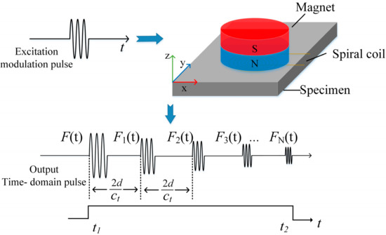
Figure 1.
Time-domain waveform diagram of EMAR.
Because of EMAT’s low energy conversion efficiency and the enormous quantity of received time domain signals Fi(t), superheterodyne phase-sensitive detection technology should be utilized for signal processing. This method combines the signal while maintaining the original signal’s phase, shifting the received signal’s carrier frequency to the intermediate frequency (IF). Next, it integrates two IF reference signals with a 90° phase difference by lining up the RF phase-sensitive detection multiplication circuit, allowing the two signal components to be acquired as follows [22,23]:
where t1 and t2 are the starting and ending time defined by the integration gate, r is the integration rate, and g is the total gain and conversion efficiency parameters. The acoustic amplitude A can be obtained by summing the two signal components:
The incident wave and the reflected wave will resonate in the specimen when the thickness d of the tested section is an exact integer multiple of the ultrasonic wave wavelength. Multiple resonant frequencies exist under frequency stimulation of a certain breadth, and the Mth resonant frequency fm and the resonant interval Δf may be represented as follows:
Therefore, the thickness of the specimen d can be obtained when the ultrasonic wave velocity c is known.
2.2. FFEDP Algorithm Theory
This paper used the FFEDP algorithm to process the multi-thickness mixing signals identified by EMAR, which is based on the time–frequency analysis principle. The method detects the thickness of the sample to acquire the standard resonance peak information of the spectrum signal, and then extracts and pre-separates the spectrum signals with varied thickness information. Following that, the continuous wavelet transformation (CWT) is applied to calculate the second time–frequency of various spectral signals to provide the corresponding energy density distribution maps and distribution curves. Finally, the EDR of signals with different thicknesses was analyzed to realize the recognition and visualization of the step surface. The following are the precise guidelines and actions:
- (1)
- The frequency domain signal obtained by frequency scanning is defined as x(m), where m = 1, 2, …, M, M is a positive integer, and the frequency coordinate is fi (i = 1,2, …, M). The height threshold and interval threshold are set when extracting the maximum point to filter the noise signal;
- (2)
- Traverse all discrete frequency points fi obtained in step (1), extract maximum points meeting the requirements, and record their frequency values in frequency coordinates;
- (3)
- Judge whether all the frequency values corresponding to the resonant maximum point are obtained. If so, continue to step (4); if not, consider the frequency coordinate fi+1 and return to step (2);
- (4)
- Ensure that there are equal gaps between each frequency value in the record. If they are equal, it means that x(m) only contains information about one thickness; therefore, move on to step (6). If they differ, it means that x(m) contains information on two or more thicknesses; continue to step (5);
- (5)
- After extraction, the frequency values at the resonant sites are compared to those of standard specimens with specified thicknesses, and the resonant peak points belonging to various thicknesses are then separated;
- (6)
- Reconstruct the signal between the two groups of resonance maximum points that were previously separated, and define the separated frequency domain signal corresponding to the various thicknesses as yh (m), where h denotes the sequential number of various thicknesses;
- (7)
- Perform CWT to the decoupled signal yh from the previous step. The frequency of the decoupled signal is represented by the ordinate Fk (k = 1, 2, …, N), where N is a positive integer, and the abscissa fi (i = 1, 2, …, M) is produced from the transform, where M is a positive integer. E(fi, Fk) is the definition of the energy density at a collection of frequency points and F-Frequency points (fi, Fk) that have been confirmed. The CWT result of the frequency domain signal yh (m) can be expressed as follows [24]:
- (8)
- For the F-Frequency energy density distribution data obtained in (7), the maximum F-Frequency energy density corresponding to each F-Frequency point Fk is extracted, and the distribution curve is drawn by fitting. According to the EMAR principle, the signal has the maximum F-Frequency energy density at 1/Δfh, and the reciprocal of the maximum value is the frequency interval Δf of the resonant spectrum of the original thickness;
- (9)
- Calculations are performed to determine the EDR on either side of the step surface, and the step surface is determined by examining the change in the proportion result.
The abovementioned are the theoretical steps of the FFEDP algorithm proposed in this paper, and its algorithm flow chart is shown in Figure 2.
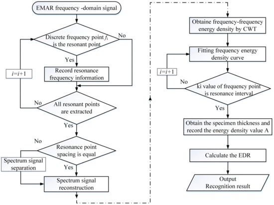
Figure 2.
EMAR step surface information separation and recognition method based on FFEDP.
3. Finite Element Simulation Analysis
Figure 3 demonstrates the electromagnetic ultrasonic testing model for step specimen components developed by COMSOL Multiphysics, which includes structural field, alternating magnetic field, static magnetic field, and other multi-physical field couplings. It is made up of the air domain, the step specimen, and the coil-producing pulsed eddy current. The dimension of the permanent magnet is 20 mm by 6 mm, and its magnetic field strength is 1.2 T. The specimen is made of 7075 aluminum alloy and has a width of 30 mm and two portions that are 6 mm and 10 mm thick, respectively. The spiral coil is made up of 28 wires. A single wire has a coil of 0.2 mm, a height of 0.3 mm, and a d-spacing of 0.1 mm between consecutive wires. The lifting distance between the permanent magnet and the coil is 0.8 mm, and the lifting distance between the coil and the specimen is 0.3 mm. The center of the wire group is located at the thickness step surface. The finite element model uses a 2D framework rather than a 3D one, which can significantly reduce the number of calculations needed to solve problems and speed up computation.
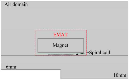
Figure 3.
2D simulation model of the step specimen.
Because the EMAR method was used to detect the specimen in this section, the frequency domain solver was used to solve the ultrasonic displacement distribution, and the frequency range was 2~4 MHz. The distribution of ultrasonic displacement at the random selection value f = 3.26 MHz when the excitation frequency did not satisfy the resonance criterion is shown in Figure 4. Figure 4a demonstrates that when the spiral coil’s center was at the point where the step’s thicknesses overlapped (that is, when the length of the coil on the 6 mm side equals the length of the coil on the 10 mm side), the spiral coil can be compared to two sound field sources for practical purposes since the current flowing through both sides of the coil was the same and flowed in the opposite direction. As a result, an ultrasonic wave with the opposite phase were generated. The ultrasonic wavelength that corresponds to each excitation frequency varied as well, yet sound waves always propagated with the same properties. However, when the central position of the spiral coil was not at the junction of the thickness of the step surface (random selection of coil area on both sides accounts for 30% and 70%), as is the case in Figure 4b, the specimen produced three kinds of ultrasonic signals since the spiral coil may now be compared to the combined activity of three acoustic field sources. For now, the analysis of ultrasonic spectrum signals stimulated by sound field source 1 could still be used to determine the thickness value of the side with a 6 mm thickness, but the spectrum data for the side with a 10 mm thickness should be obtained from the superposition of the spectrum signals of sound field sources 2 and 3. As a result, various signal processing techniques should be used depending on the transducer’s real position.
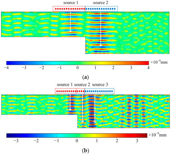
Figure 4.
Non-resonant sound field diagram of transducer at f = 3.26 MHz. (a) Ultrasonic displacement distribution when coil group is located in the center. (b) Ultrasonic displacement distribution when coil area on both sides accounts for 30% and 70%.
Additionally, the EMAR principle predicts that under frequency excitation with a specific width, there will be several resonant frequencies. When the coils were located at the center of the step surface, the frequencies f1 = 3.45 MHz and f2 = 3.35 MHz that satisfy the resonant criteria were randomly chosen, respectively. Their displacement is shown in Figure 5a,b. Since f1 and f2 are the resonant frequencies corresponding to the two thickness values respectively, the stimulated shear wave and reflected echo produced significant resonance and synergistic enhancement on the corresponding thickness side. By splitting the sweep signal, the separate spectrum signal of each thickness side can be obtained, and then the corresponding thickness value can be solved.
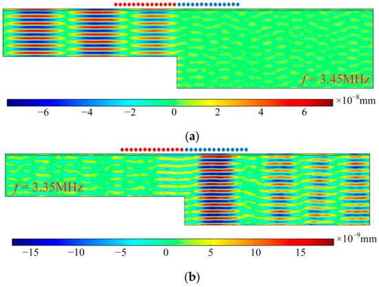
Figure 5.
Resonant displacement diagram when coil group is located in the center. (a) Diagram of resonance on the 6 mm side at f = 3.45 MHz. (b) Diagram of resonance on the 10 mm side at f = 3.35 MHz.
3.1. Method of Extracting Resonance Signals
As the two-field source model is a special case of the three-field source model, take the model shown in Figure 5b as an example, select a 2D section at the center of the coil at the side of each sound field source, and its length is equal to the thickness of the test piece, as shown in Figure 6. The spectrum analysis diagram at each thickness side of the specimen can be obtained by calculating the maximum peak value of the point displacement curve at each frequency of the three 2D transversals within the sweep frequency range, and the pre-separation of the spectrum signals with different thicknesses can then be finished. Figure 7 shows the specific computation flow diagram.
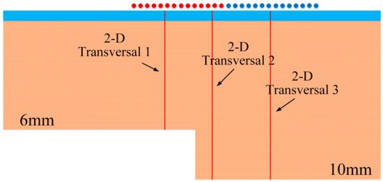
Figure 6.
Schematic diagram of 2D transversal selection.
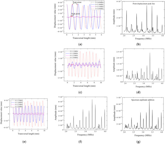
Figure 7.
Schematic of the calculating procedure for the spectrum curve. (a) Displacement curve on transversal 1. (b) Transversal 1 spectrum diagram. (c) Displacement curve on transversal 2. (d) Transversal 2 spectrum diagram. (e) Displacement curve on transversal 3. (f) Transversal 3 spectrum diagram. (g) Figure 7d,f additive spectrum diagram.
When various frequencies are excited in the sweep range, the point displacement amplitude curve on the corresponding 6 mm side 2D transversal 1 is shown in Figure 7a,b. The comparison shows that the non-resonant frequency’s point displacement amplitude was much smaller than that of the resonant frequency. The resonant spectrum diagram in the appropriate range can be created by joining the peak of the highest point displacement at each frequency. When processing the data of the 10 mm thick side, the frequency sweep result was produced by the superposition of two sound field sources, so it is essential to first obtain the spectral curves of the 2D transversals 2 and 3, then combine them to produce the final result, as shown in Figure 7c–g. The peak frequency only appeared at each resonant frequency for specimens with a single thickness, and the non-resonant frequency had a small amplitude. In this case, the resonant peak value was easily recognizable, making it simple to calculate the frequency interval Δf. When the EMAR coil group was positioned at the step specimen’s thickness step surface, the resonance interval Δf values in the spectrum analysis diagram of each thickness side that were produced by dividing the spectrum data from the frequency sweep were not identical. The signals must be further processed because it is impossible to calculate the thickness values in this case.
Then, under the proposed FFEDP algorithm’s theoretical steps, the spectrum data from the finite element simulation were first calculated. Taking 6 mm thickness side data as an example, the F-Frequency energy density distribution result calculated by CWT change is shown in Figure 8a. The figure shows that the energy of the spectrum signal was primarily centered around 4 MHz. The frequency energy density curve can be obtained by extracting the highest amplitude point corresponding to each frequency of the longitudinal frequency axis and fitting it.
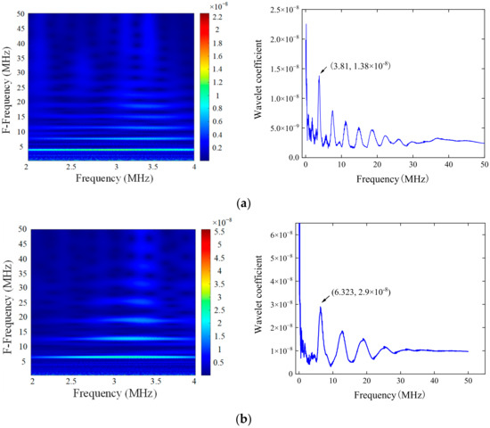
Figure 8.
F-Frequency energy density precipitation results of different thicknesses. (a) F—Frequency analysis diagram of 6 mm thickness. (b) F—Frequency analysis diagram of 10 mm thickness.
On the 6 mm thick side, the frequency where the maximum spectral energy density was located was 3.81 MHz. Because Δf is the adjacent peak difference of the original spectrum, comparable to cycle Δf, it had a frequency of 1/Δf. Therefore, 1/Δf was the outcome after the alteration. Therefore, the reciprocal of the maximum energy density was the frequency interval of the original resonance spectrum Δf. At this point, the estimated frequency interval complied with the real requirements if it roughly matched the theoretical frequency interval of the appropriate thickness value. Based on this and Formula (6), the exact thickness value could be computed to be 5.9985 mm with a mere 0.025% inaccuracy. The genuine calculation result of the 10 mm side using the same procedure was 9.96 mm with a 0.4% error, which is an accurate measurement result.
3.2. Moving Thickness Step Surface Scanning Method
For the step specimen with a thickness step surface, the propagation route of the ultrasonic wave generated by EMAR was affected not only by the relative distance between the coil and the bottom of the specimen, but also by the coil position. The excitation range of the coil’s acoustic wave varied when the position of the coil on the thickness side changed as well. As a result, the spectrum results from the frequency sweep also changed. To investigate the effect of spiral coil position on thickness detection results at the thickness step surface of the step specimen, based on the step specimen simulation model created in Section 3.1, the coil was moved 10% of the entire width of the coil from the small thickness side to the large thickness side each time until the coil was completely placed at the large thickness side, as shown in Figure 9.
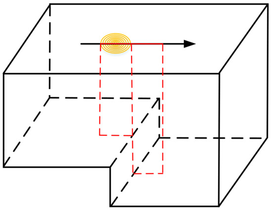
Figure 9.
Relative position of transducer coil and step surface.
As the coil moving distance increased, the area of the coil covering the tiny thickness side (that is, the area percentage of the coil covering the initial thickness side, APCIT) decreased and the area covering the opposite side increased. All test results were processed by the FFEDP algorithm, and the maximum energy density value obtained is shown in Figure 10. The figure illustrates how each thickness side’s maximum energy density values exhibited monotonic fluctuations with some regularity. To comprehend this result, the maximum energy density values for the small thickness side and large thickness side are defined as a1 and a2, respectively. Then, A1 is the EDR of the single thickness side to the total energy density, and its calculation equation is as follows:
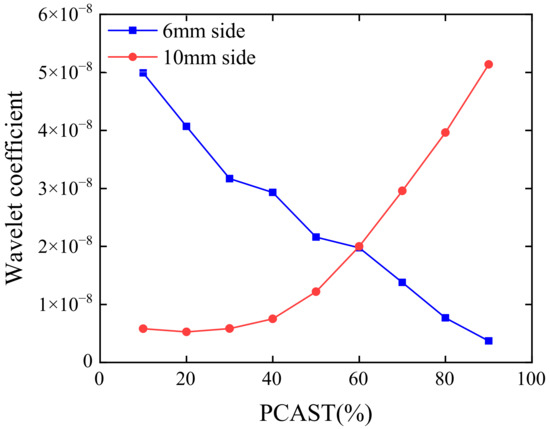
Figure 10.
Change diagram of energy density curve.
The energy density data of the 6 mm and 10 mm sides shown in Figure 10 were processed under the abovementioned approach, and the results of the EDR are displayed in Table 1. A6 gradually dropped to 0 as the spiral coil moved evenly to the right, and A10 will gradually rose to 1 as the spiral coil moved evenly to the left.

Table 1.
EDR results of transducer at different moving distances.
The amplitude quantization distribution obtained from the abovementioned EDR results is shown in Figure 11. The figure shows that as the detecting coil’s position hanged, there were clear variances in the quantization amplitude that corresponded to its EDR result. When the coil moved 60%, the color changed to a shade between green and blue, indicating a large switch in the energy percentage, which caused the thickness interface to become visible. Therefore, the visual identification and characterization of the thickness step surface can be effectively realized using this method.
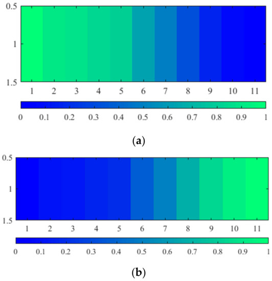
Figure 11.
Quantitative distribution diagram of energy density: (a) 6 mm side amplitude quantization distribution diagram; (b) 10 mm side amplitude quantization distribution diagram.
4. Experimental Results and Analysis
4.1. Experimental Platform
The electromagnetic ultrasonic testing system used in the experiment is shown in Figure 12. The ultrasonic wave used for detection was excited on the surface of the specimen by the high-power alternating current excited by SNAP-5000. The echo signal was then picked up by the same EMAT transducer, and ultimately the data were examined and processed by the oscilloscope.
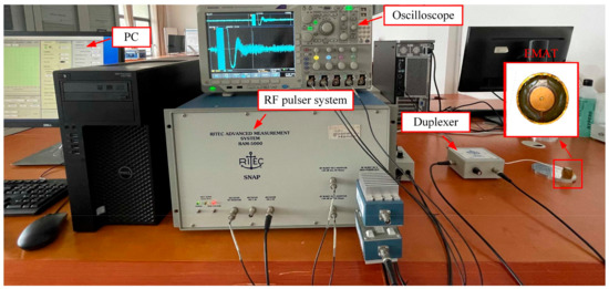
Figure 12.
Experimental system diagram.
Among them, the material of the specimen was 7075 aluminum, and all samples had sector defects at different angles at the bottom, as shown in Figure 13. Each piece that was examined had a diameter of 10 cm, a large thickness value of h1, and a small thickness value of h2. Table 2 lists the particular parameters. The transducer used in the experiment had a spiral coil construction with a 10 mm diameter. The ultrasonic testing of the circular step specimen was performed using the rotational scanning method to investigate the influence of the thickness step surface on the EMAR thickness measuring findings of the circular step specimen. To facilitate measurement, the specimen must be divided in advance, beginning with the diameter of the center line of the fan-shaped opening angle and considering the 15° rotation angle as the step length; the specimen was divided into 24 parts according to the equal angle counterclockwise, and each part was tested independently.
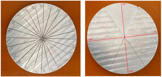
Figure 13.
Diagram of the circular step specimen.
Table 2.
Parameter table of the step specimen.
4.2. Step Specimen Moving Scan Scheme
For purposes of illustration, specimen 1 was utilized in the experiment. Short-period signals were initially used to identify the step surface of the thickness of the step specimen (for specimens with a sector angle of 45°, the position of the step surface was close to the position of the 75° and 105° section-line as shown in Figure 13), and its ultrasonic time domain echo signal is displayed in Figure 14a. The figure shows that the received echo signal is quite chaotic and difficult to distinguish between the various thickness signals when the ultrasonic wave propagates at the thickness step surface of the specimen because of the influence of boundary reflection. This is consistent with the simulation results. As a result, the EMAR method was employed in the following experiments to pick 40 cycles of long-period signals to test the specimen and the duration of the excitation signal is 6.6 μs. The frequency band of sweep frequency was selected as 4~6 MHz, and the selection range of gate integration frame should include two adjacent time domain echo signals of two thicknesses. The resonance spectrum of the sample was then obtained by applying frequency scanning to the superposed time-domain signal, and the frequency interval within each spectrum signal was extracted using the suggested FFEDP algorithm Δf value. The results are shown in Figure 14b–d, where the peak point is clearly visible.
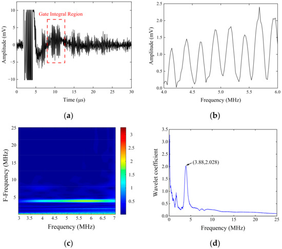
Figure 14.
Detection signal and its signal processing results. (a) Short-period excitation echo signal. (b) EMAR spectrum diagram. (c) Energy density separation distribution diagram. (d) Energy density distribution curve.
Next, we performed 360-degree rotation scanning along the inner edge of the specimen by the locations of the 24 split lines indicated above for each specimen. The frequency interval in the appropriate spectrum signal of each group of test data was extracted using the Δf value, and the results are displayed in Figure 15 as a result of keeping the EMAT coil’s center point on a concentric circle during rotation. The polar coordinate diagram makes it abundantly evident that when the transducer was positioned at a single thickness of the specimen, the frequency interval recorded by EMAR was nearly constant. As shown in Figure 15a, when the rotation angle of the transducer was in the range of 0~75 degrees and 105~360 degrees, the interval Δf fluctuated in a small range around 0.155 MHz, and the corresponding thickness of the specimen could be calculated by Formula (6) to be about 10.09 mm, with an error of 0.9% from the true value. When the rotation angle of the transducer was in the range of 75~105 degrees, the interval Δf fluctuated in a small range around 0.26 MHz, and the corresponding specimen thickness could be calculated by Formula (6) to be about 6.05 mm, with an error of 0.8% from the true value. Meanwhile, for the case with a sector angle of 30 degrees and 45 degrees, because the thickness step surfaces were located inside the same sound field of the transducer at 75 degrees of the specimen, the resonance intervals obtained were consistent. If the rotation scanning angle is set smaller, the sector angle information will be more perfect and precise.
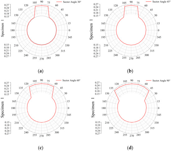
Figure 15.
Calculation results of frequency interval of specimen 1. (a) Sector angle 30°. (b) Sector angle 45°. (c) Sector angle 60°. (d) Sector angle 90°.
In addition, the spectrum analysis chart acquired by frequency sweep should include the information corresponding to the two thicknesses when the transducer is placed at the thickness step surface of the specimen because of the difference in coil excitation signals on both sides of the thickness. However, the calculated result from the actual detection data showed that the frequency interval in the final spectrum signal Δf always tended to the side of the smaller value of thickness, and the value was a jump change process. Currently, the results obtained can only be used to assess one type of thickness information. Therefore, a more accurate scan is required since the analysis of the changing rule of Δf value can only realize the approximate location of the thickness step surface.
In the following experiment, we utilized the moving scanning method outlined in Section 2.2 to determine the thickness step surface of a specimen with a sector angle of 45°. The signal separation process is shown in Figure 16. According to this approach, the frequency spectrum curves of the transducer’s entire 6 mm and 10 mm thickness sides were first collected by frequency scanning, and the corresponding frequency of each curve’s peak point was then retrieved as the reference frequency to separate the data from the mixed thickness spectrum curve detected by the moving coil. After that, we translated the transducer from the side with the large thickness to the side with the small thickness (defined as Move Mode 1). Recording the spectrum data from each scan, each translation step value was 10% of the coil diameter. The schematic diagram of data separation at a 50% moving distance is shown in Figure 16a–c. The peak points of the mixed spectrum were retrieved based on the determined reference frequency, after which processing involving zero padding and linear interpolation was carried out to produce the appropriate separation results and finish the data separation process.
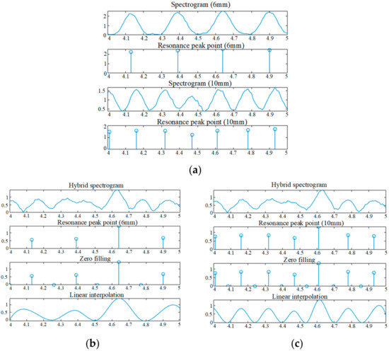
Figure 16.
Diagram of the signal separation process. (a). Mixed spectrum diagram. (b) Separation results of small thickness data. (c) Separation results of large thickness data.
Then, all the test results were processed by the FFEDP algorithm, the maximum energy density value of each group of thickness data was recorded, and the total EDR was calculated by Formula (9); the results are shown in Table 3. The data in the table show that when the moving distance of the coil increased, the maximum energy density values showed monotonic changes, which is consistent with the simulation results. The EDR change curve on both sides of the step surface also clearly intersected at a coil moving distance of 40% to 50%, allowing for a precise determination of the step surface’s position.
Table 3.
EDR result of Move Mode 1.
Similar to the process described above, the transducer was moved and scanned from the specimen’s small thickness side to its large thickness side (defined as Move Mode 2). The calculation results of its EDR are shown in Table 4. This method is accurate because the changing trend is consistent with the findings of the research shown above. By summarizing the results of EDR obtained from all tests, the amplitude quantification result of the specimen can be obtained, as shown in Figure 17. The figure shows that this method is capable of characterizing the specimen’s overall thickness as well as enabling the visual identification of the thickness step surface. Simultaneously, the same approach was employed to test the remaining three specimens with varying sector angles, and it is clear that this procedure had the same capacity for categorization.
Table 4.
EDR result of Move Mode 2.
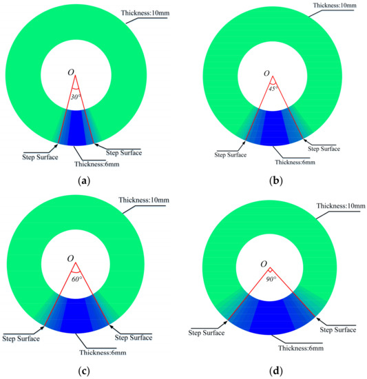
Figure 17.
EDR amplitude quantification diagram of specimen 1. (a) Sector angle 30°. (b) Sector angle 45°. (c) Sector angle 60°. (d) Sector angle 90°.
To validate the applicability of this method, the same method was used to rotate scan the second batch of specimens, with each sector angle at a 15-degree interval, and the results are shown in Figure 18.
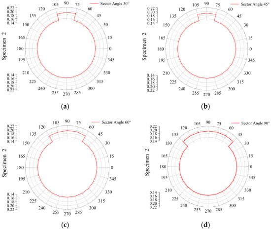
Figure 18.
Calculation results of the frequency interval of specimen 2. (a) Sector angle 30°. (b) Sector angle 45°. (c) Sector angle 60°. (d) Sector angle 90°.
When compared to the result of specimen 1, the Δf estimated by this set of detection data was altered (the value was between the theoretical Δf values corresponding to the two thicknesses), but the bias toward the tiny thickness value was maintained, necessitating the usage of the moving scan technique of detection.
Results for the EDR and the quantitative distribution diagram obtained by translation scanning specimen 2 with the same 45-degree sector angle are shown in Table 5 and Figure 19, respectively. The moving direction (MD) of the transducer was consistent with specimen 1. As the moving distance rose, more of its maximum energy density value conformed to the aforementioned change rule, according to the chart data, and the image created by the amplitude quantization distribution had a remarkable ability to visualize thickness data. Figure 19a–d further demonstrates the use of this process on various sector angle specimens.
Table 5.
EDR results of the transducer at different moving distances.
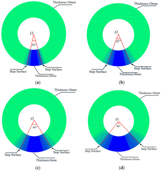
Figure 19.
EDR amplitude quantification diagram of specimen 2. (a) Sector angle 30°. (b) Sector angle 45°. (c) Sector angle 60°. (d) Sector angle 90°.
5. Conclusions
In this paper, a moving scanning method of EMAR was proposed for identifying the thickness step surface of metal specimens. The proposed method utilized the FFEDP algorithm, which can not only achieve accurate extraction of step thickness information, but also achieve effective separation of step thickness information. The finite element simulation models at different positions were built to show the extraction process of different sound field spectrum signals, and the accurate extraction and separation of step thickness information could be achieved by analyzing the sound field source signals on both sides of the step surface separately using the EMAR method. Then, through a moving scan of the step surface, the FFEDP algorithm was used to process and analyze the EDR of the spectrum signal under different moving distances, which verified its feasibility in step surface recognition. Subsequently, the method was verified by experiments. According to the experimental results, with the equidistant movement and scanning of the transducer coil, the ratio between the maximum points of the energy density curve on both sides of the step surface had the opposite change rule. Visual identification and characterization of the thickness interface can be obtained through the study of the ratio change relationship and amplitude quantization processing. The final results of the experiment are in agreement with the simulation results, in which a slight error existed because the finite element simulation ignores the influence of coil area proportion on coil movement, but the changing trend of the EDR is consistent.
Therefore, the method proposed in this paper can well solve the problem of the traditional ultrasonic thickness measurement technology, i.e., it is difficult to extract the arrival time of its signal because of the multimodal acoustic wave mixing in the ultrasonic testing process. The method can serve as a new processing method to address the problem of the frequency spectrum obtained by the specimen, i.e., its thickness step change cannot be further analyzed during the thickness testing.
Author Contributions
Algorithm perfection, Z.L.; experiment preparation, Q.Z.; writing—original manuscript preparation, Y.S.; manuscript review and editing, Z.C. All authors have read and agreed to the published version of the manuscript.
Funding
This work was supported by National Natural Science Foundation of China under Grant 51807065, Natural Science Foundation of Jiangxi under Grant 20224BAB204053, Funding Program of Jiangxi Graduate Innovation Special Fund (YC2021-S450), State Key Laboratory of Reliability and Intelligence of Electrical Equipment No.EERI_KF2021007, Hebei University of Technology, Key Laboratory of Nondestructive Testing No. S2-KF2007, Fuqing Branch of Fujian Normal University, Fujian Province University.
Institutional Review Board Statement
Not applicable.
Informed Consent Statement
Not applicable.
Data Availability Statement
Not applicable.
Conflicts of Interest
The authors declare no conflict of interest.
References
- Kasztankiewicz, A.; Gańczyk-Specjalska, K.; Zygmunt, A.; Cieślak, K.; Zakościelny, B.; Gołofit, T. Application and properties of aluminum in rocket propellants and pyrotechnics. J. Elem. 2018, 23, 321–331. [Google Scholar]
- Schubbe, J.J. Plate Thickness Variation Effects on Crack Growth Rates in 7050-T7451 Alloy Thick Plate. J. Mater. Eng. Perform. 2010, 20, 147–154. [Google Scholar] [CrossRef]
- Mihaljević, M.; Markučič, D.; Runje, B.; Keran, Z. Measurement uncertainty evaluation of ultrasonic wall thickness measurement. Measurement 2019, 137, 179–188. [Google Scholar] [CrossRef]
- Towsyfyan, H.; Biguri, A.; Boardman, R.; Blumensath, T. Successes and challenges in non-destructive testing of aircraft composite structures. Chin. J. Aeronaut. 2019, 33, 771–791. [Google Scholar] [CrossRef]
- Su, Z.; Ye, L.; Lu, Y. Guided Lamb waves for identification of damage in composite structures: A review. J. Sound Vib. 2006, 295, 753–780. [Google Scholar] [CrossRef]
- Dixon, S.; Edwards, C.; Palmer, S. High accuracy non-contact ultrasonic thickness gauging of aluminum sheet using electromagnetic acoustic transducers. Ultrasonics 2001, 39, 445–453. [Google Scholar] [CrossRef]
- Wu, Y.; Han, L.; Gong, H.; Yang, J.; Li, W. Effect of Coil Configuration on Conversion Efficiency of EMAT on 7050 Aluminum Alloy. Energies 2017, 10, 1496. [Google Scholar] [CrossRef]
- Ashigwuike, E.; Ushie, O.; Mackay, R.; Balachandran, W. A study of the transduction mechanisms of electromagnetic acoustic transducers (emats) on pipe steel materials. Sens. Actuators 2015, 229, 154–165. [Google Scholar] [CrossRef]
- Kim, Y.-K.; Park, I.-K. Evaluation of Thickness Reduction in an Aluminum Sheet using SH-EMAT. J. Korean Weld. Join. Soc. 2010, 28, 74–78. [Google Scholar] [CrossRef]
- Parra-Raad, J.; Khalili, P.; Cegla, F. Shear waves with orthogonal polarisations for thickness measurement and crack detection using emats. NDT E Int. 2020, 111, 102212. [Google Scholar] [CrossRef]
- Zhang, J.; Liu, M.; Jia, X.; Gao, R. Numerical Study and Optimal Design of the Butterfly Coil EMAT for Signal Amplitude Enhancement. Sensors 2022, 22, 4985. [Google Scholar] [CrossRef]
- Zhang, X.; Cheng, J.; Qiu, G.; Tu, J.; Song, X.; Cai, C. Shear Horizontal Circumferential Wave EMAT Design for Pipeline Inspection Based on FEM. Int. J. Appl. Electromagn. Mech. 2020, 64, 913–919. [Google Scholar] [CrossRef]
- Kang, L.; Zhang, C.; Dixon, S.; Zhao, H.; Hill, S.; Liu, M. Enhancement of ultrasonic signal using a new design of Rayleigh-wave electromagnetic acoustic transducer. NDT E Int. 2016, 86, 36–43. [Google Scholar] [CrossRef]
- Li, W.; Jiang, C.; Deng, M. Thermal damage assessment of metallic plates using a nonlinear electromagnetic acoustic resonance technique. NDT E Int. 2019, 108, 102172. [Google Scholar] [CrossRef]
- Cho, S.W.; Ji, B.; Cho, S.H. Detection of Microcrack on Thin Plates Using EMAT-Based Resonant Ultrasonic Spectroscopy. J. Korean Soc. Nondestruct. Test. 2019, 39, 1–6. [Google Scholar] [CrossRef]
- WLi, W.; Jiang, C.; Lan, Z.; Deng, M. Thermal Damage Evaluation in Nickel Plate by Nonlinear Electromagnetic Acoustic Resonance Technique. NDT E Int. 2019, 64, 835–842. [Google Scholar]
- Diguet, G.; Miyauchi, H.; Takeda, S.; Uchimoto, T.; Mary, N.; Takagi, T.; Abe, H. EMAR monitoring system applied to the thickness reduction of carbon steel in a corrosive environment. Mater. Corros. 2022, 73, 658–668. [Google Scholar] [CrossRef]
- Yusa, N.; Song, H.; Iwata, D.; Uchimoto, T.; Moroi, M. Probabilistic analysis of electromagnetic acoustic resonance signals for the detection of pipe wall thinning. Nondestruct. Test. Eval. 2019, 36, 1–16. [Google Scholar] [CrossRef]
- Liu, T.; Pei, C.; Cheng, X.; Zhou, H.; Xiao, P.; Chen, Z. Adhesive debonding inspection with a small EMAT in resonant mode. NDT E Int. 2018, 98, 110–116. [Google Scholar] [CrossRef]
- Li, Y.; Cai, Z.; Chen, L. Detection of Sloped Aluminum Plate Based on Electromagnetic Acoustic Resonance. IEEE Trans. Instrum. Meas. 2021, 71, 1–12. [Google Scholar] [CrossRef]
- Huang, S.; Sun, H.; Wang, S.; Qu, K.; Zhao, W.; Peng, L. SSWT and VMD Linked Mode Identification and Time-of-Flight Extraction of Denoised SH Guided Waves. IEEE Sens. J. 2021, 21, 14709–14717. [Google Scholar] [CrossRef]
- Ritec Inc. Operation Manual, Model Snap-0.25-7, Ritec Advanced Measurement System; Ritec Inc.: Warwick, RI, USA, 2002. [Google Scholar]
- Deng, M.; Wang, P.; Lv, X. Experimental observation of cumulative second-harmonic generation of Lamb-wave propagation in an elastic plate. J. Phys. D Appl. Phys. 2005, 38, 344–353. [Google Scholar] [CrossRef]
- Zhang, Y.; Huang, S.L.; Wang, S.; Zhao, W. Time-frequency energy density precipitation method for time-of-flight extraction of narrowband Lamb wave detection signals. Rev. Sci. Instrum. 2016, 87, 054702. [Google Scholar] [CrossRef] [PubMed]


Disclaimer/Publisher’s Note: The statements, opinions and data contained in all publications are solely those of the individual author(s) and contributor(s) and not of MDPI and/or the editor(s). MDPI and/or the editor(s) disclaim responsibility for any injury to people or property resulting from any ideas, methods, instructions or products referred to in the content. |
© 2023 by the authors. Licensee MDPI, Basel, Switzerland. This article is an open access article distributed under the terms and conditions of the Creative Commons Attribution (CC BY) license (https://creativecommons.org/licenses/by/4.0/).