Microstructural Modeling of the Magnetization Process in Ni₂MnGa Alloy Polytwin Crystals

Abstract

In this article, based on the theory of micromagnetism, a microstructural model of the behavior of the Heusler alloy in a magnetic field is constructed. The dynamics of the magnetic process is described by the Landau–Lifshitz–Gilbert equation. Using the Galerkin procedure, variational equations corresponding to the differential relations of the magnetic problem are written out. For numerical simulation, we consider the problem of magnetization of a Ni${}_2$MnGa alloy polytwin crystals, each grain of which is a twinned variant of martensite and has pronounced anisotropic properties. First, we consider the process of magnetization of a single grain, when an external magnetic field is applied at different angles to the anisotropy axes of twinned variants, and then, based on the results obtained, we plot magnetization curves for various (isotropic and texture-oriented) polycrystalline samples. This paper does not consider the process of detwinning, which can occur in such a material during the magnetization at a sufficiently high external field strength.

1. Introduction

The Ni${}_2$MnGa alloy is of great interest due to the fact that the martensitic transformation in it can be controlled using a magnetic field [1,2,3]. If cooling from the austenitic state (high-temperature phase) with a cubic crystal lattice can be achieved without the application of a mechanical load, then, as a result of realization of direct first-order phase transition, in the martensite phase (tetragonal low-temperature phase) twin structures (twins) are formed. These structures can be detwinned when a stress and/or an external magnetic field is applied, which causes substantial deformation up to 6–10%. At temperatures below the Curie point (in the martensitic state), such materials, being ferromagnets, exhibit spontaneous magnetization even in the absence of an external magnetic field. In each variant of martensite, there is an easy magnetization axis, which is an energetically favorable direction for the spontaneous magnetization vector. Regions composed of interconnected variants of martensite, in which the magnetization vectors have the same direction, form magnetic domains. As a result, in the martensitic state, many magnetic domains are formed with different directions of the magnetization vectors, and it is energetically advantageous for these domains to be coordinated with each other so that such an alloy is not integrally magnetized if no magnetic field is applied. With the action of the latter, the movement of the walls of the magnetic domains, the rotation of the magnetization vectors and the reorientation of martensite variants (detwinning) begin.

Since the processes described above take place at the level of the material structure, the use of micromechanical models [4,5,6,7], in contrast to the phenomenological [8,9,10], makes it possible to obtain constitutive relations without additional assumptions. There are two ways to describe the evolution of the magnetization vector in terms of micromagnetism [11]. The first one is based on minimizing the magnetic energy density functional with certain restrictions on some parameters, for which it is necessary to solve the Euler–Ostrogradsky equation corresponding to the minimum of this functional, or directly minimize the functional, for example, by the finite element method. The second approach uses the Landau–Lifshitz–Gilbert equation in which a strength vector of effective field is a result of application of the Euler–Ostrogradsky operator to the total magnetic energy density functional. In [12], the magnetic energy functional is minimized to describe the evolution of magnetization. For a Ni${}_2$MnGa single crystal, the movement and interaction of the Néel domain walls under the application of a magnetic field are numerically simulated. In [13] the Landau–Lifshitz–Hilbert equation was used for a more complex structure (twinned variant of martensite). In that publication, using the standard Galerkin procedure, variational equations are put in correspondence with the Landau–Lifshitz–Hilbert differential equation and differential equation for the scalar quantity by which the demagnetization vector is determined. This makes it possible to reduce (weaken) the requirements for the smoothness of the solution compared to the original differential equations, and therefore this formulation of the problem is called weak. In [14], the possibilities of each of these two approaches (minimization of the magnetic energy functional and solution to the Landau–Lifshitz–Gilbert equation) to describe the magnetic processes are analyzed and a conclusion about the advantage of using the Landau–Lifshitz–Gilbert equation is made.

Polycrystalline samples, in contrast to single crystals, are easier to manufacture. This gives more opportunities for their use; for example, polycrystalline films can be used in spintronics, actuator and sensor applications. In this case, polycrystalline samples can be not only isotropic, but also textured. A number of works are devoted to the investigation of the structure and properties of such polycrystalline samples. In works [15,16,17,18,19], the single-twinned crystals of Ni-Mn-Ga alloys and a polycrystal created from these elements are studied and magnetization curves for these structures are constructed.

In the present paper, we, using the Landau–Lifshitz–Gilbert equation in the variational form, numerically simulate the process of magnetization of polytwinned crystals of Ni${}_2$MnGa, each grain of which is a twin variant of martensite. Because polycrystalline samples can be isotropic (martensitic twins are randomly oriented) or texture-oriented (there is a predominant direction of martensitic structures orientation), magnetization curves were numerically obtained for various polycrystalline samples.

In this work, the new findings are: (a) the use of variational equations corresponding to the differential formulation for the problem of the magnetization of a ferromagnetic material in a magnetic field, (b) the results obtained within the framework of this approach describing the behavior of a single-twin crystal of Ni-Mn-Ga alloys, and (c) magnetization curves constructed for the polytwinned crystals, each grain of which is a twin variant of martensite.

2. Basic Relations of Micromagnetism

Based on the theory of micromagnetism [11], the magnetization of each crystal cell at a temperature significantly below the Curie temperature is described by the spontaneous magnetization vector $\mathbf{M}$. According to this theory, the length of the magnetization vector is constant: $\left|\mathbf{M}\right|=M_s$, where $M_s$ is the saturation magnetization. This vector in anisotropic materials is directed along the easy magnetization axis A unit vector $\mathbf{m}=\mathbf{M}/M_s$ is set, the dynamics of which is described by the Landau–Lifshitz–Gilbert equation:

$$\frac{\partial \mathbf{m}}{\partial t}=-\gamma (\mathbf{m}\times {\mathbf{H}}_{eff})+\alpha \left(\mathbf{m}\times \frac{\partial \mathbf{m}}{\partial t}\right),$$

(1)

where $\gamma$ is a gyromagnetic ratio, $\alpha$ is a damping (dissipation) parameter, ${\mathbf{H}}_{eff}$ is a strength vector of effective field (see, for example, [13]):

$${\mathbf{H}}_{eff}={\mathbf{H}}_0-\nabla \phi +\frac{2A_{exch}}{{\mu }_0{M}_s}\Delta \mathbf{m}+\frac{2K_{anis}}{{\mu }_0{M}_s}(\mathbf{m}·{\mathbf{p}}_i){\mathbf{p}}_i.$$

(2)

Here, ${\mathbf{H}}_0$ is a strength vector of an applied external field, which in our case does not depend on coordinates (it is constant in space in magnitude and direction), $\phi$ is a scalar magnetic potential that produces the strength vector of internal demagnetization field caused by an applied external field ${\mathbf{H}}_0$ (thus, the magnetic field strength is given by the relation $\mathbf{H}={\mathbf{H}}_0-\nabla \phi$), and the last two terms are the exchange field strength vector ${\mathbf{H}}_{exch}$ and the anisotropy field strength vector ${\mathbf{H}}_{anis}$ which are produced by the volume and surface magnetic charges. In the last two terms ${\mu }_0$ is the permeability of the vacuum, $A_{exch}$ and $K_{anis}$ are the exchange parameter and the anisotropy constant, ${\mathbf{p}}_i$ is the unit vector of the easy axis direction of the variant i. Here, the strength of the magnetoelastic field, which causes magnetostrictive deformation, is not taken into account, since this deformation is very small compared to the phase one and is usually neglected [6].

The scalar magnetic potential $\phi$ is found (see, for example, [12] or [13]) from the solution of the Poisson equation in the region ${\Omega }^{\left(in\right)}$ occupied by the body

$$\nabla ·\nabla \phi =M_s\nabla ·\mathbf{m}\forall \mathbf{x}\in {\Omega }^{\left(in\right)}$$

(3)

and the Laplace equation in the region ${\Omega }^{\left(ex\right)}$ occupied by the surrounding medium

$$\nabla ·\nabla \phi =0\forall \mathbf{x}\in {\Omega }^{\left(ex\right)}.$$

(4)

The natural requirement that $\phi$ must obey is $\phi \to 0$ when $\mathbf{x}\to \infty$. On the $\Gamma$ surface separating the body from its environment, ${\phi }^{\left(in\right)}{{|}_{\Gamma }={\phi }^{\left(ex\right)}|}_{\Gamma }$, where the superscript $\left(in\right)$ refers to the body and the superscript $\left(ex\right)$ to its environment.

The following boundary conditions for $\phi$ must also be satisfied:

$$\begin{array}{c}(\nabla {\phi }^{\left(in\right)}-\nabla {\phi }^{\left(ex\right)}){|}_{\Gamma }·\mathbf{n}=M_s\mathbf{m}·\mathbf{n},\\ (\nabla {\phi }^{\left(in\right)}-\nabla {\phi }^{\left(ex\right)}){|}_{\Gamma }·\mathbf{\tau }=0,\end{array}$$

(5)

where $\mathbf{\tau }$ is unit tangent and $\mathbf{n}$ is the unit outer normal.

The magnetization vector must satisfy the boundary condition (see, for example, [13]):

$$2A_{exch}\left[\mathbf{m}\times (\mathbf{n}·\nabla \mathbf{m})\right]{|}_{\Gamma }=\mathbf{0}.$$

(6)

From the relation $\mathbf{m}·\mathbf{m}=1$ we obtain for the normal derivative $\mathbf{n}·\nabla (\mathbf{m}·\mathbf{m})=0$, that leads to $(\mathbf{n}·\nabla \mathbf{m})·\mathbf{m}=0$, that is, the vector $(\mathbf{n}·\nabla \mathbf{m})$ is perpendicular to the vector $\mathbf{m}$. Then the equality (6) will be satisfied only if at least one of the multipliers is zero. As $\mathbf{m}\ne \mathbf{0}$, another vector must be equal to zero, and this is the Neumann boundary condition for the vector $\mathbf{m}$:

$$(\mathbf{n}·\nabla \mathbf{m}){|}_{\Gamma }=\mathbf{0}.$$

To describe the distribution of the magnetization vector in the body, it is necessary to solve the differential Equations (1), (3) and (4) with boundary conditions (5) and (6). The strength vector of effective field ${\mathbf{H}}_{eff}$ in Equation (1) is determined by the relation (2). The relations (3) and (4) require, at least, the existence of a second derivative with respect to the coordinates for the function $\phi$, and the relation (2) for the function $\mathbf{m}$. Using the Galerkin procedure, we realize the so-called weak (variational) formulation of the problem and reduce the requirements for the smoothness of these functions. The constructed variational equations are given in the work [13] and have the following form:

$${\int }_{{\Omega }^{\left(in\right)}}(\nabla \phi -M_s\mathbf{m})·\nabla \delta \phi d{\Omega }^{\left(in\right)}+{\int }_{{\Omega }^{\left(ex\right)}}\nabla \phi ·\nabla \delta \phi d{\Omega }^{\left(ex\right)}=0$$

(7)

and

$$\begin{array}{c}{\int }_{{\Omega }^{\left(in\right)}}({\mathbf{m}}_{*}\times \mathbf{v}+\alpha \mathbf{v}+\lambda {\mathbf{m}}_{*})·\delta \mathbf{v}d{\Omega }^{\left(in\right)}-\hfill \\ -\gamma {\int }_{{\Omega }^{\left(in\right)}}\left({\mathbf{H}}_0-\nabla \phi +\frac{2K_{anis}}{{\mu }_0{M}_s}[({\mathbf{m}}_{*}+\theta \tau \mathbf{v})·{\mathbf{p}}_i]{\mathbf{p}}_i\right)·\delta \mathbf{v}d{\Omega }^{\left(in\right)}+\\ \hfill +\frac{2\gamma A_{exch}}{{\mu }_0{M}_s}{\int }_{{\Omega }^{\left(in\right)}}[{(\nabla \mathbf{m})}_{*}^T+\theta \tau {(\nabla \mathbf{v})}^T]··\nabla \delta \mathbf{v}d{\Omega }^{\left(in\right)}+{\int }_{{\Omega }^{\left(in\right)}}({\mathbf{m}}_{*}·\mathbf{v})\delta \lambda d{\Omega }^{\left(in\right)}=0.\end{array}$$

(8)

The $\theta$-scheme was used to write relation (8): $\mathbf{m}\left(t\right)$ at the current time t is represented as ${\mathbf{m}}_{*}+\theta \tau \mathbf{v}$, where ${\mathbf{m}}_{*}=\mathbf{m}\left(t_{*}\right)$ is the magnetization at the previous time $t_{*}$, $\tau =t-t_{*}$ is the time step, $\theta \in [0,1]$, $\mathbf{v}=\partial \mathbf{m}/\partial t$, $\lambda$ is the Lagrange multiplier to meet the conditions ${\mathbf{m}}_{*}·\mathbf{v}=0$ and ${\mathbf{m}}_{*}·\delta \mathbf{v}=0$ and the superscript T means the operation of transposing for the second rank tensor.

To find $\phi$, $\mathbf{v}$ and $\lambda$, it is necessary to solve coupled variational Equations (7) and (8). Numerical realization of these equations are implemented by the finite element method. The external magnetic field is applied in accordance with the step-by-step procedure (external problem). Within each such step, in accordance with the $\theta$-scheme mentioned above, another, internal $\tau$ time step is carried out, which makes it possible to describe the evolution of the magnetization vector $\mathbf{m}$ at a given (applied and fixed) external magnetic field. At each such step, the constructed connected variational Equations (7) and (8) are solved and allow us to determine $\phi$, $\mathbf{v}$ and $\lambda$ (internal problem). Knowing the vector $\mathbf{v}$, we define the vector $\mathbf{m}={\mathbf{m}}_{*}+\tau \mathbf{v}$, which will be the initial for the next internal time step. In order to reduce the computational error, the vector $\mathbf{m}$ is corrected so that its length remains unit:

$$\mathbf{m}=\frac{{\mathbf{m}}_{*}+\tau \mathbf{v}}{|{\mathbf{m}}_{*}+\tau \mathbf{v}|}.$$

The solution of the internal problem continues until the values of $\mathbf{v}$ at the current and previous steps are almost the same (satisfy the condition of exiting this process). In our case, it required 3000 internal time steps. After that, we move on to the next time step for the external problem.

At the first stage, in the absence of an external magnetic field, the initial magnetization distribution $\mathbf{m}$ is set and, solving variational equations, the initial boundaries of the magnetic domains and distribution of the magnetization vectors in them are determined. The resulting magnetic structure is the initial one for the subsequent application of an external magnetic field.

The stability of the numerical solution is provided by the choice of the parameter $\theta$: if $\theta >0.5$, the scheme will be stable for any steps in time and space.

3. Statement of the Problem

For numerical simulation, we consider the problem of magnetization of a Ni${}_2$MnGa alloy polytwin crystals, each grain of which is a twinned variant of martensite and has pronounced anisotropic properties. First, we consider the process of magnetization of a single grain, when an external magnetic field is applied at different angles to the anisotropy axes of twinned variants, and then, based on the results obtained, we plot magnetization curves for various polycrystalline samples. This paper does not consider the process of detwinning, which can occur in such a material during the magnetization at a sufficiently high external field strength. This process is supposed to be taken into account in the future.

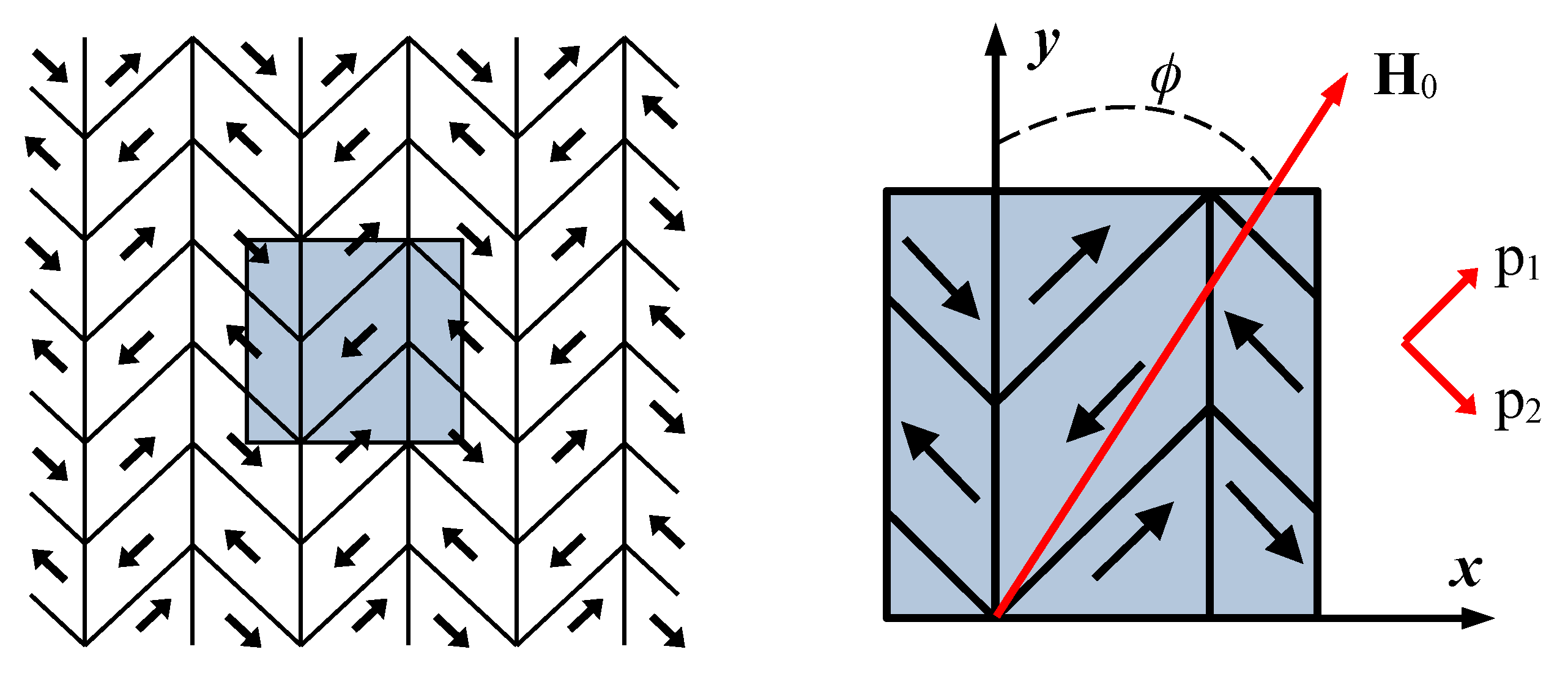
Figure 1 shows the structure of the twinned variant of martensite (the arrows show the magnetization vectors directed along or against the short axes in each variant of martensite—the anisotropy axes ${\mathbf{p}}_1$ for the variant 1 and ${\mathbf{p}}_2$ for the variant 2, directed at angles ${45}^{\circ }$ and $-{135}^{\circ }$ to the axes x and y for the variant 1 and $-{45}^{\circ }$ and ${135}^{\circ }$ to the axes x and y for the variant 2). With this distribution, the sample is integrally non-magnetized unless a magnetic field is applied. Let us determine the size of the computational domain (blue square in Figure 1) 380 nm × 380 nm, taking into account the fact that martensitic plates in the Ni${}_2$MnGa alloy have a characteristic size of about 100–200 nm. To set periodic conditions, the region under consideration is duplicated along the x and y axes. As a result, we obtain the evolution of the magnetization distribution in the sample with an increase in the external magnetic field, as well as magnetization curves for each direction (dependences of the average value of the magnetization projection on the axis along which the external magnetic field is directed on the applied field). Consider the application of an external magnetic field ${\mathbf{H}}_0$ to such a sample in the $(x,y)$ plane at different angles to the y axis—from $0^{\circ }$ to ${90}^{\circ }$ (17 directions in total, which are specified by the angle $\varphi$).

For Ni${}_2$MnGa, we set the following parameters: $M_s=6.015·{10}^5$ A/m is the saturation magnetization, $K_{anis}=2.5·{10}^5$ J/m ${}^3$ is the magnetocrystalline anisotropy constant [6,20], $A_{exch}=2·{10}^{-11}$ J/m is the exchange constant [6,7]. The order of the domain wall thickness for such material is $\Delta \approx \sqrt{A_{exch}/K_{anis}}\approx 9$ nm ([11]). For numerical calculation, we have made all the relations dimensionless by introducing the characteristic size $l_0=3.8\mathrm{nm}$ and energy ${\psi }_0={\mu }_0$$M_s^2=4.55·{10}^5$ J/m${}^3$. The characteristic size was chosen from the condition to the domain wall that had approximately two characteristic sizes. As a result, we obtain the following dimensionless parameters:

$${\tilde{M}}_s=1;{\tilde{K}}_{anis}=\frac{K_{anis}}{{\psi }_0}\approx 0.54;{\tilde{A}}_{exch}=\frac{A_{exch}}{{\psi }_0{l}_0^2}\approx 3.$$

We also make dimensionless the external magnetic field ${\tilde{\mathbf{H}}}_0={\mathbf{H}}_0/M_s$ and introduce the notation ${\tilde{H}}_0=\left|{\tilde{\mathbf{H}}}_0\right|$.

When solving the variational Equation (8), it is assumed that the gyromagnetic ratio $\gamma =2.21·{10}^5$ m/(A·s) and the damping (dissipation) parameter $\alpha =0.5$. The time step was set as $\tau =\gamma M_{s}t=0.05$, $\theta =0.6$. This problem was solved by the finite element method (FEM) using open-source computing platform FEniCS (https://fenicsproject.org accessed on 24 June 2022).

A regular grid consisting of 5184 finite elements was set. The blue square in Figure 1 was divided into 1296 equal squares, each of the resulting squares was divided diagonally into four equal triangles. The periodicity conditions of the solution are imposed. A quadratic approximation was set for the vector $\mathbf{v}$, and linear for $\phi$ and $\lambda$. ${\tilde{H}}_0$ increased from 0 to $1.5$ with increments of ${\tilde{h}}_0=0.01$. Within each step of the applied external magnetic field, 3000 time steps were realized to fulfill the convergence condition of the solution.

4. Results of Numerical Simulation

We construct the average value of the magnetization projection on the axis along which the external magnetic field is directed:

$$\tilde{m}=<m_{\left|\right|}>\frac{1}{S}{\int }_{{\Omega }^{\left(in\right)}}\left(\mathbf{m}·\frac{{\tilde{\mathbf{H}}}_0}{{\tilde{H}}_0}\right)d{\Omega }^{\left(in\right)},$$

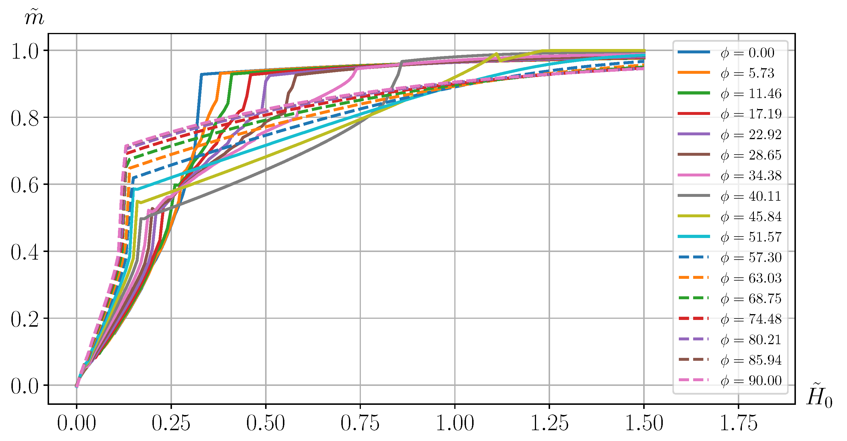
where S is the area of the considered domain. Figure 2 shows the dependences of $\tilde{m}$ on the modulus ${\tilde{H}}_0$ for different directions (angles $\varphi$) of an external magnetic field application. The obtained magnetization curves show strongly anisotropic magnetic properties in the twinned martensite of the Ni${}_2$MnGa alloy.

It can be seen from Figure 2 that there is a significant difference in the magnetization of the twinned variant of martensite for angles $\varphi$ from $0^{\circ }$ to ${45}^{\circ }$ and from ${45}^{\circ }$ to ${90}^{\circ }$. At the initial stage, the application of a magnetic field in a direction close to the x axis leads to a stronger magnetization than the application of a magnetic fields in a direction close to the y axis. However, with an increase in the external magnetic field, the growth of magnetization accelerates for angles $\varphi$ from $0^{\circ }$ to ${45}^{\circ }$ and slows down for angles $\varphi$ from ${45}^{\circ }$ to ${90}^{\circ }$.

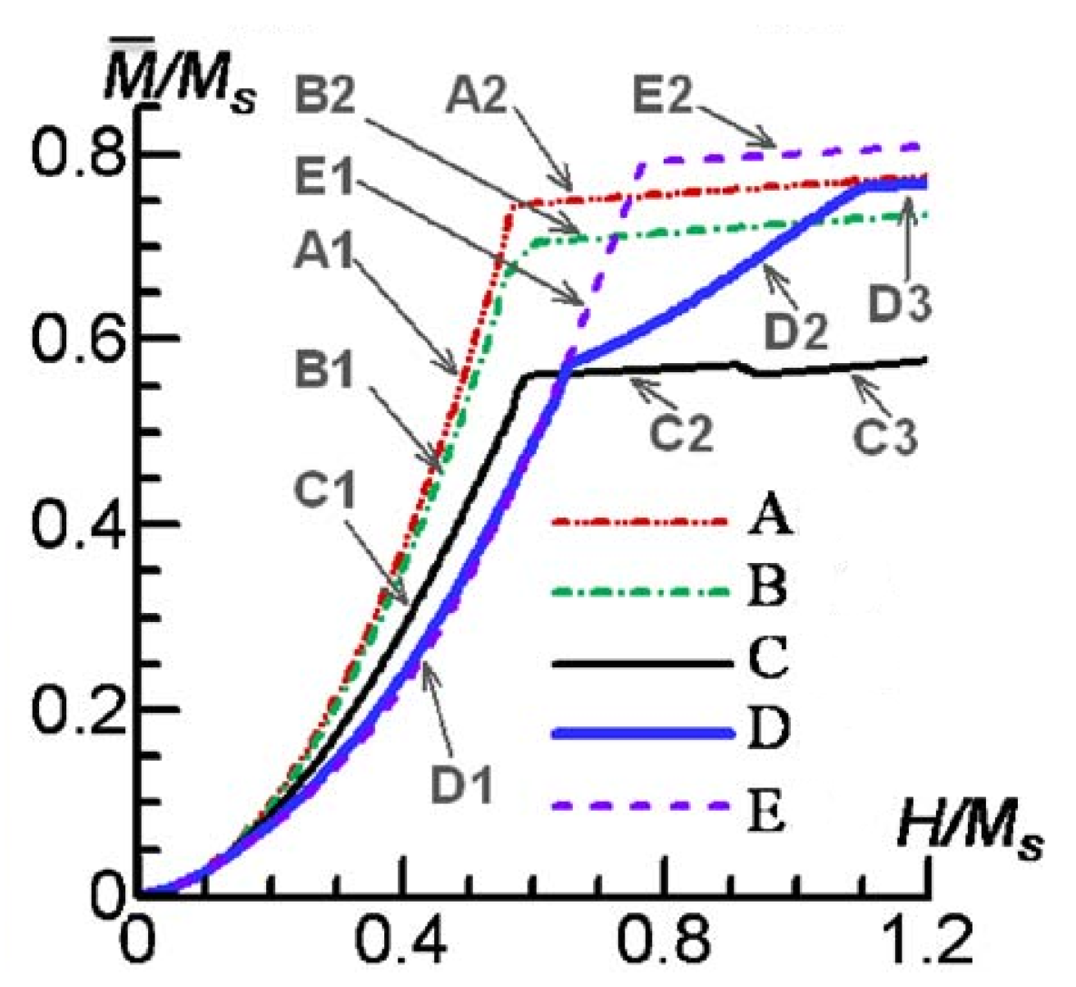
The results obtained can be qualitatively compared with the results presented in [21] for twinned FePt crystals since we do not have similar results for the Ni${}_2$MnGa alloy (see Figure 3). In this paper, the magnetization curves obtained by applying an external magnetic field at different angles show a similar behavior: the mechanism of motion of the walls of magnetic domains is realized faster when a magnetic field is applied along the x axis; however, after the disappearance of unfavorably oriented magnetic domains, the material magnetization is higher when the field is applied along the y axis. Moreover, the magnetization curve when a magnetic field is applied at an angle of ${70}^{\circ }$ to the y axis (comparable with the curve at $\varphi =68.{75}^{\circ }$ in our case) practically coincides with the curve obtained when the field is applied along the x axis; two kinks are observed on the magnetization curve when a magnetic field is applied at an angle of ${20}^{\circ }$ to the y axis (comparable with the curve at $\varphi =17.{19}^{\circ }$ in our case).

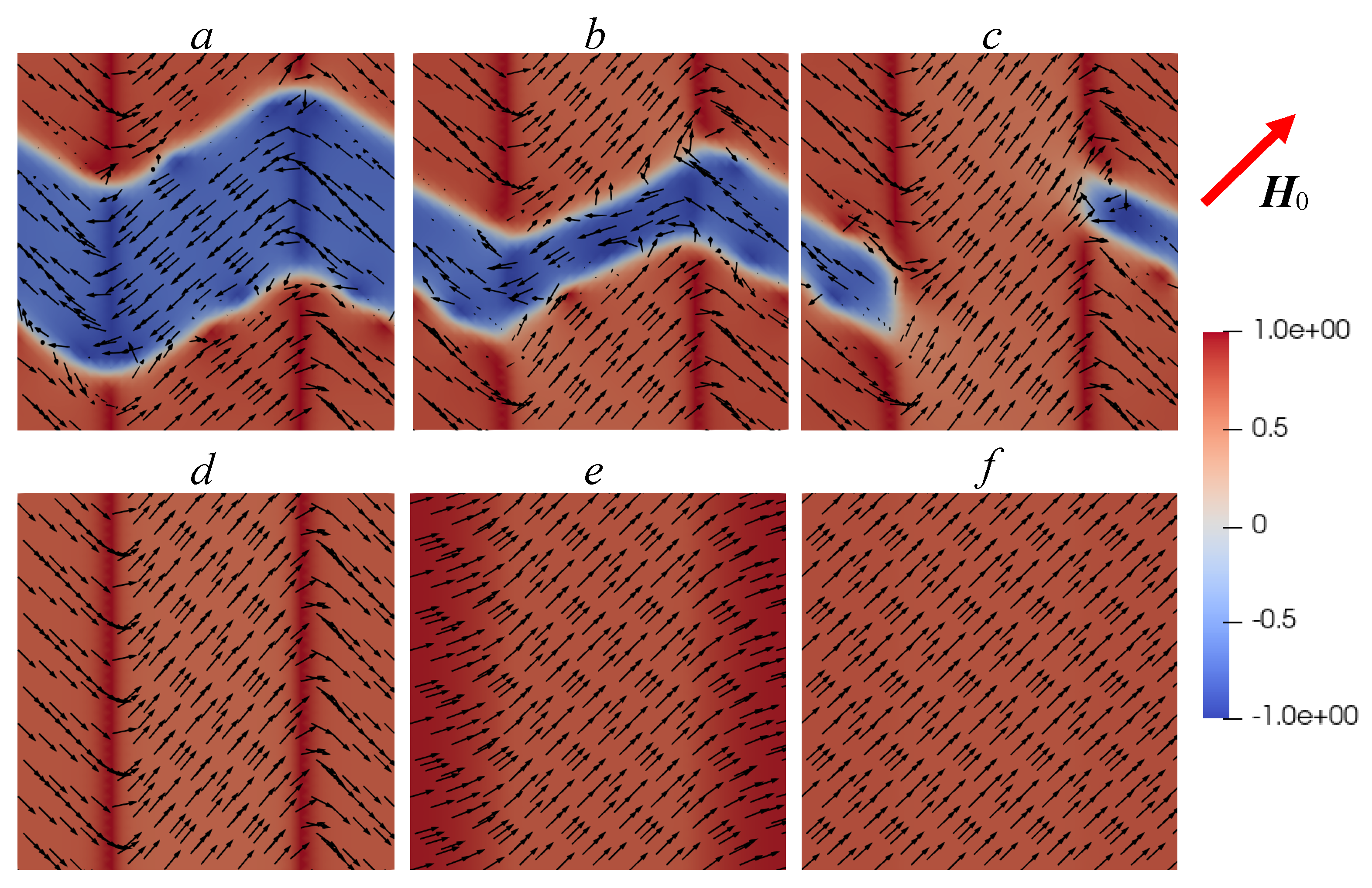
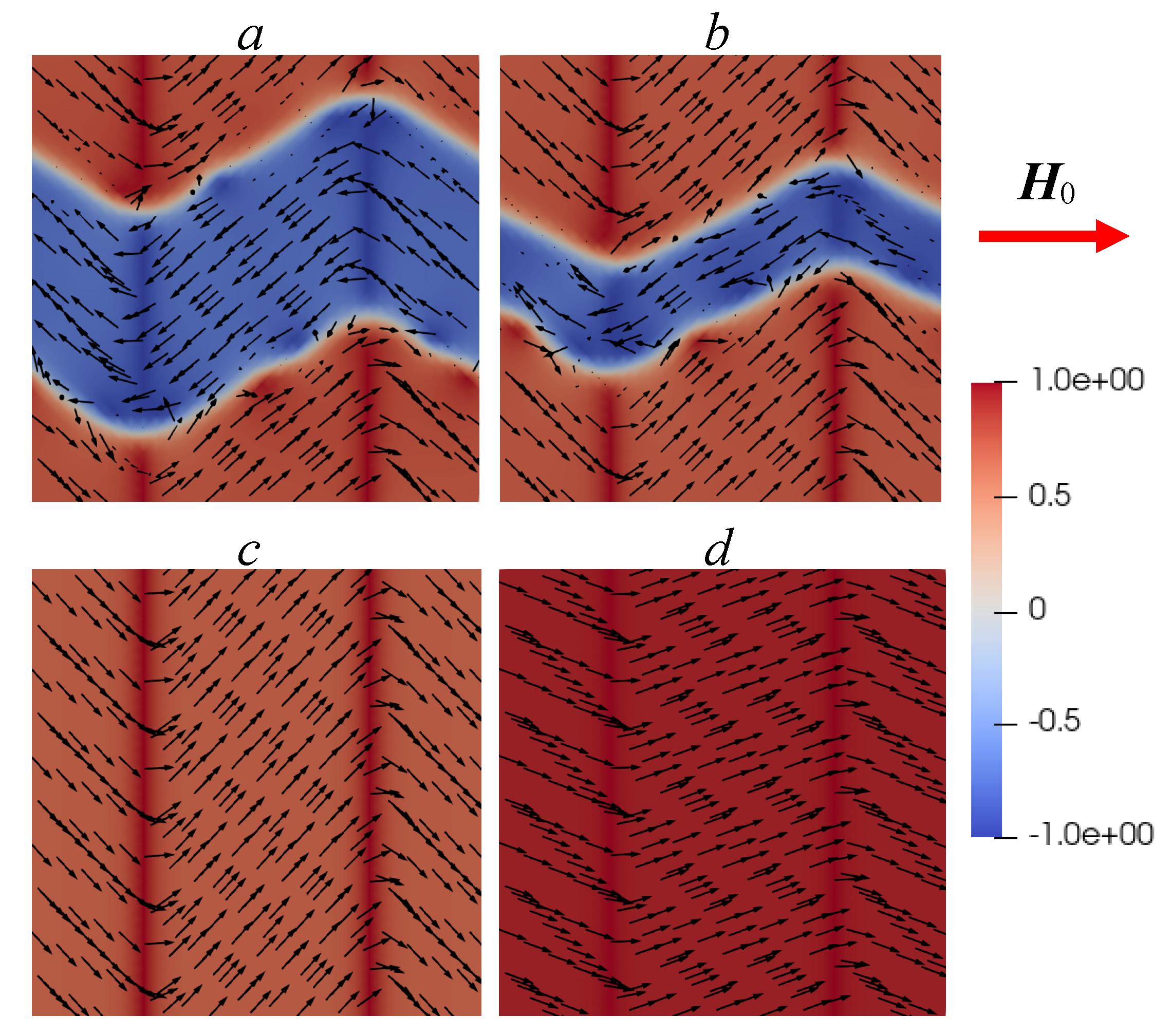
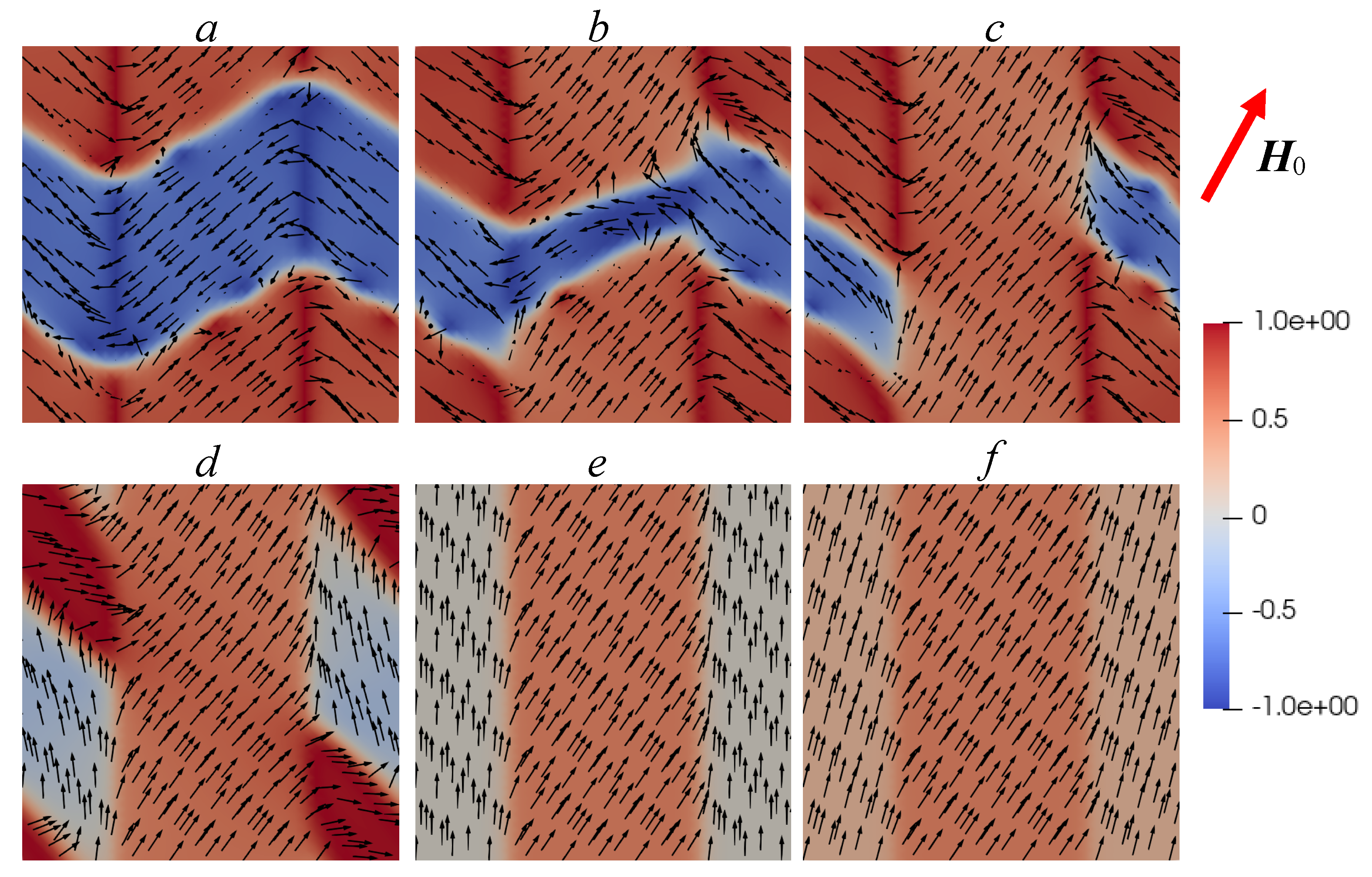
This difference in the magnetization curves can be explained by the fact that the process of evolution of the magnetic structure depends on the direction of the external magnetic field with respect to the anisotropy axes of the twinned variant of martensite. Figure 4, Figure 5, Figure 6 and Figure 7 show four cases of the evolution of the magnetization vector in an external magnetic field, depending on the angles at which this field is applied to the y axes. The arrows in these figures show the projections of the vector $\mathbf{m}$ onto the plane $(x,y)$ for different values of the external magnetic field ${\tilde{H}}_0$ applied at angles $\varphi =0^{\circ }$ (Figure 4), $\varphi =28.{65}^{\circ }$ (Figure 5), $\varphi =45.{84}^{\circ }$ (Figure 6) and $\varphi ={90}^{\circ }$ (Figure 7) to the y axis. The color of the $m_x$ component is displayed in such a way that the areas where $m_x=1$ are red, and the areas where $m_x=-1$ are blue. Areas with other values of $m_x$ are shown in the gradation of these colors according to the scales shown in these figures on the right. It can be seen that at the initial stage, magnetization occurs due to the motion of the walls of the magnetic domains, and then due to the rotation of the magnetization vectors. A change in the main mechanism of magnetization leads to the appearance of kinks in the magnetization curves (see Figure 2) and occurs at different values of ${\tilde{H}}_0$ depending on the direction of the external magnetic field application.

A single crystal was considered above, to which an external magnetic field was applied at different angles in the $xy$ plane. Now, fixing the direction of the external field and placing the same calculated region shown in Figure 1 at different angles to it, we, using the curves shown in Figure 2, describe the magnetization of this representative composite region, which models a polycrystal with a different arrangement of twins in the plane. With this approach, the magnetic interaction of these regions is not considered and the question of it remains open. In order to specify the location of single crystals in a polycrystal, we introduce, in addition to the coordinate system $(x,y)$ associated with the polycrystal, the coordinate systems $(x_j,y_j)$ associated with single crystals (see Figure 8). The location of the crystal j in the polycrystal is determined by the angle ${\varphi }_j$ between the axis $y_j$ and x.

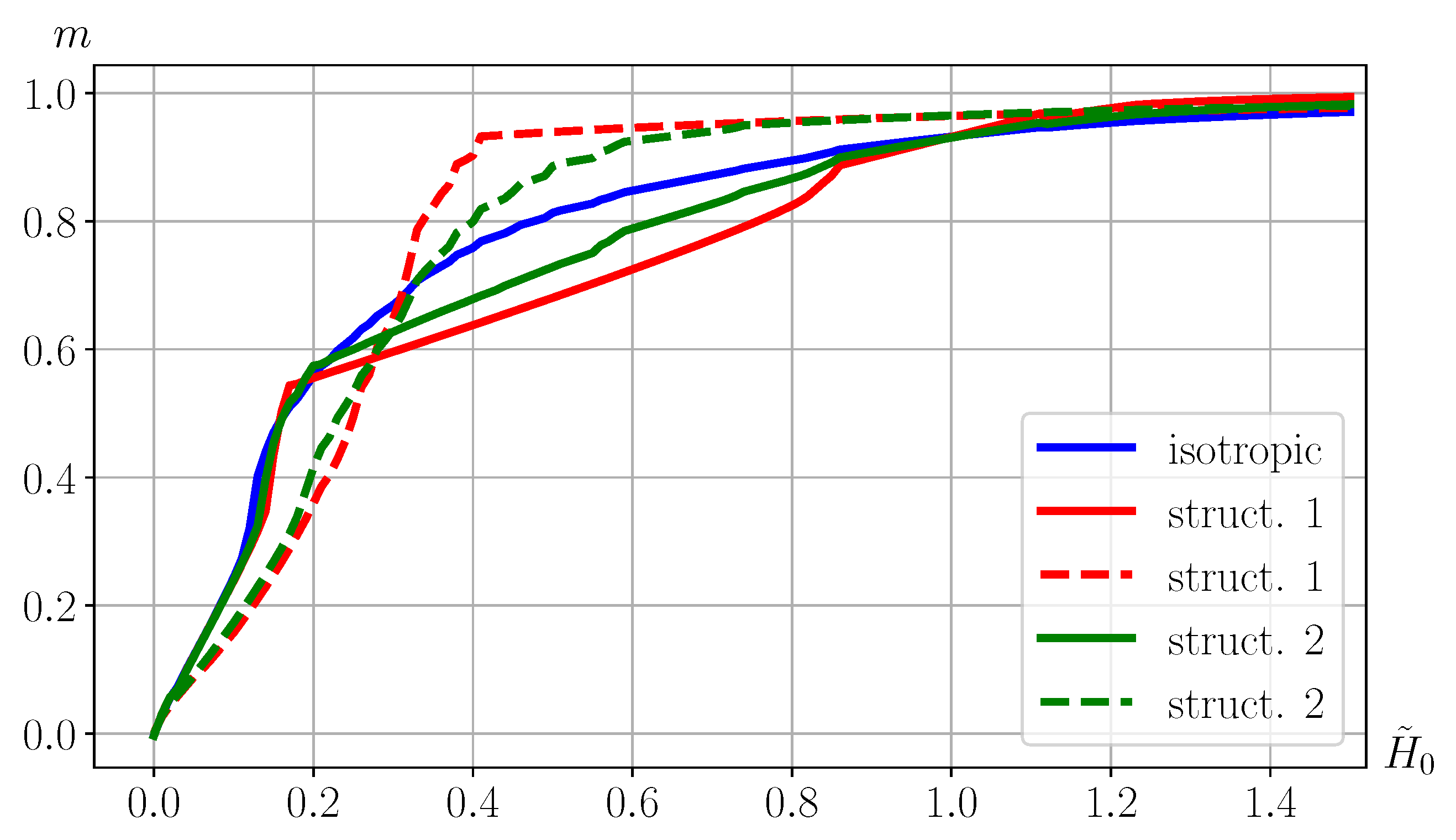
We consider three types of polycrystalline samples:

(1)

isotropic polycrystal—martensitic twins are randomly oriented (17 twinned crystals are located at angles ${\varphi }_j=0^{\circ },\dots ,{90}^{\circ }$ according to Figure 2 and occupy equal areas);

(2)

texture-oriented polycrystal—there is a predominant direction of martensitic structures orientation (3 twinned crystals are located at angles ${\varphi }_j=40.{11}^{\circ },45.{84}^{\circ },51.{57}^{\circ }$ according to Figure 2 and occupy equal areas)—structure 1;

(3)

texture-oriented polycrystal—there is a predominant direction of martensitic structures orientation (5 twinned crystals are located at angles ${\varphi }_j=34.{38}^{\circ },40.{11}^{\circ },45.{84}^{\circ },51.{57}^{\circ },57.{30}^{\circ }$ and occupy equal areas)—structure 2.

The solid lines in Figure 9 show the curves for such polycrystals when an external magnetic field is applied along the x axis. The difference is observed in a magnetic field from ${\tilde{H}}_0=0.2$ to ${\tilde{H}}_0=1$, when the main magnetization mechanism is the rotation of the magnetization vectors towards the applied magnetic field. The dashed lines show the magnetization curves for textured polycrystals when a magnetic field is applied at an angle of ${45}^{\circ }$ to the x and y axes (for an isotropic polycrystal, the magnetization curve in this case completely coincided with the curve corresponding to the field acting along the x axis). For texture-oriented polycrystals, the magnetization curves differ depending on the direction of the applied magnetic field, since such polycrystals are anisotropic.

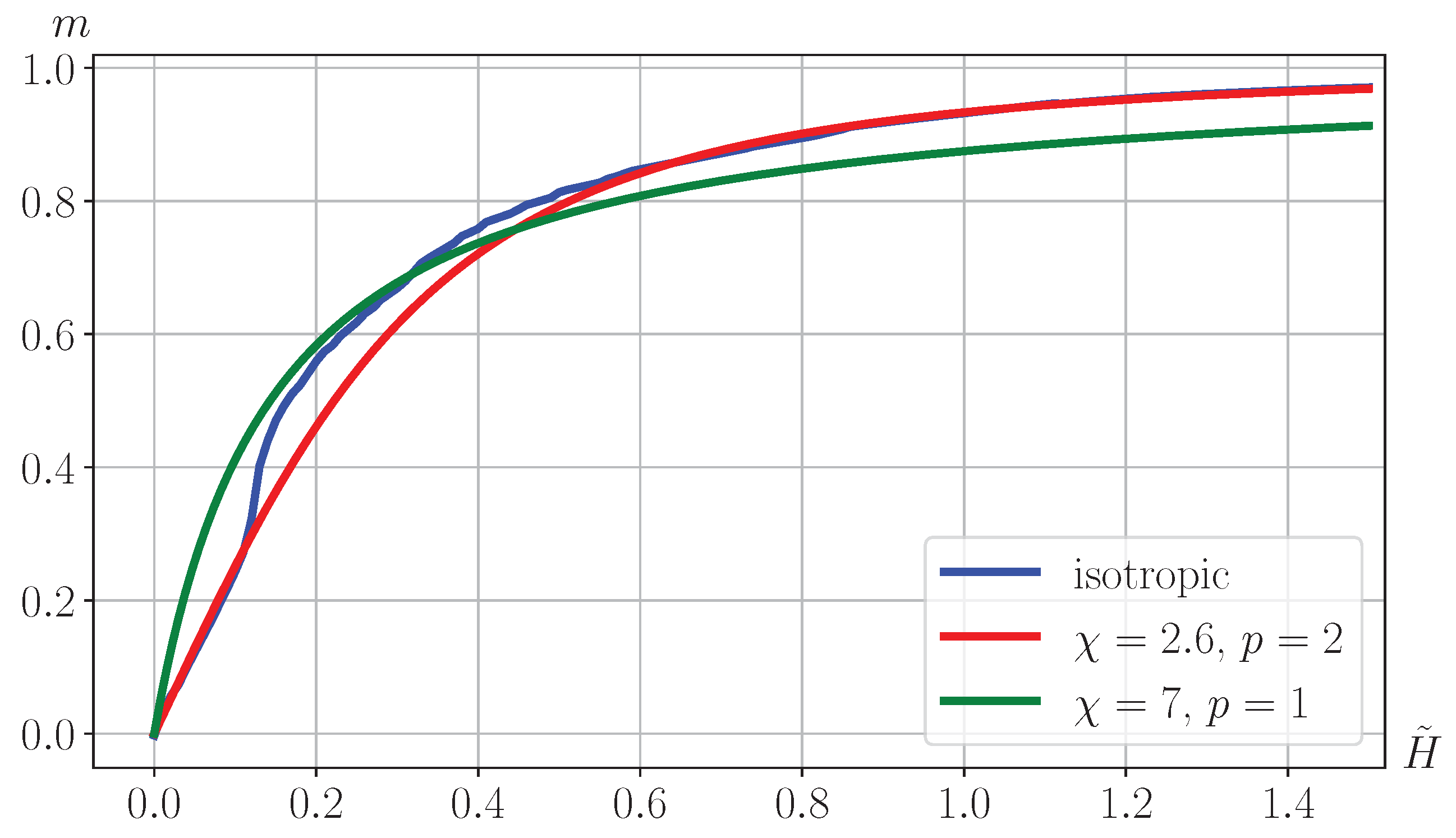
To approximate the obtained magnetization curve of an isotropic polycrystal, we generalize the Fröhlich–Kenelly formula (see, for example, [22]) by adding a constant p as follows:

$$\mathbf{M}={\displaystyle \frac{\chi }{{\left(1+{\left({\displaystyle \frac{\chi H}{M_s}}\right)}^p\right)}^{1/p}}}\mathbf{H},$$

(9)

which coincides with the Fröhlich–Kenelly formula for p = 1. Here $\chi$ is the initial susceptibility and p is a parameter that sets the rate of exit from the linear section to the saturation section. Figure 10 shows the magnetization curves obtained numerically for a polycrystal (blue curve in Figure 9) and by Formula (9) (red and green curves), where $\tilde{\mathbf{H}}=\mathbf{H}/M_s$ and $\tilde{H}=\left|\tilde{\mathbf{H}}\right|$. It can be seen that at $p=2$ and $\chi =2.6$ (red curve) there is good agreement with the magnetization curve obtained numerically in the initial section and when reaching saturation.

5. Conclusions

In the article, the problem of magnetization of a single-twinned variant of martensite and polytwin crystals of a Ni${}_2$MnGa alloy is solved numerically by the finite element method within the framework of the theory of micromagnetism. The dynamics of the magnetic process is described by the Landau–Lifshitz–Gilbert equation to which, like other differential equations and boundary conditions of the theory of magnetism, variational equations are put in accordance. This made it possible to significantly reduce the requirements for the smoothness of the problem solution. Magnetization curves are obtained for applying an external magnetic field at different angles to the anisotropy axes of twinned variants. A change in the main mechanism of magnetization leads to the appearance of kinks in the magnetization curves and occurs at different values of the external magnetic field depending on the direction of this field. Moreover, the magnetization curves were obtained for various types of polycrystals (isotropic and texture-oriented). For textured polycrystals, the magnetization curves differ depending on the direction of the applied magnetic field, since such polycrystals are anisotropic.