Magnetohydrodynamic Effects on Third-Grade Fluid Flow and Heat Transfer with Darcy–Forchheimer Law over an Inclined Exponentially Stretching Sheet Embedded in a Porous Medium

Abstract

The major aim of the current investigations is to study the magnetohydrodynamic effects on heat and mass transfer phenomena in third-grade fluid past an inclined exponentially stretching sheet fixed in a porous medium with Darcy–Forchheimer law influence. The constitutive equations compatible for heat and mass transportation in third-grade fluid in terms of partial differential equations are modeled. These partial differential equations are then converted to ordinary differential equations by using suitable similarity variables formulation. The transformed flow model is solved by using MATLAB built-in numerical solver bvp4c. Effects of pertinent parameters on physical properties that are velocity field, temperature field and mass concentration along with skin friction coefficient, Nusselt number and Sherwood number are demonstrated in graphs and tables. The impact of dimensionless numbers on the physical properties is analyzed and discussed with a physical view point at angle $\alpha =\pi /6$ (inclined sheet). It is seen that as the third-grade fluid parameter $\left(0.1\le \beta \le 11\right)$ is increased, the velocity profile increases, but the temperature field and mass concentration are decreased. It is observed that as the permeability parameter $(1\le K^{*}\le 11)$ is raised, the velocity distribution decreases and mass concentration increases. It is concluded from the results that owing to an increase in the local inertial coefficient $\left(0.1\le Fr\le 5\right)$, the velocity profile reduces but an increment in mass concentration is noted. It is concluded that by increasing values of magnetic field parameter $\left(0.1\le M\le 10\right)$ the velocity field is delineated and temperature field is elevated exactly according to the physics of magnetic field parameters. The present results are compared with already published results and it is observed that there is good agreement between them. This good agreement ensures the validation of accuracy of the results.

1. Introduction

In recent decades the study of non-Newtonian fluid flow has attracted attention due to its enormous significance in the field of engineering and industry. Non-Newtonian fluids with heat and mass transfer are so much important in food processing, paper making, and lubrication processes. Due to significant applications of non-Newtonian third-grade fluid researchers paid a lot of attention to such fluid flows. The research contribution concentrating on third-grade fluids is cited in the current paragraph. A slip flow effect on third-grade fluid flow past a linearly stretching surface has been tackled numerically by Sahoo and Do [1]. The Numerical evaluation of boundary layer flow of third-grade fluid with partial slip effects has been performed by Sahoo [2]. Fosdick and Sahoo [3] investigated the Hiemenz flow and heat transfer mechanism in the third-grade fluid. Pakdemirli [4] analyzed the boundary layer flow of third-grade fluid and used the method of matched asymptotic expansion for numerical evaluation. Sahoo and Sharma [5] gave the analysis of magnetohydrodynamics heat and mass transfer on continuous surface immersed in a free stream of non-Newtonian fluid. Jawanmard et al. [6] have focused their attention on the fully developed flow of non-Newtonian fluid in a pipe by considering applied magnetic field and convective conditions, effects and solutions, which are determined by employing the fourth-order RK- method. In [7,8,9,10,11,12,13,14,15] the focus on the studies of the behavior of non-Newtonian fluid flows of grade three past diverse surfaces and flow features has been given by the researchers.

The fluid flows in the porous medium have practical applications in engineering and industry, asis the case in porous insulation, geothermal energy, modeling of resin transfer, packed beds, oil reservoirs, disposal of nuclear waste, and fossil fuels beds. Much of the work on the porous medium using Darcy’s relation is outlined in the existing literature. This law has validity for smaller porosity and lower velocity. This law has a strong impact in engineering and industrial systems. Forchheimer’s law describes high speed flow and inertial effects. One of the significant features of Forchheimer’s law is that monotonicity of the nonlinear term and the non-degenerate of the Darcy’s part are combined by this law. Forchheimer [16] included square velocity in terms of Darcy’s velocity to examine the characteristics of inertia and boundary. Forchheimer’s name was given to the above said term by Muskat and Wyckoff [17], and is valid for high Reynolds number problems. In [18], the effect of thermophoresis on dissipating mixed convective flow under the influence of Darcy–Forchheimer relation in the porous medium was studied. Pan and Rui [19] solved the Darcy–Forchheirmer model by using the mixed element method. The theoretical study of Williamson nanofluid via Darcy–Forchheimer law was performed by Razman et al. [20], who took the effects of generalized Fourier and Ficks laws, magnetic field, and chemical reaction in the stratified medium. The influence of generalized heat transfer laws and the Darcy–Forchheimer law in the non-Newtonian fluids were studied in [21].Grillo et al. [22] discussed the Darcy–Forchheimer law for biological tissues saturated in biphasic medium. Knaber and Roberts [23] proposed a discrete fracture model coupled with Darcy Law in a matrix along with Darcy–Forchheimer relation in fracture. Khan et al. [24] studied Carreau–Yasuda nano-fluid flow under the influence of magnetohydrodynamic and Darcy–Forchheimer relation. In Ref. [25] mechanism of magnetohydrodynamic in Jeffery nanofluid flow due to curved stretching surface with the effect of Darcy–Forchheimer relation in the presence of thermal radiation and chemical reaction effects was studied.

In the above paragraphs, studies highlighted dealt specifically with the third-grade fluid flow in a porous medium on the diverse flow surfaces. In the current paragraph, flow processes occurred due to stretching surfaces being demonstrated. An enormous amount of work on stretching surfaces has been conducted by researchers due to significant applications in plastic film drawing, glass fiber, and chemical engineering etc. A magnetohydrodyanmic chemically reacting fluid flow due to inclined stretching surface implanted in a porous medium has been discussed by Kumar et al. [26]. They accomplished Joule heating, slip flow, and Soret–Dufour influences in their study. Studies concerning flow phenomena past exponentially stretching surfaces are given in [27,28,29,30,31].

In the existing literature, the researchers paid attention to non-Newtonian third-grade fluid flow on various surfaces with assorted fluid characteristics due to physical applications in food processing, paper making, and lubrication processes. However, this is the first time the study of the effects of magnetohydrodynamic and Darcy–Forchheimer law on the transportation process via third-grade fluid past inclined exponentially stretching surface implanted in porous medium has been proposed. The proposed mechanism will be molded in the forthcoming section in partial differential equations and then will be transformed to ordinary differential equations with the help of suitable similarity variables. The obtained set of equations will be solved by bvp4c, a MATLAB built-in function. The whole procedure is presented in the next sections.

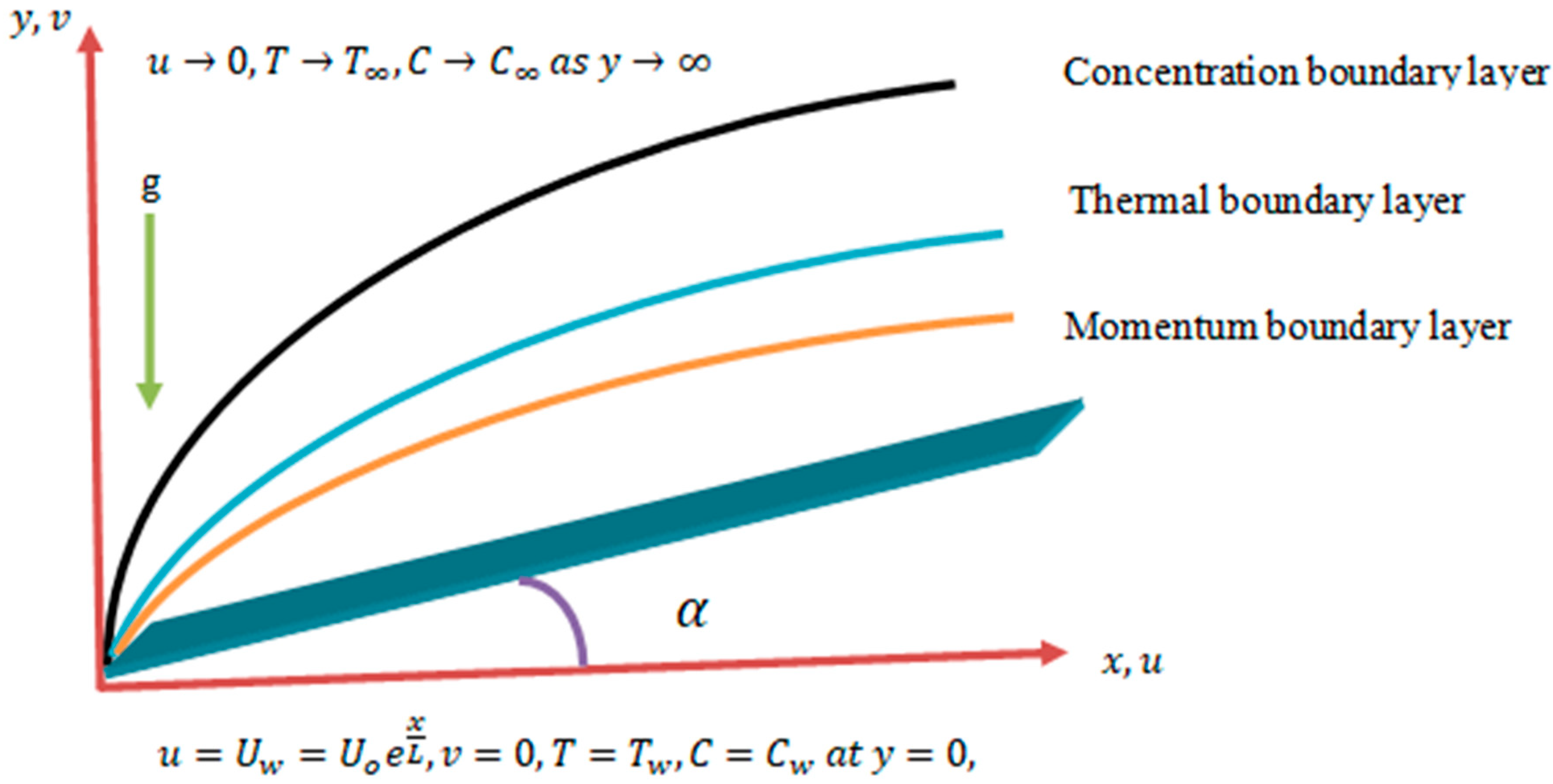
2. Formulation of the Problem

By following [2], Cauchy stress for third grade fluid is given as below;

$$\mathit{T}=-p\mathit{I}+\mu {\mathit{A}}_{\mathbf{1}}+{\alpha }_1{\mathit{A}}_{\mathbf{2}}+{\alpha }_2{\mathit{A}}_{\mathbf{1}}^{\mathbf{2}}+{\beta }_1{\mathit{A}}_{\mathbf{3}}+{\beta }_2\left({\mathit{A}}_{\mathbf{1}}{\mathit{A}}_{\mathbf{2}}+{\mathit{A}}_{\mathbf{2}}{\mathit{A}}_{\mathbf{1}}\right)+{\beta }_3\left(tr{\mathit{A}}_{\mathbf{1}}^{\mathbf{2}}\right){\mathit{A}}_{\mathbf{1}}.$$

(1)

Here, material moduli are ${\alpha }_i$ and ${\beta }_i$. Due to incompressibility constraint spherical stress is $–p\mathit{I}$ in Equation (1), and $\mu$ is dynamic viscosity. Designations ${\mathit{A}}_{\mathbf{1}}$; ${\mathit{A}}_{\mathbf{2}}$ and ${\mathit{A}}_{\mathbf{3}}$ are called kinematical tensors and are defined by

$$\begin{array}{c}{\mathit{A}}_{\mathbf{1}}=\left(\mathbf{\nabla }\mathit{V}\right)+{\left(\mathbf{\nabla }\mathit{V}\right)}^T,\\ {\mathit{A}}_{\mathit{n}}=\frac{d{\mathit{A}}_{\mathit{n}-\mathbf{1}}}{dt}+{\mathit{A}}_{\mathit{n}-\mathbf{1}}\left(\mathbf{\nabla }\mathit{V}\right)+{\left(\mathbf{\nabla }\mathit{V}\right)}^T{\mathit{A}}_{\mathit{n}-\mathbf{1}}\end{array},n=2,3\}$$

(2)

Here, $\frac{d}{dt}$ is material time derivative. The symbols $\mathbf{\nabla }$ and $\mathit{V}$ represent the gradient operator and velocity vector field, respectively. If fluid motion is compatible with thermodynamics and Helmholtz free energy is small at the rest position of fluid, then

$$\begin{array}{c}\begin{array}{c}\mu \ge 0,\\ {\alpha }_1\ge 0, \left|{\alpha }_1+{\alpha }_2\right|\le \sqrt{24\mu {\beta }_3}\end{array},\\ {\beta }_1={\beta }_2=0,{\beta }_3\ge 0.\end{array}\}$$

(3)

Then Equation (1) obtains the following form

$$\mathit{T}=-p\mathit{I}+\mu {\mathit{A}}_{\mathbf{1}}+{\alpha }_1{\mathit{A}}_{\mathbf{2}}+{\alpha }_2{\mathit{A}}_{\mathbf{1}}^{\mathbf{2}}+{\beta }_3\left(tr{\mathit{A}}_{\mathbf{1}}^{\mathbf{2}}\right){\mathit{A}}_{\mathbf{1}}$$

(4)

Flow Analysis

Consider viscous, steady, incompressible, and two-dimensional flow of an electrically conducting third-grade fluid past inclined and exponentially stretching sheet embedded in the porous medium. $B\left(x\right)=B_o{e}^{x/L}$ is the applied magnetic field in $y$-direction. The Darcy–Forchheimer relation is accomplished. Surface temperature is $T_w$, ambient temperature is $T_{\infty }$ with condition $T_w>T_{\infty }$. Surface mass concentration is $C_w$, ambient concentration is $C_{\infty }$ with condition $C_w>C_{\infty }$. The vertical and horizontal coordinates are $x, y$, and the corresponding velocity components are $u,v$ respectively. The flow configuration is depicted in Figure 1.

By following [2,26] the flow equations are given below:

$$\frac{\partial u}{\partial x}+\frac{\partial v}{\partial y}=0$$

(5)

$$\begin{gathered} u\frac{\partial u}{\partial x}+v\frac{\partial u}{\partial y}=\nu \frac{{\partial }^{2}u}{\partial y^2}+\frac{{\alpha }_1}{\rho }\left(u\frac{{\partial }^{3}u}{\partial x\partial y^2}+\frac{\partial u}{\partial x}\frac{{\partial }^{2}u}{\partial y^2}+3\frac{\partial u}{\partial y}\frac{{\partial }^{2}v}{\partial y^2}+\nu \frac{{\partial }^{3}u}{\partial y^3}\right)+2\frac{{\alpha }_2}{\rho }\frac{\partial u}{\partial y}\frac{{\partial }^{2}v}{\partial y^2} \\ +6\frac{{\beta }_3}{\rho }\left(\frac{\partial u}{\partial y}\right){\frac{{\partial }^{2}u}{\partial y^2}}^2+g{\beta }_T\left(T-T_{\infty }\right)cos\alpha +g{\beta }_C\left(C-C_{\infty }\right)cos\alpha -\frac{\sigma B^2\left(x\right)}{\rho }u-\frac{\nu u}{K_o}-F{u}^2 \end{gathered}$$

(6)

$$u\frac{\partial T}{\partial x}+v\frac{\partial T}{\partial y}={\alpha }_m\frac{{\partial }^{2}T}{\partial y^2}$$

(7)

$$u\frac{\partial C}{\partial x}+v\frac{\partial C}{\partial y}=D_m\frac{{\partial }^{2}C}{\partial y^2}$$

(8)

The molded conditions are

$$\begin{array}{c}u=U_w, v=0 ,T=T_w\left(x\right), C=C_w\left(x\right)aty=0,\\ u\to 0 T\to T_{\infty }, C\to C_{\infty } as y\to \infty .\end{array}\}$$

(9)

Here, $U_w=U_o{e}^{\frac{x}{L}}$, stretching velocity, $T_w=T_{\infty }+C_o{e}^{x/L}$ is the wall temperature, and $C_w=C_{\infty }+C_o{e}^{x/L}$ is the wall concentration. Reference velocity, concentration, and temperature are $U_o,C_o$, and $T_o$. Here, ${\beta }_T$, $k$, $\sigma$, ${\beta }_C$, $\nu$, $C_s$, and $\mu$, are coefficient of thermal expansion, thermal conductivity, electrical conductivity, coefficient of concentration expansion, kinematic viscosity, concentration susceptibility, and dynamic viscosity, respectively. Designations$\alpha$, $F=\frac{C_b}{\sqrt{K_o}}$,$C_P$, $C_b$, $D_m$, and $K_o$ are thermal-diffusivity, coefficient of inertia, specific heat at constant pressure, drag coefficient, mass-diffusivity, and permeability of porous medium, respectively. Here, $({\alpha }_1, {\alpha }_2, {\beta }_{3)}$ are material moduli.

3. Solution Methodology

The whole solution methodology for solving the flow equations given in Equations (5)–(8) with boundary conditions is detailed here (9). The entire solution process is outlined here.

3.1. Similarity Formulation

Equations (5)–(9) are nonlinear partial differential equations that are difficult to solve, we first convert them into ordinary differential equations by utilizing variables given in Equation (10) used by [27].

$$\begin{gathered} u=U_o{e}^{\frac{x}{L}}, v=\sqrt{\frac{\nu U_o}{2L}}\left(f\left(\eta \right)+\eta f^{\prime }\left(\eta \right)\right)e^{\frac{x}{L}}, T=T_{\infty }+C_o\theta e^{\frac{x}{L}},C=C_{\infty }+C_o\varphi e^{\frac{x}{L}}, \\ \eta =\sqrt{\frac{U_o}{2L\nu }}y{e}^{x/L} \end{gathered}$$

(10)

The Equation (5) is automatically satisfied when the above-mentioned similarity variables are used in Equation (10), and the Equations (6)–(8) with boundary conditions Equation (9) take the following form.

$$\begin{gathered} f^{‴}+f{f}^{″}-2f^{{\prime }^2}+2Ri\left(\theta +N\varphi \right)cos\alpha +K\left(6f^{\prime }{f}^{‴}-f{f}^{\left(iv\right)}-2\eta f^{″}{f}^{‴}-9f^{″}{}^2\right) \\ -L\left(3f^{″}{}^2+\eta f^{″}{f}^{‴}\right)+3\beta Re{f}^{″}{}^2{f}^{‴}-M{f}^{\prime }-K^{*}{f}^{\prime }-Fr{f}^{{\prime }^2}=0 \end{gathered}$$

(11)

$$f^{\prime }\theta -f{\theta }^{\prime }=\frac{1}{Pr}{\theta }^{″}$$

(12)

$$f^{\prime }\varphi -f{\varphi }^{\prime }=\frac{1}{S_C}\varphi$$

(13)

Boundary conditions

$$\begin{gathered} f=0, f^{\prime }=1 , \theta =1, \varphi =1 as \eta \to 0 \\ {f}^{\prime }\to 1,f^{″}\to 0 , \theta \to 0, \varphi \to 0 as \eta \to \infty . \end{gathered}$$

(14)

Here, $M=\frac{2\sigma B_o^{2}L}{\rho U_o}$ is called the magnetic field parameter, $Fr=\frac{C_{b}L{e}^{\frac{x}{L}}}{\sqrt{K_o}}$ is called local inertial coefficient, $\beta =\frac{{\beta }_3{U}_o{e}^{\frac{x}{L}}}{\rho \nu L}$ is known as the third-grade fluid parameter, $N=\frac{{\beta }_C{C}_o}{{\beta }_T{T}_o},$is termed as buoyancy ratio parameter, $L=\frac{{\alpha }_2{U}_o{e}^{\frac{x}{L}}}{\rho \nu L}$ is called cross- viscous parameter, $Pr$ = $\frac{\nu }{{\alpha }_m}$ represents Prandtl number, $Ri=\frac{Gr}{R{e}^2}$ is called Richardson number, $Re=\frac{U_{o}L}{\nu }$ a is Reynolds number, $K=\frac{{\alpha }_1{U}_o{e}^{\frac{x}{L}}}{2\rho \nu L}$ is viscoelastic parameter, $Gr=\frac{g{\beta }_T\left(T_w-T_{\infty }\right)L^3}{{\nu }^2}$ is called Grashof number, $Sc$=$\frac{\nu }{D_m}$ is Schmidt number, and $K^{*}=\frac{2\nu L}{K_o{U}_o{e}^{\frac{x}{L}}}$ is permeability parameter, and here, the prime notation is the differentiation w.r.t to $\eta$.

The mathematical expressions for the skin friction coefficient, the Nusselt number, and Sherwood number are

$$C_f=\frac{{\tau }_w}{\rho U_w^2}, Nu=\frac{q_{w}x}{k\left(T-T_{\infty }\right)}, Sh=\frac{q_{m}x}{D_m\left(C-C_{\infty }\right)}$$

(15)

where

$$\begin{gathered} {\tau }_w=\left(\frac{\partial u}{\partial y}+\frac{{\alpha }_1}{\mu }\left(2\frac{\partial u}{\partial x}\frac{\partial u}{\partial y}+v\frac{{\partial }^{2}u}{\partial y^2}+u\frac{{\partial }^{2}u}{\partial x\partial y}\right)+\frac{2{\beta }_3}{\mu }{\left(\frac{\partial u}{\partial y}\right)}^2\right) \\ {q}_w=-k\left(\frac{\partial T}{\partial y}\right), q_m=-D_m\left(\frac{\partial C}{\partial y}\right) \\ \mathrm{at} y=0. \end{gathered}$$

(16)

are stress tensor, heat and mass flux at surfaces, respectively. The transformed form is Equations (15) and (16), which are given as follows:

$$\begin{array}{c}{C}_f=\frac{2}{\sqrt{Re}}\left[f^{″}\left(0\right)+K\left(3f^{\prime }\left(0\right)f^{″}\left(0\right)-f\left(0\right)f^{″}\left(0\right)\right)+2\beta Re{f}^{″}{}^2\left(0\right)\right],\\ R{e}^{-1/2}Nu=-\theta \prime \left(0\right),\\ R{e}^{-1/2}Sh=-\varphi \prime \left(0\right),\end{array}\}$$

(17)

3.2. Solution Technique

Approximate solutions of the Equations (11)–(14) are determined by MALAB built-in Numerical Solver bvp4c. Pertinent parameters are local inertial coefficient $Fr$, third-grade fluid parameter $\beta$, buoyancy ratio parameter $N$, cross- viscous parameter $L$, Prandtl number $Pr$, viscoelastic parameter $K$, Schmidt number $Sc$, permeability parameter $K^{*}$, and magnetic field parameter $M$. The numerical results of the considered model are determined with the use of MALAB built-in Numerical Solver bvp4c. Equations (11)–(14) are transformed to first order ODEs and then put to bvp4c for solutions. Equations are set,

$$f=y\left(1\right), f^{\prime }=y\left(2\right),f^{″}=y\left(3\right), f^{‴}=y\left(4\right),\theta =y\left(5\right), {\theta }^{\prime }=y\left(6\right), \varphi =y\left(7\right),{\varphi }^{\prime }=y\left(8\right),$$

(18)

$$\begin{array}{ll}{f}^{\left(iv\right)}=yy1=& (1/K\ast y\left(1\right))\ast (2\ast Ri\ast \left(N\ast y\left(7\right)+y\left(5\right)\right)\ast \cos \alpha +y\left(4\right)+y\left(1\right)\ast y\left(3\right)-2\ast y{\left(2\right)}^2+K\\ & \ast (6\ast y\left(2\right)\ast y\left(4\right)-2\ast \eta \ast y\left(3\right)\ast y\left(4\right)-9\ast y{\left(3\right)}^2)-L\ast \left(3\ast y{\left(3\right)}^2+\eta \ast y\left(2\right)\ast y\left(4\right)\right)+3\\ & \ast \beta \ast Re\ast y{\left(3\right)}^2\ast y\left(4\right)-y\left(2\right)\ast \left(K^{\ast }+M+y\left(2\right)+Fr\ast y\left(2\right)\right)))\end{array}$$

(19)

$${\theta }^{″}=yy2=Pr\ast \left(y\right(2)\ast y(5)-y(1)\ast y(6\left)\right)$$

(20)

$${\varphi }^{″}=Sc \ast \left(y\right(2)\ast y(7)-y(1)\ast y(8\left)\right))$$

(21)

Boundary conditions’

$$y_o\left(1\right)=0,{ y}_o\left(2\right)=1,{ y}_o\left(5\right)=1,{ y}_o\left(7\right)=1, yinf\left(2\right)=0, yinf\left(3\right)=0, yinf\left(5\right)=0, yinf\left(7\right)=0.$$

(22)

Equations (18)–(22) are solved to get the numerical solutions of velocity profile $f^{\prime }\left(\eta \right)$, temperature profile $\theta \left(\eta \right)$, and mass concentration $\varphi \left(\eta \right)$. Furthermore, the skin friction coefficient $R{e}^{1/2}{C}_f$, Nusselt number $R{e}^{-1/2}Nu$, and Sherwood number $R{e}^{-1/2}Sh$ are graphed and tabulated.

4. Results and Discussion

Now we focus on analyzing and discussing the physical behavior of unknown qualities of interest under the influence of physical parameters found in flow equations. Local inertial coefficient $Fr$, buoyancy ratio parameter $N$, Prandtl number $Pr$, Richardson number $Ri$, viscoelastic parameter $K$, Schmidt number $Sc,$ permeability parameter $K^{*}$, third-grade fluid parameter $\beta$, magnetic field parameter $M$, and cross viscous parameter $L$ effects are estimated onvelocity distribution $f^{\prime }\left(\eta \right)$, temperature distribution $\theta \left(\eta \right)$, concentration profile $\varphi \left(\eta \right)$. Behavior of the skin friction coefficient $R{e}^{1/2}{C}_f$ heat transfer rate coefficient (Nusselt number) $R{e}^{-1/2}Nu$, and mass transfer rate coefficient (Sherwood number) $R{e}^{-1/2}Sh$ under sundry parameters are observed and graphed (see Figure 2, Figure 3, Figure 4, Figure 5, Figure 6, Figure 7, Figure 8, Figure 9, Figure 10, Figure 11, Figure 12, Figure 13, Figure 14, Figure 15, Figure 16, Figure 17, Figure 18, Figure 19, Figure 20, Figure 21, Figure 22, Figure 23, Figure 24, Figure 25, Figure 26 and Figure 27) and tabulated. The present results are compared with already published results in

Table 1. Comparison of results for $-{\theta }^{\prime }\left(0\right)$ when $Ri=0,N=0,Sc=0,M=0,\beta =0,L=0,K=0,K^{*}=0,Fr=0$.

Pr	Magyari and Keller [31]	Present Study
1.0	0.9547	0.9551
3	1.8691	1.8121
5	2.5001	2.5577
10	3.6604	3.6868

and it is observed that there is good agreement between them. This good agreement ensures the validation of accuracy of the results.

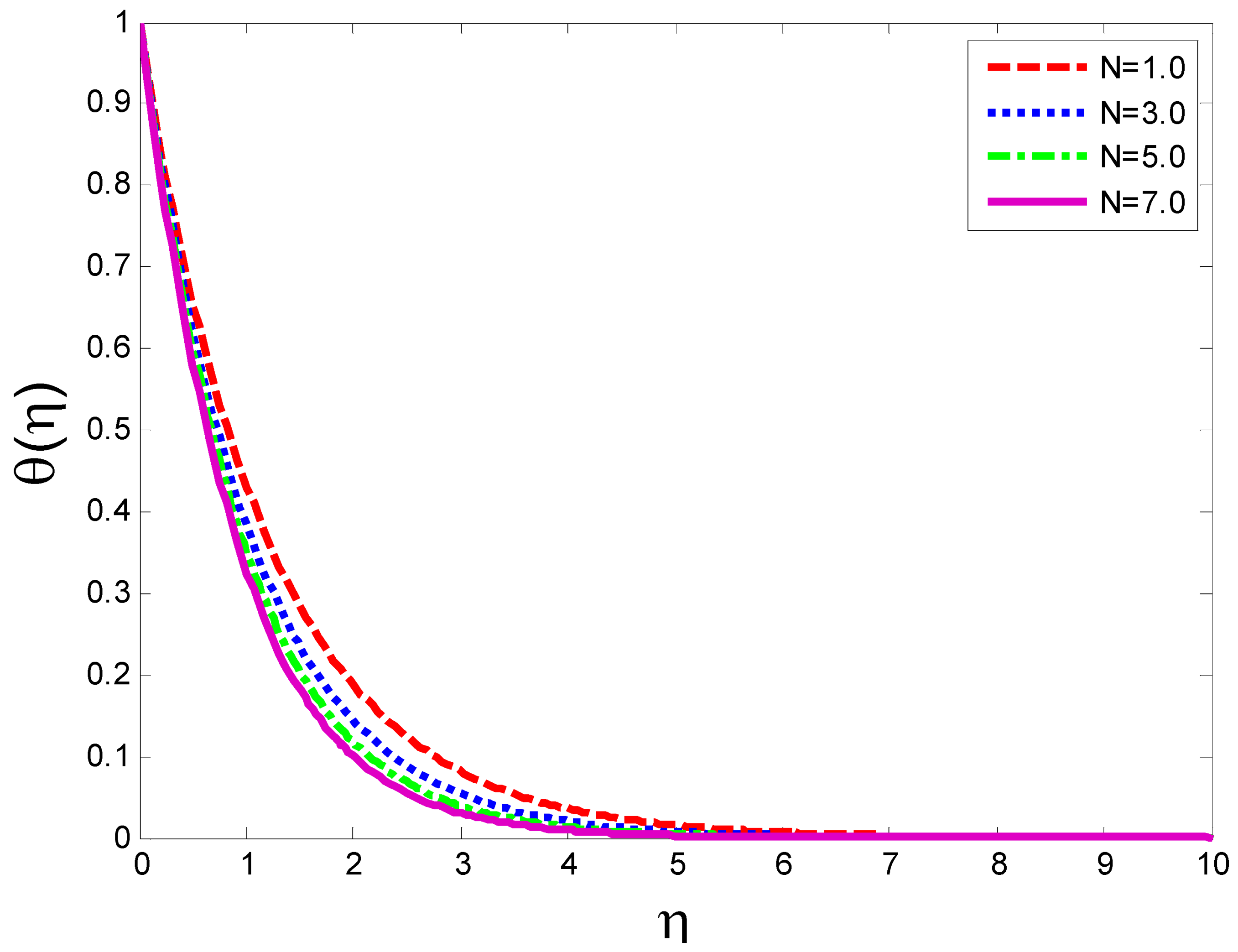
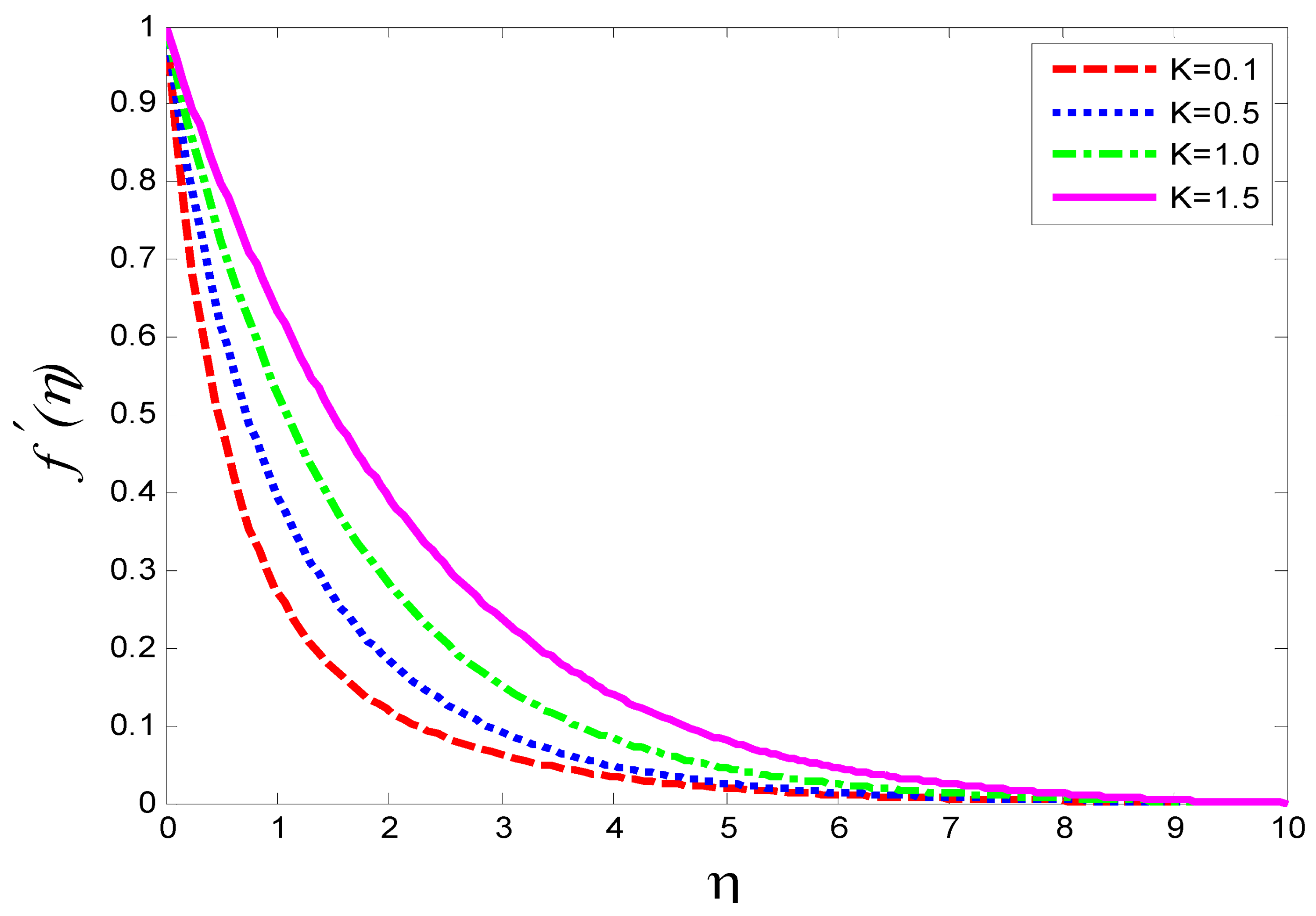
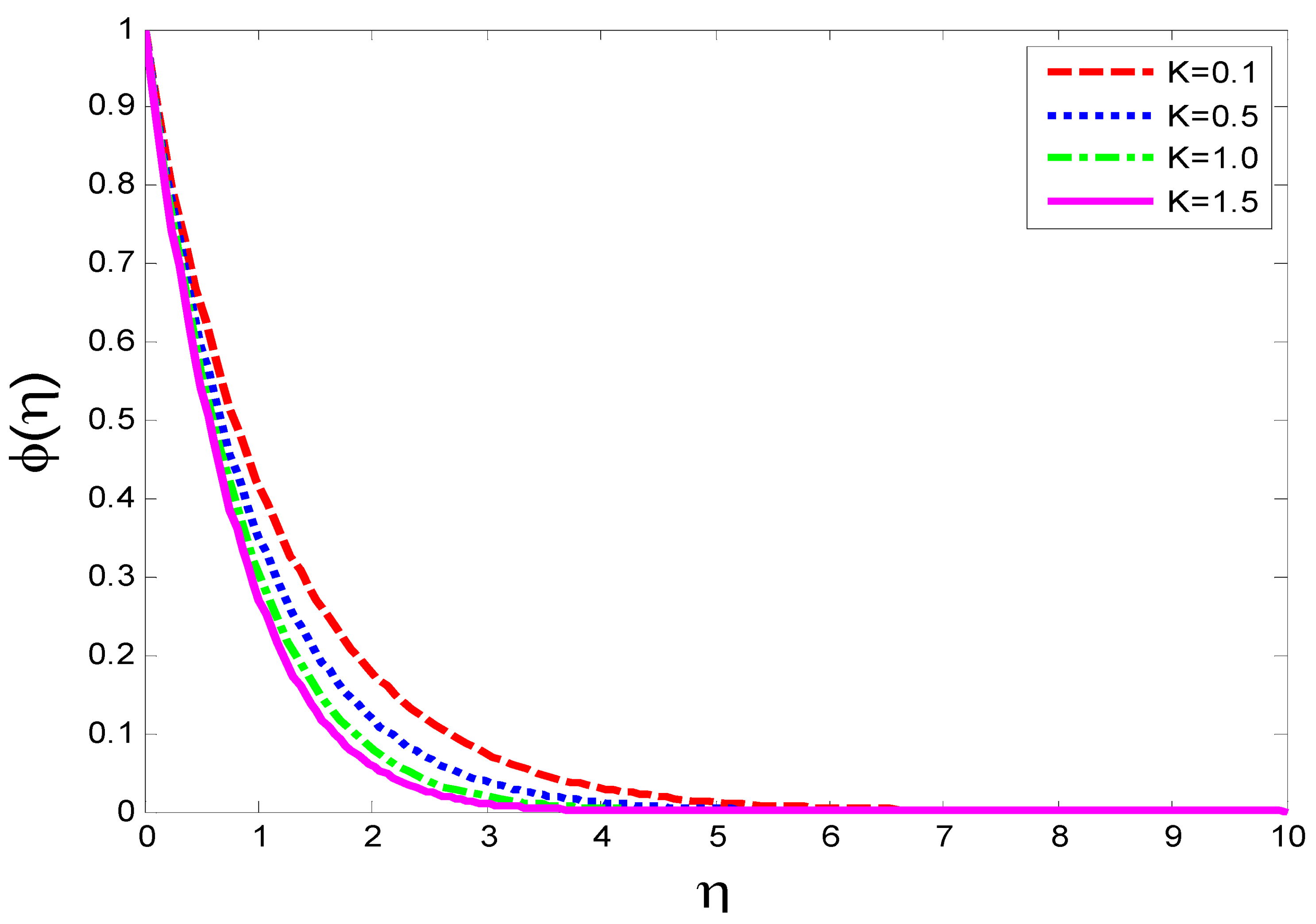
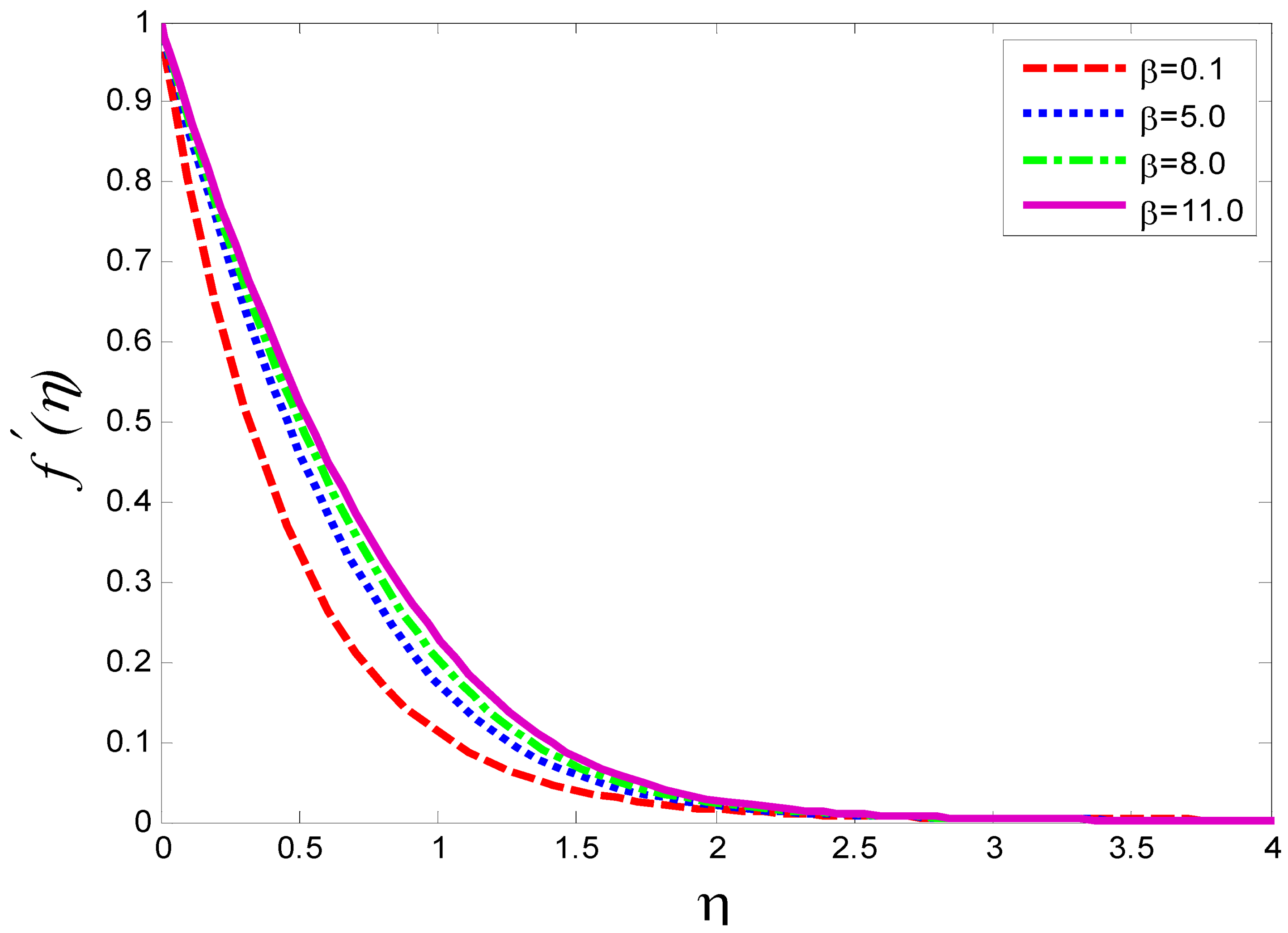
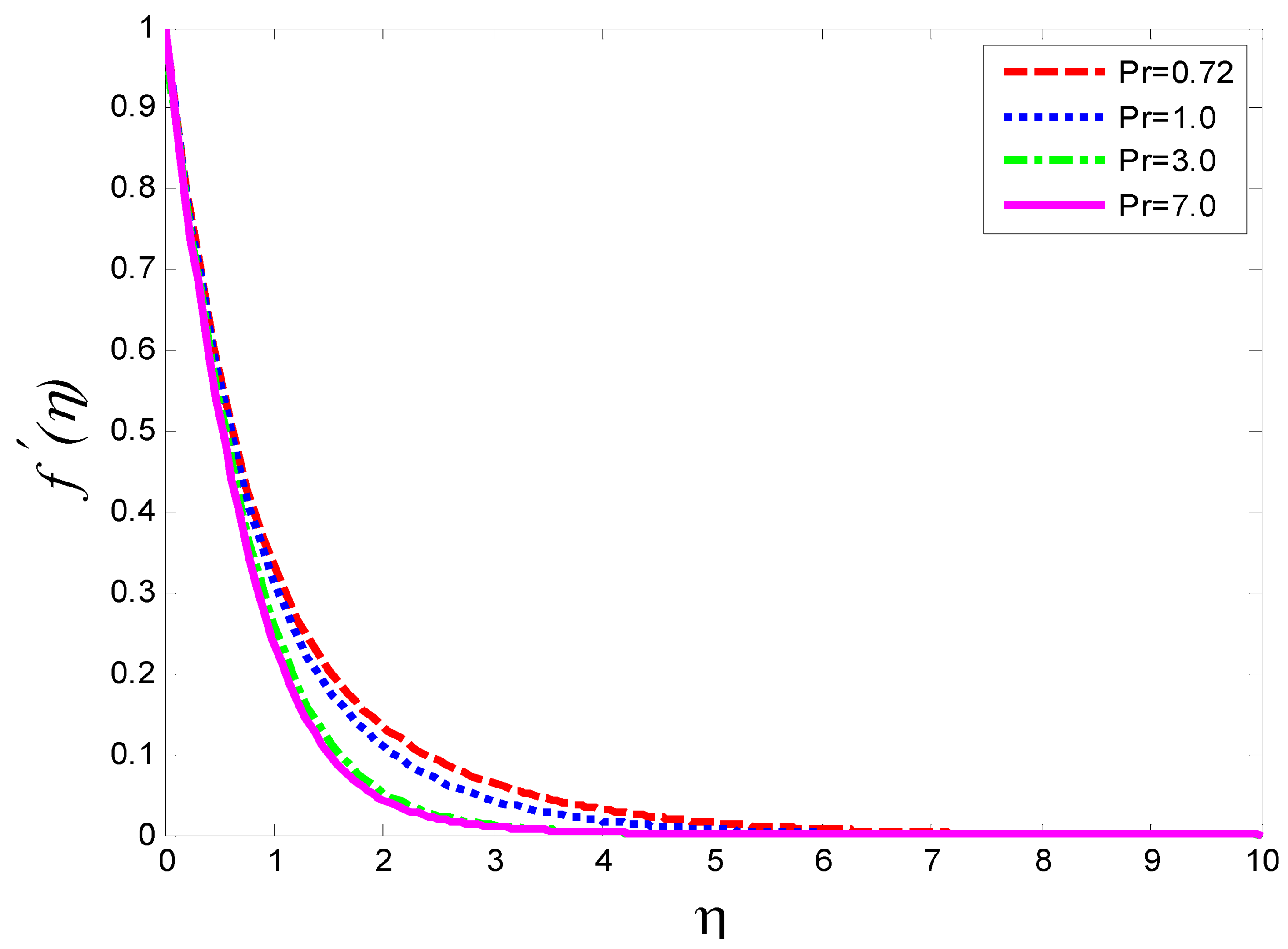
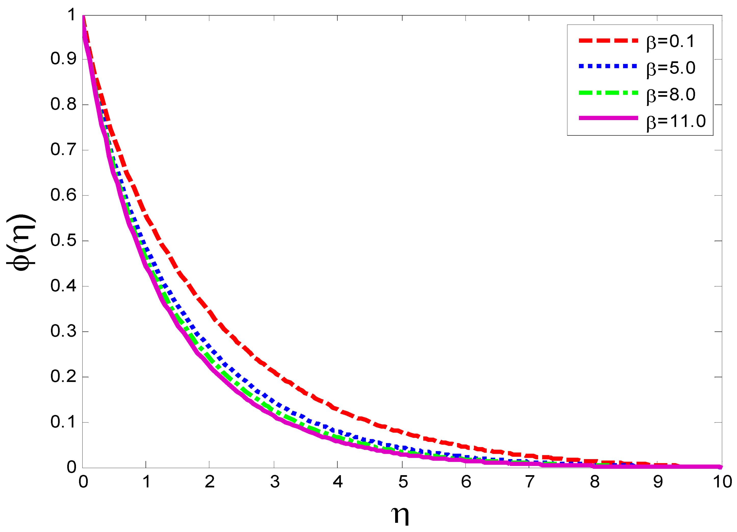
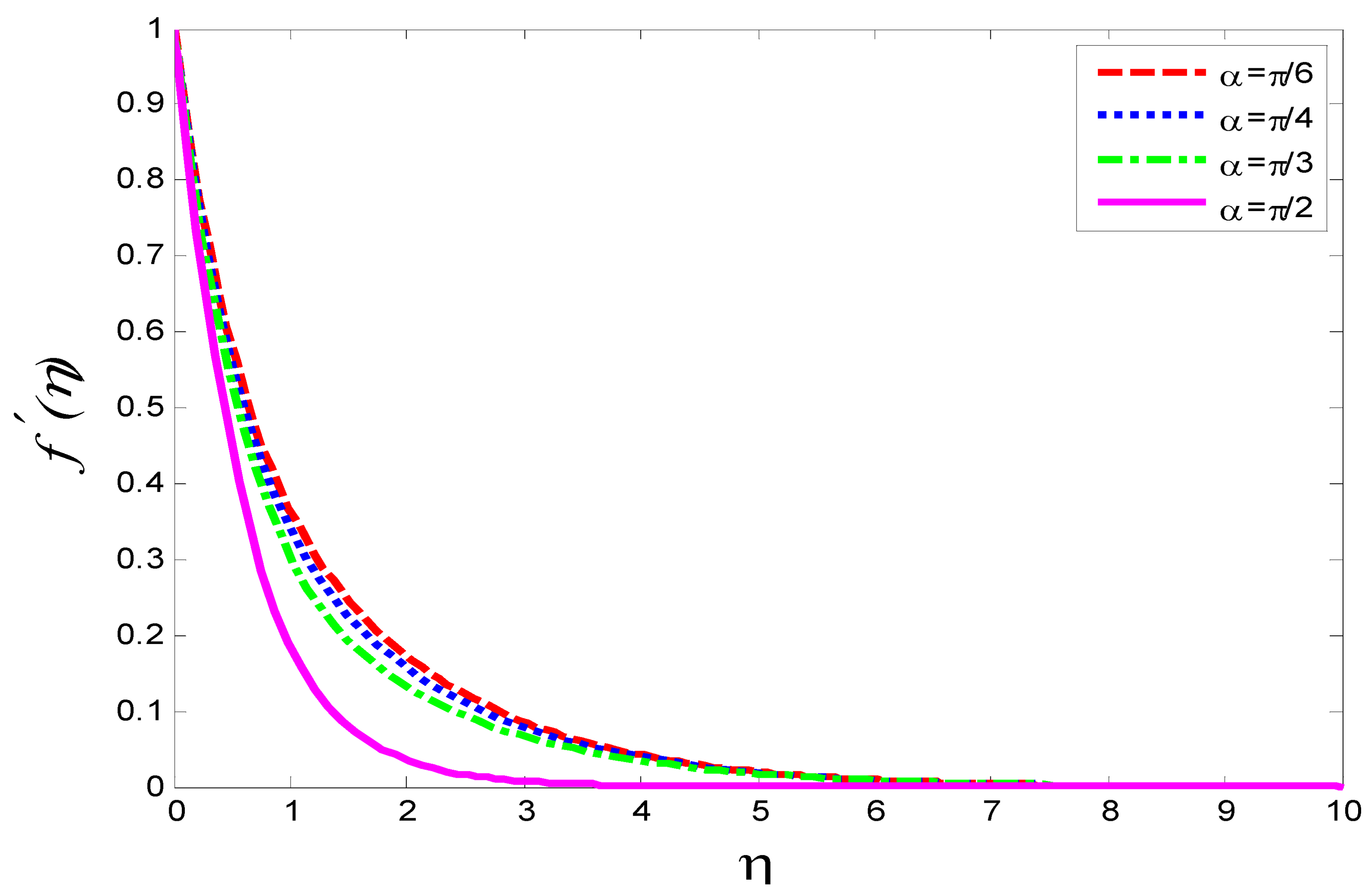
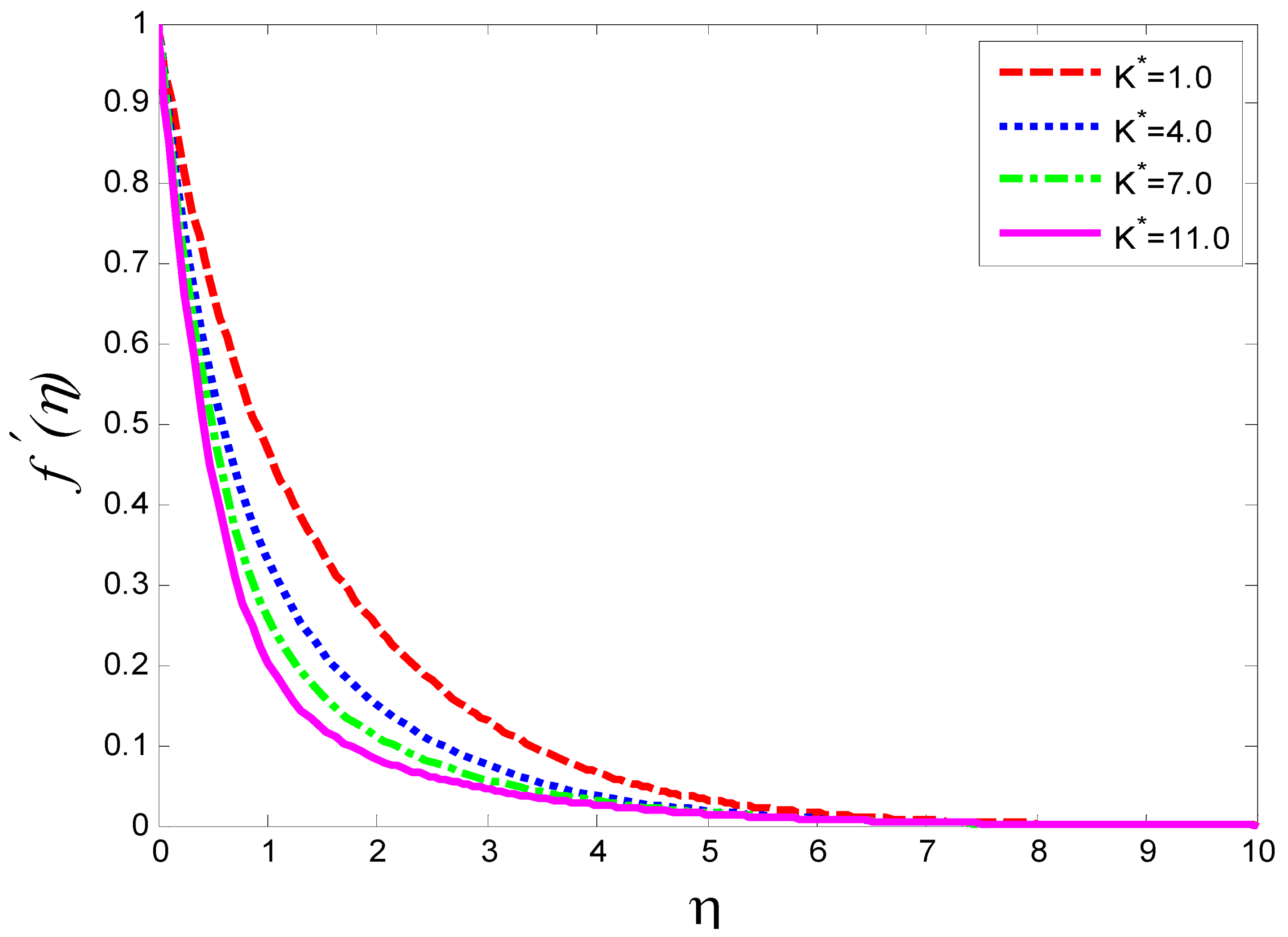
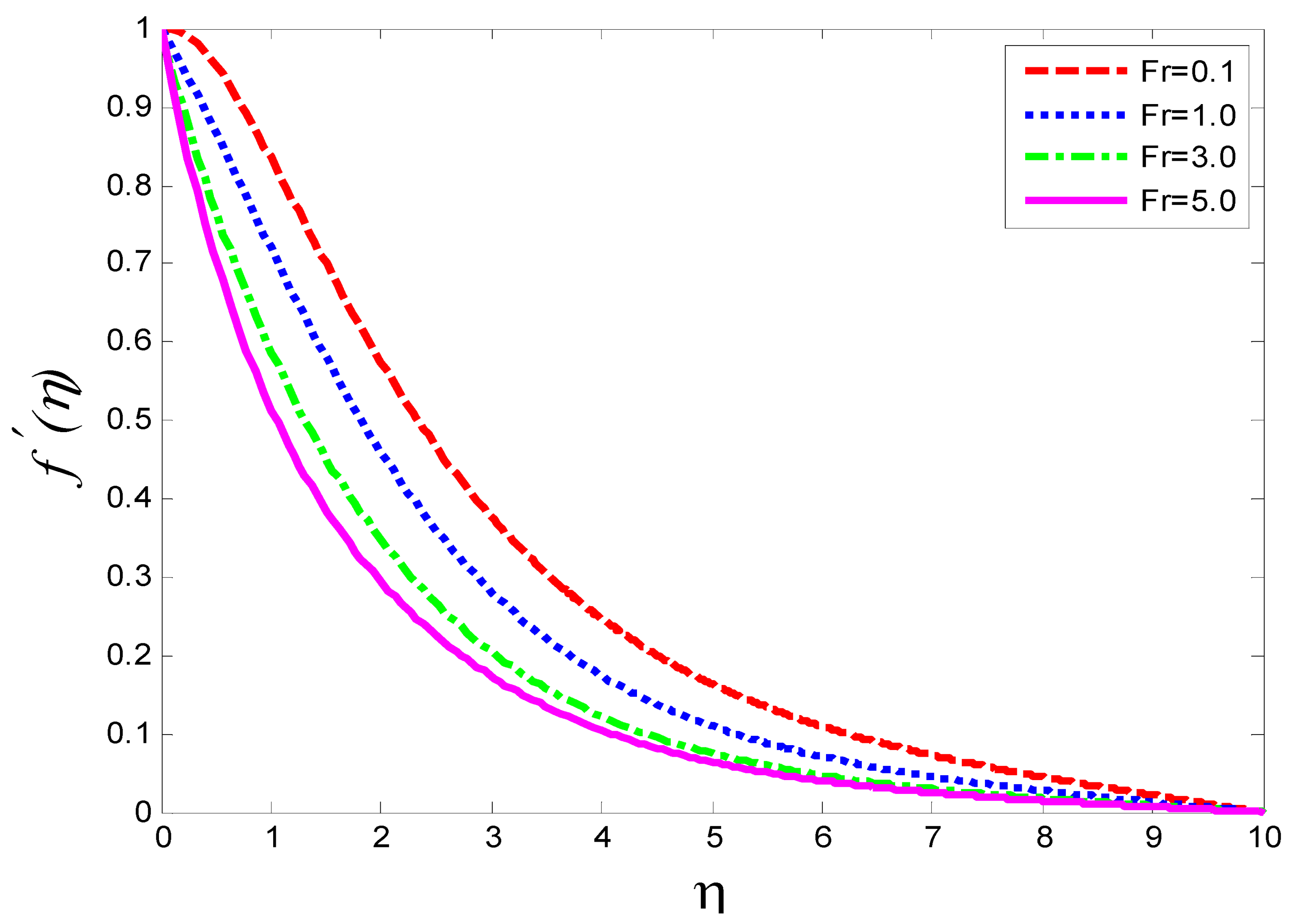
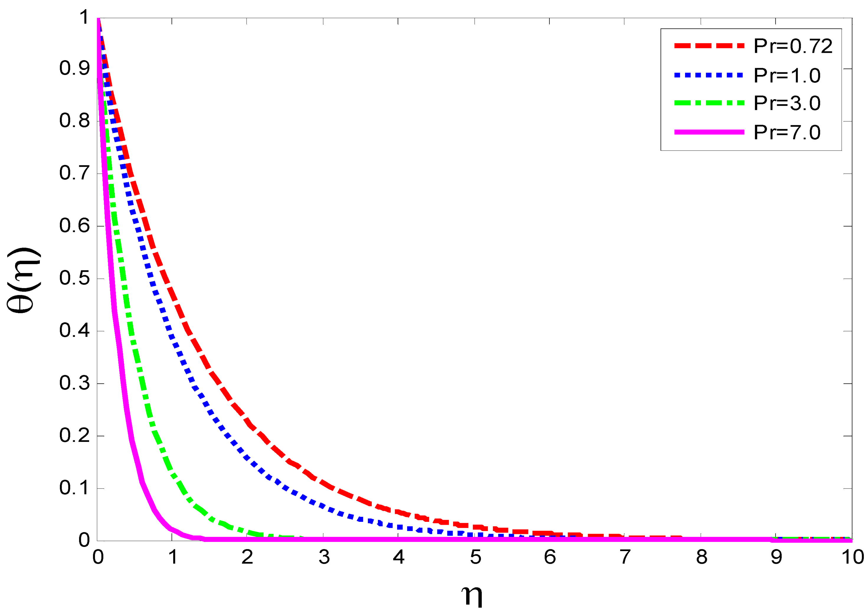
4.1. Influence of Involved Parameters on Velocity Profile $f^{\prime }\left(\eta \right),$ Temperature Profile $\theta \left(\eta \right)$, and Mass Concentration $\varphi \left(\eta \right)$

For elevated values of $Ri$, the physical behavior of $f^{\prime }(\eta$) is shown in Figure 2. Elevation in $Ri$ results in the strong augmentation in $f^{\prime }\left(\eta \right)$, that is to mention that the rest of the material numbers are kept fixed. Here, this is the result of the forced convection effects being minimized and the free convection effects being enhanced, which is due to the velocity of the fluid rising up by a reasonable difference according to the momentum with which the boundary layer thickness increases. Results plotted in Figure 3 are imparting the effects of $N$ on $\theta \left(\eta \right)$. Graphical findings indicate that $\theta \left(\eta \right)$ is decreasing functions of $N$ and leading the reduction in the thermal boundary layer thickness. Figure 4 and Figure 5 portray the variations in profiles of velocity, and concentration against the increasing values of viscoelastic parameter $K$. Findings depict that flow velocity goes on enhancement as shown in Figure 4, but reverse trends in $\varphi$ are seen, as shown in Figure 5. In order to have an insight on the influence of $\beta$ on $f^{\prime }\left(\eta \right)$, $\theta \left(\eta \right)$ and $\varphi \left(\eta \right)$ the Figure 6, Figure 7 and Figure 8 are sketched, respectively. Plots show that augmentation in $\beta$ gives rise in fluid velocity, and a decreasing trend is noted for temperature and concentration profiles. This is due to the fact that as $\beta$ increases, the basic viscosity of the fluid is attenuated, which causes the fluid velocity to increases rapidly. Physical consequences of cross-viscous parameter $L$ on $f^{\prime }\left(\eta \right)$ are shown in Figure 9. It is worth mentioning that when $L$ rises, a decrement in $f^{\prime }\left(\eta \right)$ is noted.

The influence ofangle of inclination $\alpha$ on $f^{\prime }\left(\eta \right)$ is depicted in Figure 10. There is reduction noted in $f^{\prime }\left(\eta \right)$, as angle of inclination $\alpha =\frac{\pi }{6}$ to $\alpha =\frac{\pi }{2}$ as shown in Figure 10. In the case when $\alpha =\pi /2$ the horizontal plate is secured, and in the case when $\alpha =0^0$ a vertical plate is obtained, and for the rest of values of $\alpha$ in between $0<\alpha <\pi /2$ an inclined sheet is retained. In Figure 11 and Figure 12 the impact of permeability parameter $K^{*}$ on $f^{\prime }\left(\eta \right),$ and $\varphi \left(\eta \right)$ is demonstrated, respectively. Figures indicate that increasing values of $K^{*}$ leave the decreasing trend in $f^{\prime }\left(\eta \right)$ and increasing trend in $\varphi \left(\eta \right)$. From the definition of permeability parameter $K^{*}$, it is easy to conclude that as $K^{*}$ is intensified as a result of an increase in viscosity and decrease in porosity of medium, that compels the fluid to slow down in speed. In Figure 13 and Figure 14 the behavior of the velocity field and mass concentration owing to enlarging values of $Fr$is displayed, respectively. Graphs reflect that as $Fr$ is enlarged, velocity drops down, but the temperature field gets stronger at angle $\alpha =\frac{\pi }{6}$. Physically it is endorsed by the fact that an increase in $Fr$ is due to an increase in $C_b$ and a decrease in porosity of medium that causes fluid velocity to fall down. Figure 15 and Figure 16, reveal the physical influence of $Pr$ on velocity distribution and temperature distribution, respectively. Plots show that by raising $Pr$, the velocity and temperature both fall down. From Figure 15 and Figure 16 it is observed that when $Pr$ is increased, velocity and temperature distribution are depleted. The physics of the Prandtl number are endorsed by the above happening. When $Pr$ augments, the viscosity of the fluid gets stronger and the thermal conductance of the fluid gets weaker, thus there is retardation in the speed of fluid and depletion in temperature of the fluid. The effect of the magnetic field parameter $M$ on $f^{\prime }\left(\eta \right)$, and $\theta \left(\eta \right)$ is revealed in Figure 17 and Figure 18, respectively. It is seen that the increment of $M$, $f^{\prime }\left(\eta \right)$, is reduced but $\theta \left(\eta \right)$ are improved. As a result of the application of a magnetic field, Lorentz force is created and hence resistance is produced, so velocity is delineated and temperature is strengthened. All of the graphs are plotted at an angle of $\alpha =\frac{\pi }{6}$ (inclined exponentially stretching sheet), and all of the graphs that satisfy the modeled boundary constraints have asymptotic behavior.

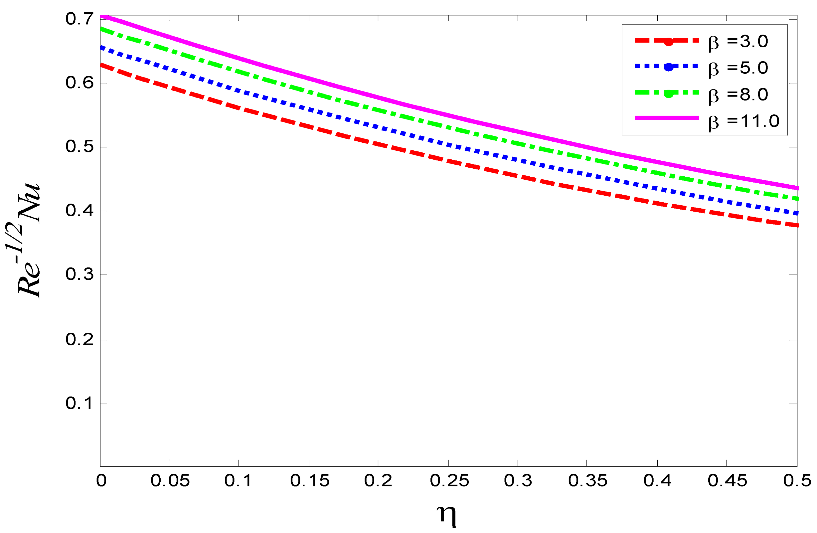
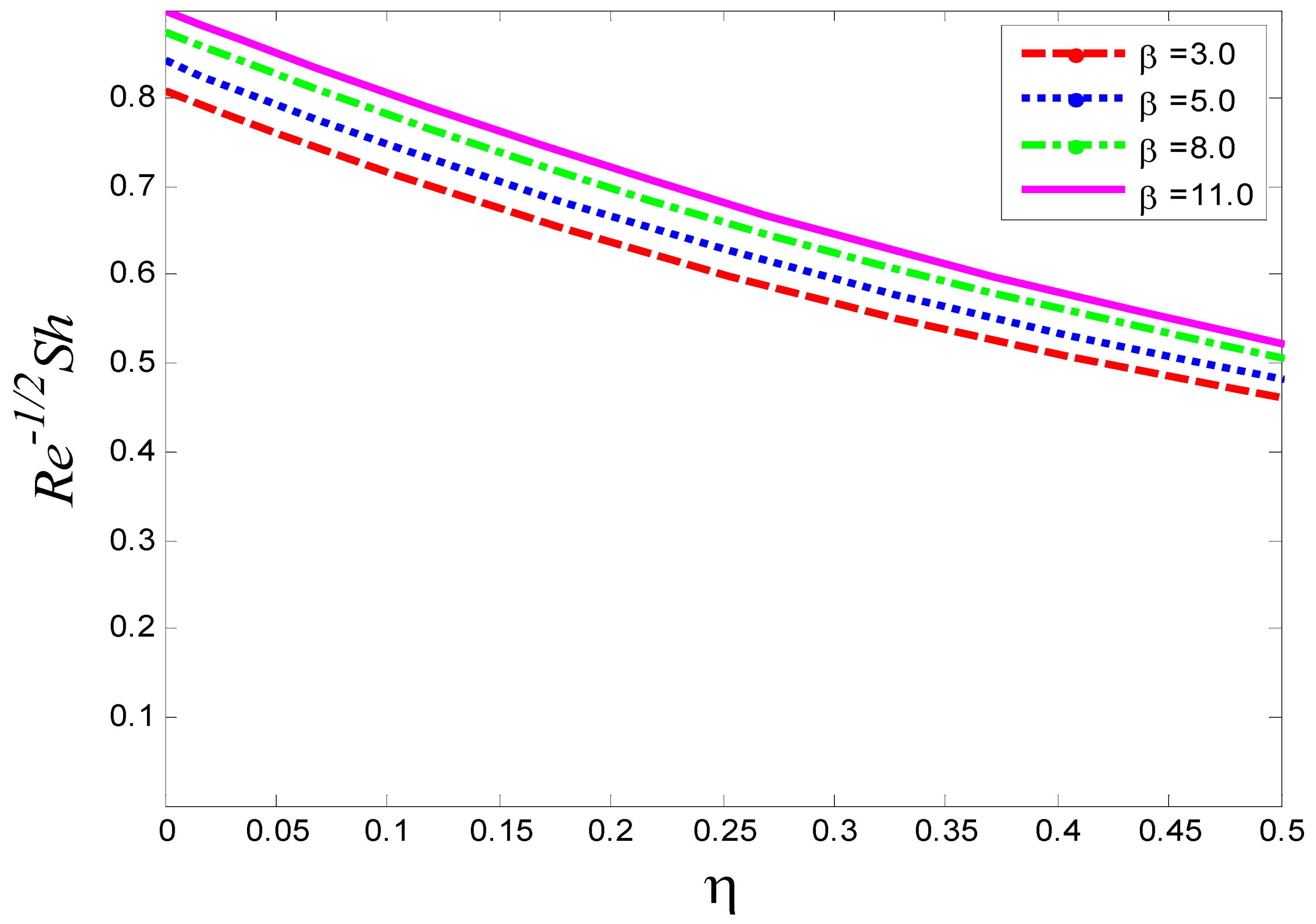
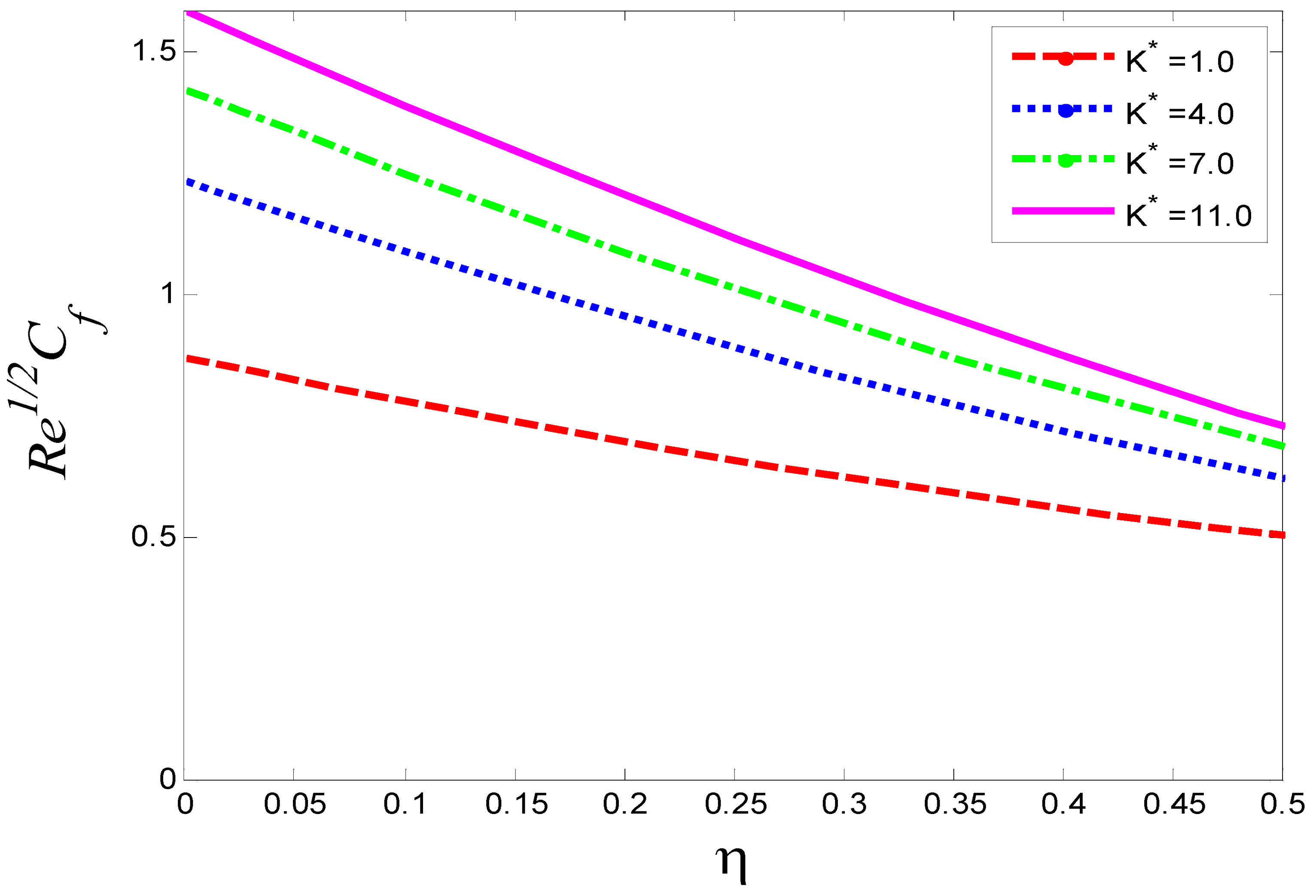
4.2. Influence of Parameters on Skin Friction Coefficient $R{e}^{1/2}{C}_f$, Nusselt Number $R{e}^{-1/2}Nu$, and Sherwood Number $R{e}^{-1/2}Sh$

Here, the influence of third-grade fluid parameter $\beta$, permeability parameter $K^{*}$, and local inertial coefficient on the skin friction coefficient $R{e}^{1/2}{C}_f$, Nusselt number $R{e}^{-1/2}Nu$, and Sherwood number $R{e}^{-1/2}Sh$ are shown in Figure 19, Figure 20, Figure 21, Figure 22, Figure 23, Figure 24, Figure 25, Figure 26 and Figure 27. In Figure 19 the effect of third-grade fluid parameter $\beta$ on the skin friction coefficient $R{e}^{1/2}{C}_f$ is shown. The graph shows that as $\beta$ is increased $R{e}^{1/2}{C}_f$ reduces. Figure 20 depicts the influence of $\beta$ on the Nusselt number $R{e}^{-1/2}Nu$. From the graphical results it is concluded that as $\beta$ is enhanced, then the Nusselt number increases. Figure 21 illustrates the consequences of the third-grade fluid parameter on the Sherwood number $R{e}^{-1/2}Sh$. It can bee seen that there is a direct relation between the Sherwood number and $\beta$. Figure 22, Figure 23 and Figure 24 show the numerical solutions of the skin friction coefficient, Nusselt number and Sherwood number, respectively, under the effect of the permeability parameter $K^{*}$. It is viewed that as $K^{*}$ is augmented, then there is a direct relation between $R{e}^{1/2}{C}_f$ and $K^{*}$ but an inverse relation is seen between $K^{*}$ and the Nusselt number and the Sherwood number. Figure 25, Figure 26 and Figure 27 are plotted to show the physical behavior of the skin friction coefficient, the Nusselt number, and the Sherwood number, respectively, against the different values of local inertial coefficient. From Figure 25, it is noted that as $Fr$ is enhanced, an increment in $R{e}^{1/2}{C}_f$, is observed. Figure 26 and Figure 27 show that as $Fr$ is raised then a reduction in $R{e}^{-1/2}Nu$ and $R{e}^{-1/2}Sh$ is observed. Table 1 shows the comparison of numerical results for $-{\theta }^{\prime }\left(0\right)$ with the numerical results available in the literature for such a special case. Tabular results show good agreement between the already published results and current results, which show the validation of the current algorithm.All these are results presented in Table 1 and Figure 19, Figure 20, Figure 21, Figure 22, Figure 23, Figure 24, Figure 25, Figure 26 and Figure 27 are computed exactly at the surface at angle of inclination$\alpha =\pi /6$.

5. Conclusions

The present study deals with numerical evaluation of third-grade fluid flow and heat transfer with the effect of the Darcy–Forchheimer relation along the inclined exponentially stretching sheet embedded in a porous medium. The equations are solved by MATLAB built-in numerical solver bvp4c. The major outcomes of the current work are as follows:

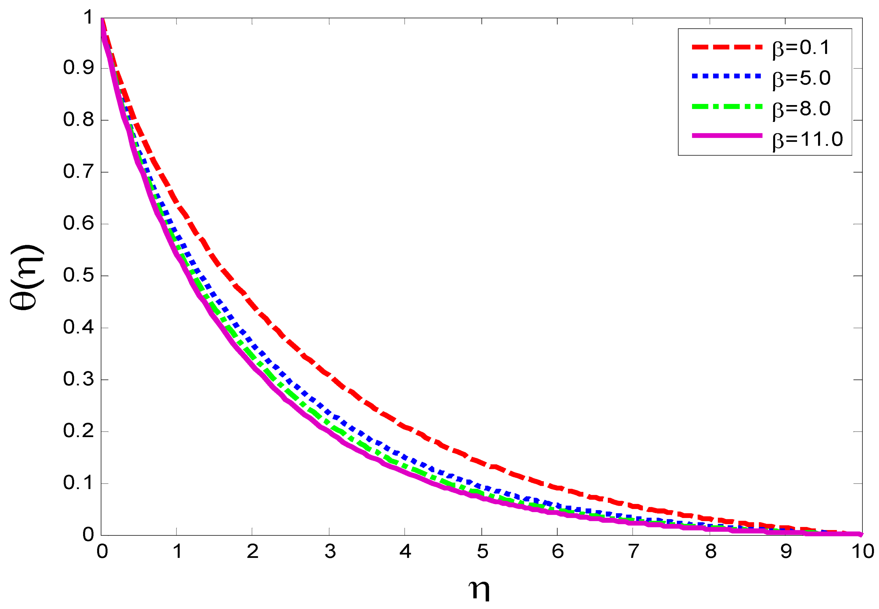
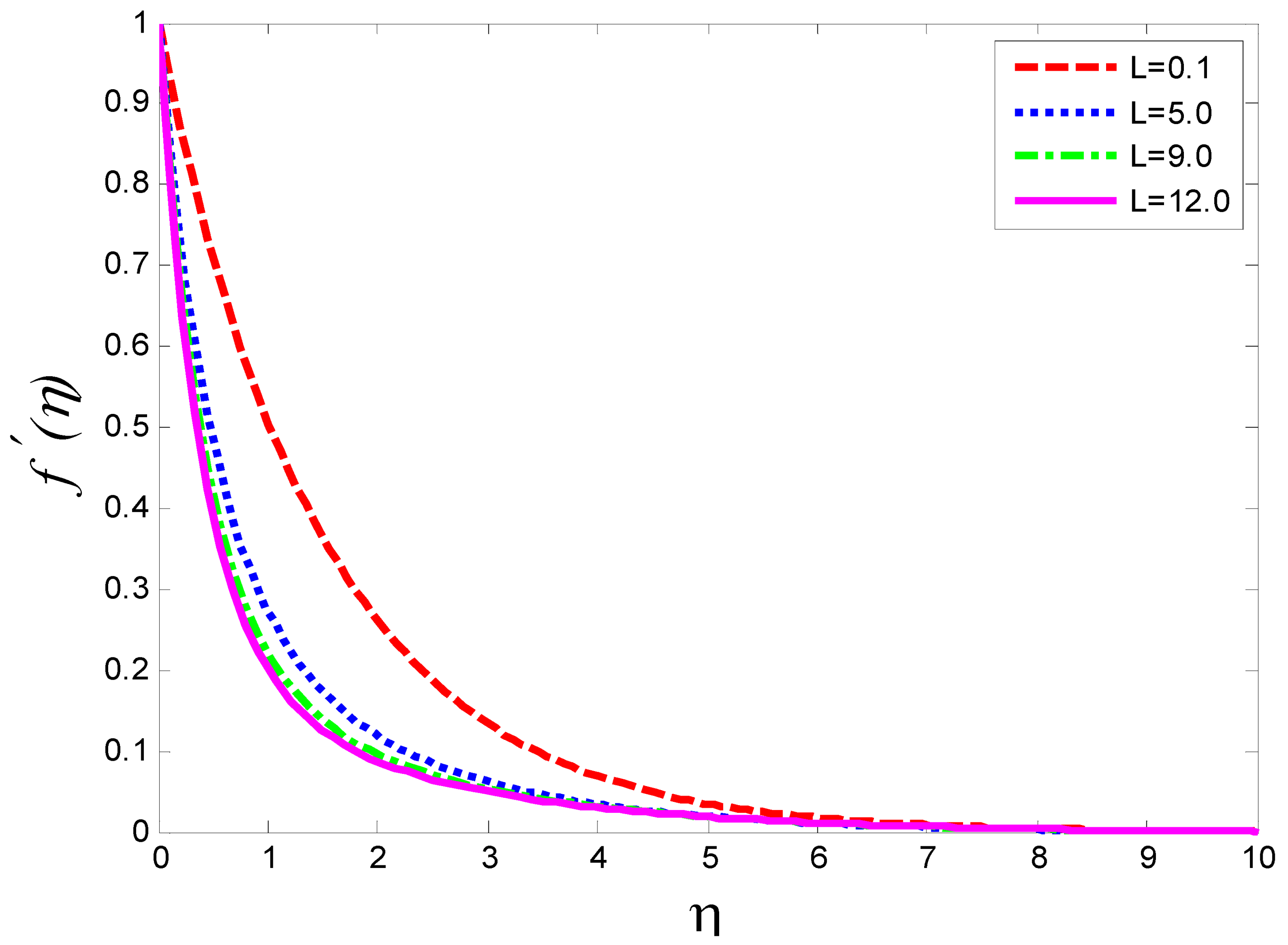
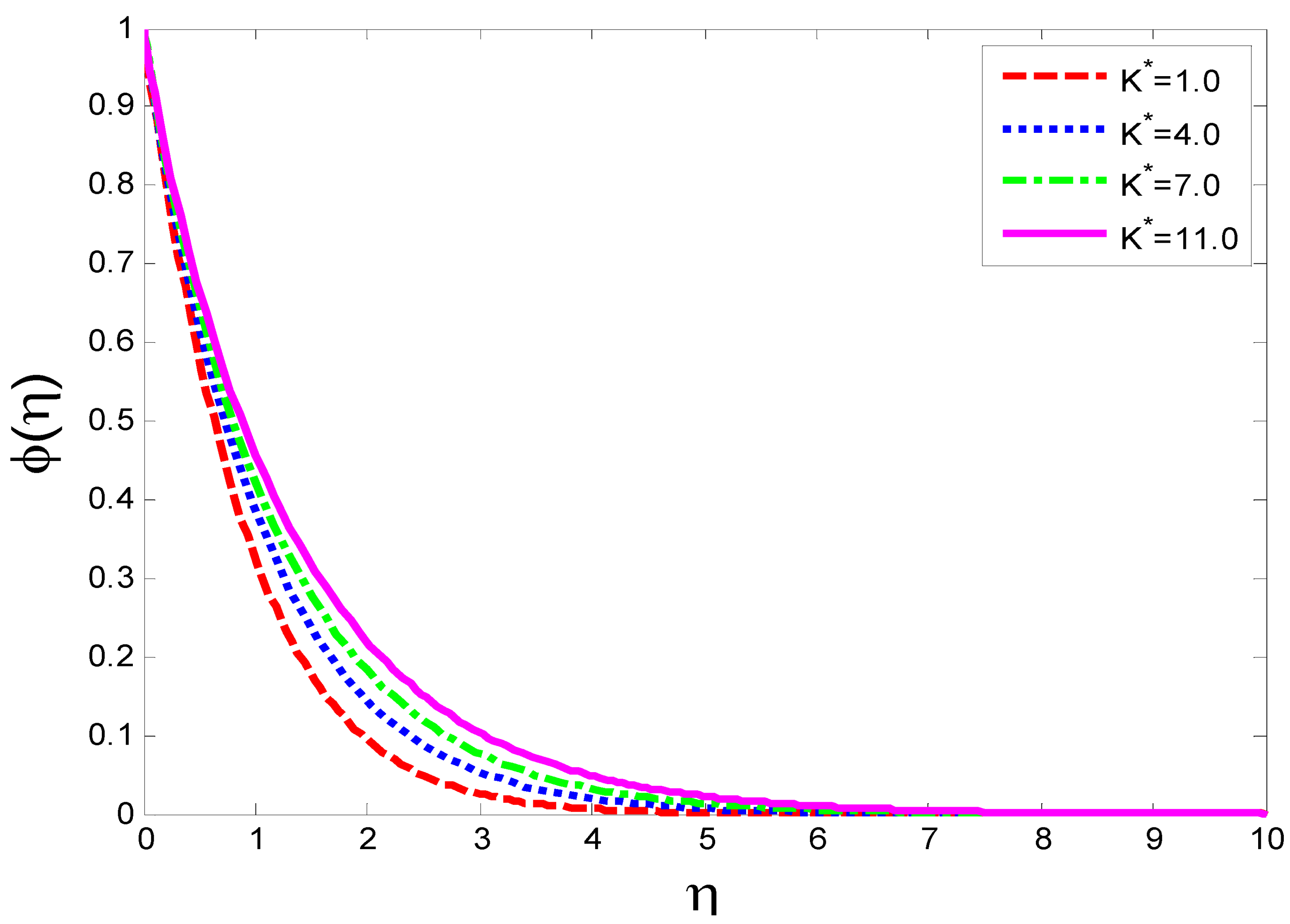
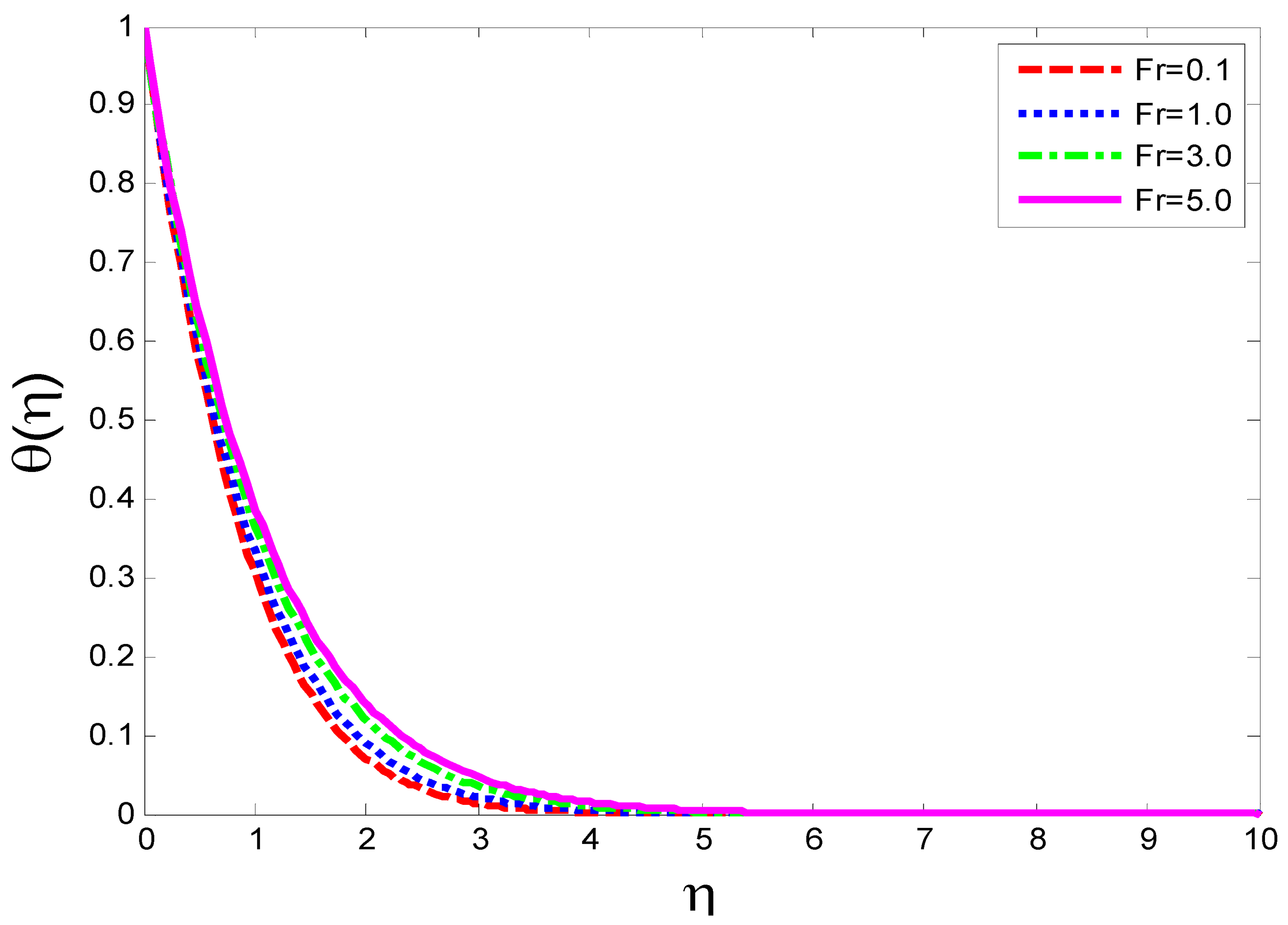
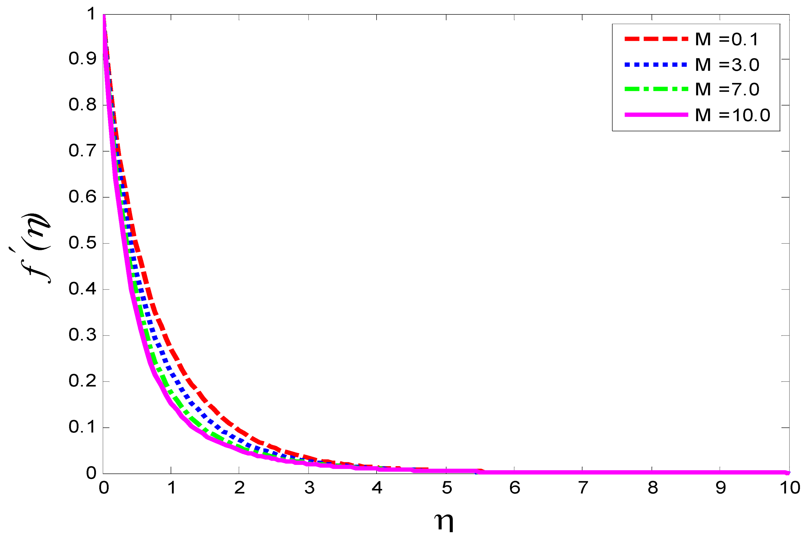
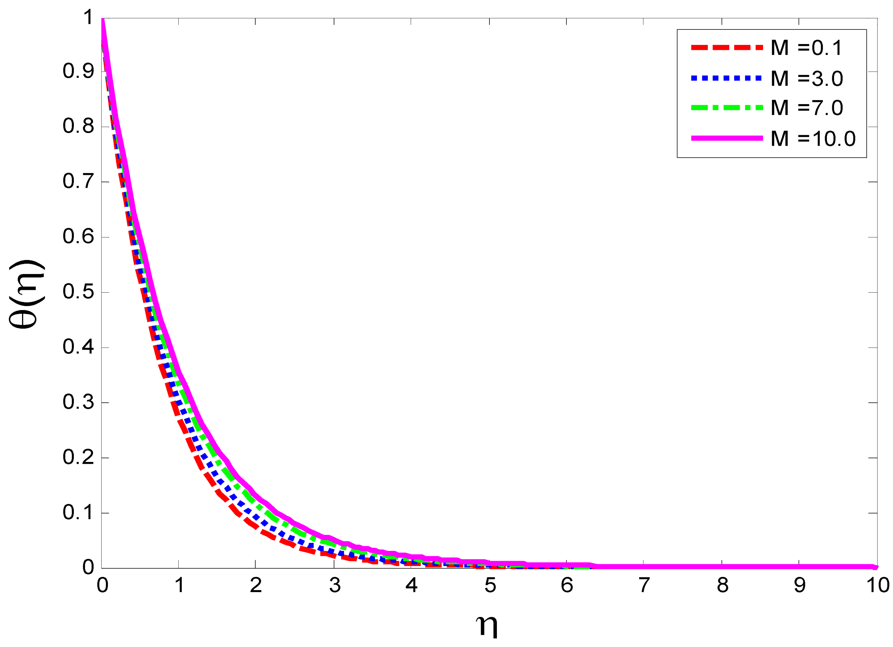
• $f^{\prime }\left(\eta \right)$ rises as $Ri, K$ and $\beta$ rises, but the reverse scenario is noted against the elevating values of $L,K^{*}, Fr,$ and $Pr$.
• $\theta \left(\eta \right)$ is elevated as $N$ and $Fr$ are raised, but the reverse scenario is noted owing to increase in $\beta$ and $Pr$.
• $\varphi \left(\eta \right)$ is intensified as $K^{*}$ is augmented but falls down as $\beta$ and $K$ are elevated.
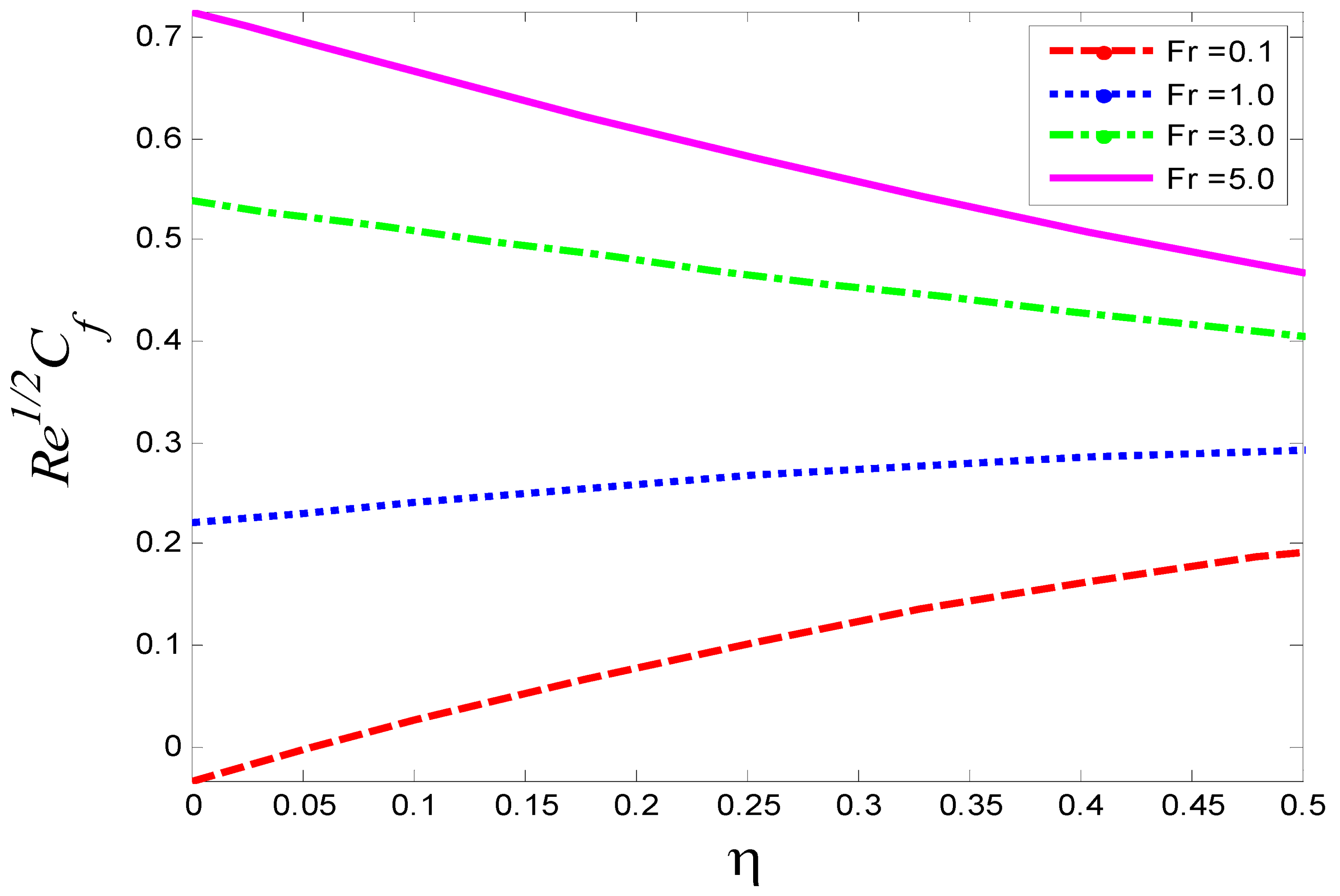
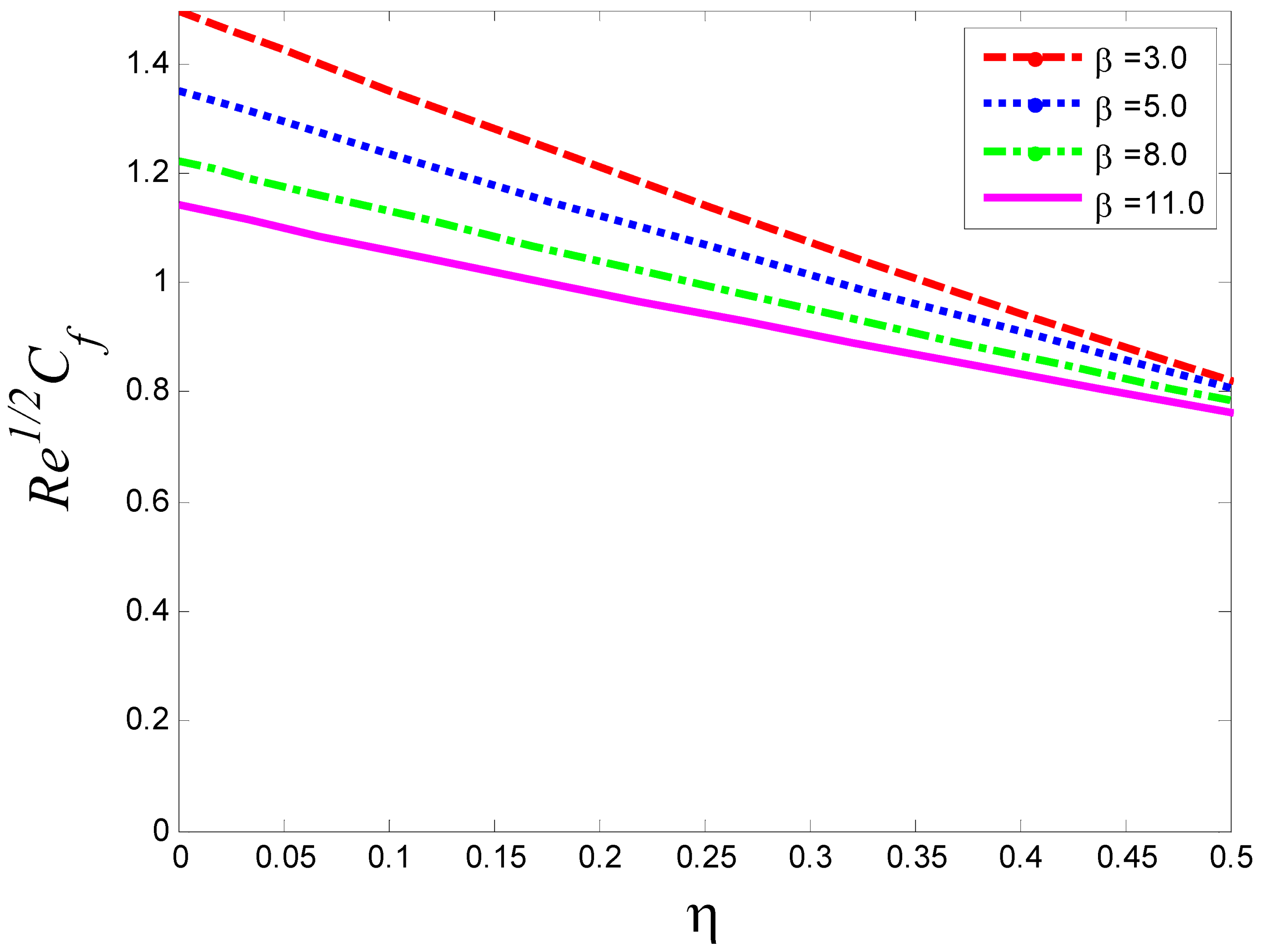
• It is concluded that the skin friction coefficient increases with increasing values of $K^{*}$ and $Fr$, but the opposite trend is seen for increasing magnitudes of $\beta$.
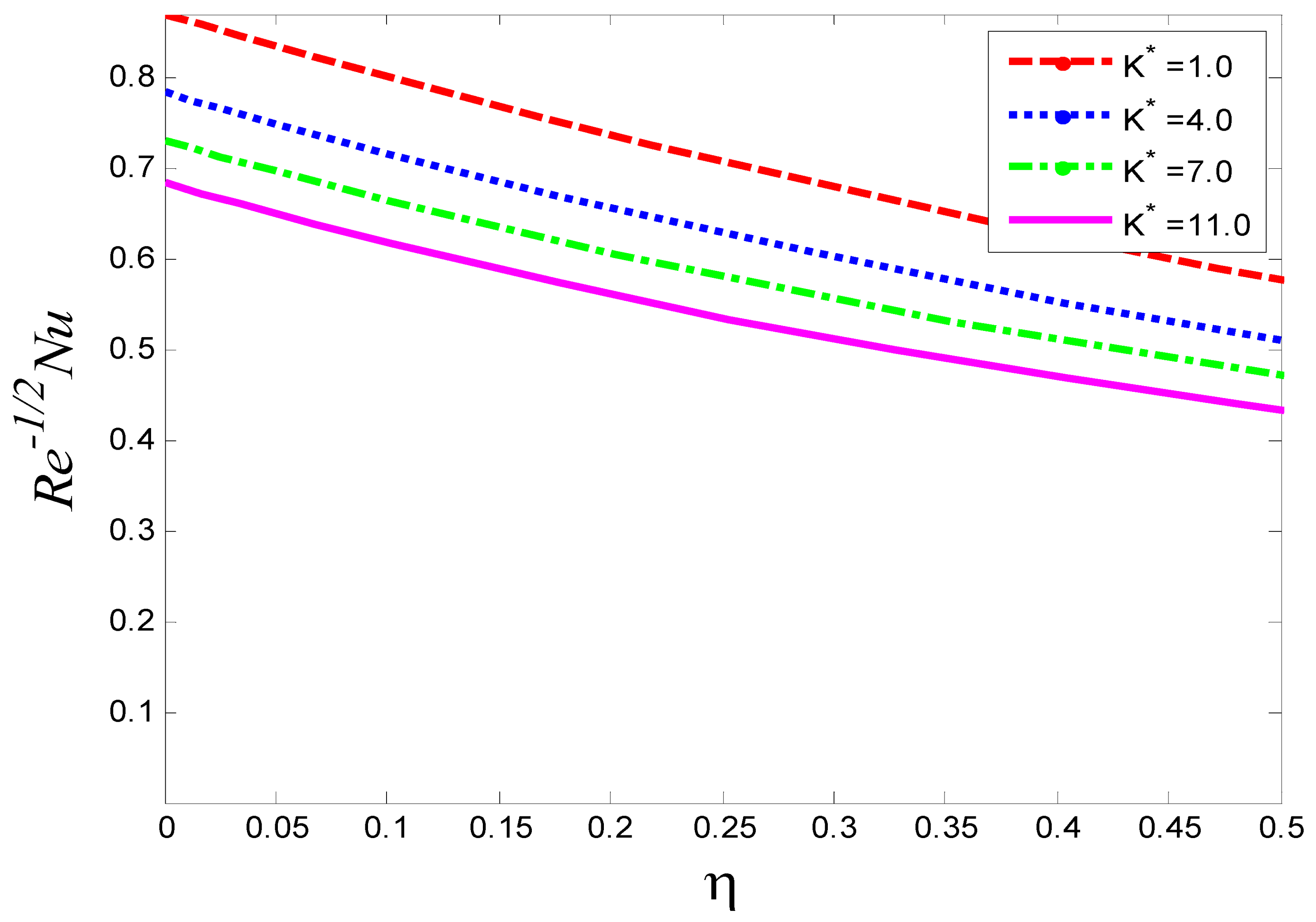
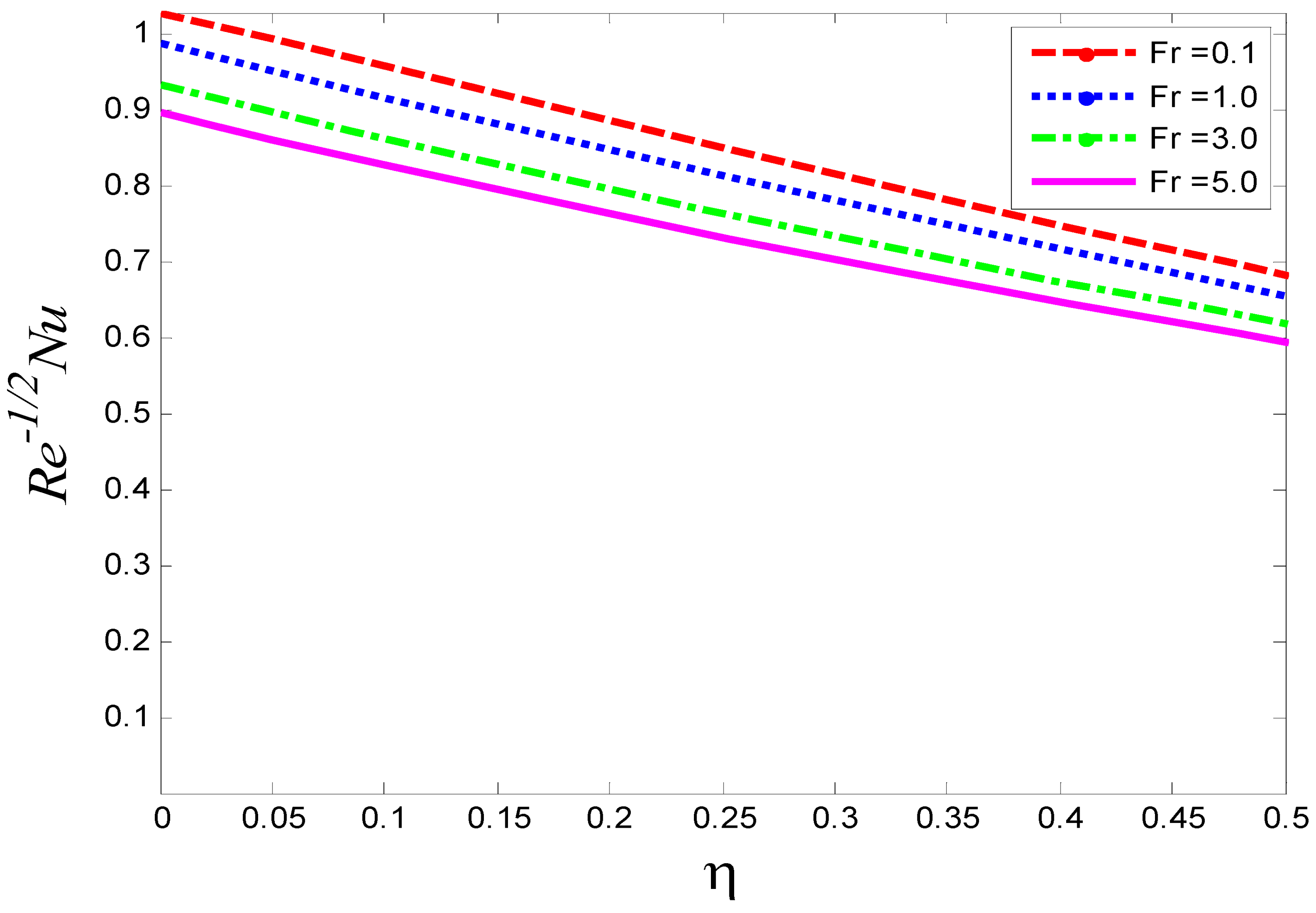
• The Nusselt number is elevated against elevating values of $\beta$ and the opposite action is viewed for increasing $K^{*}$ and $Fr$.
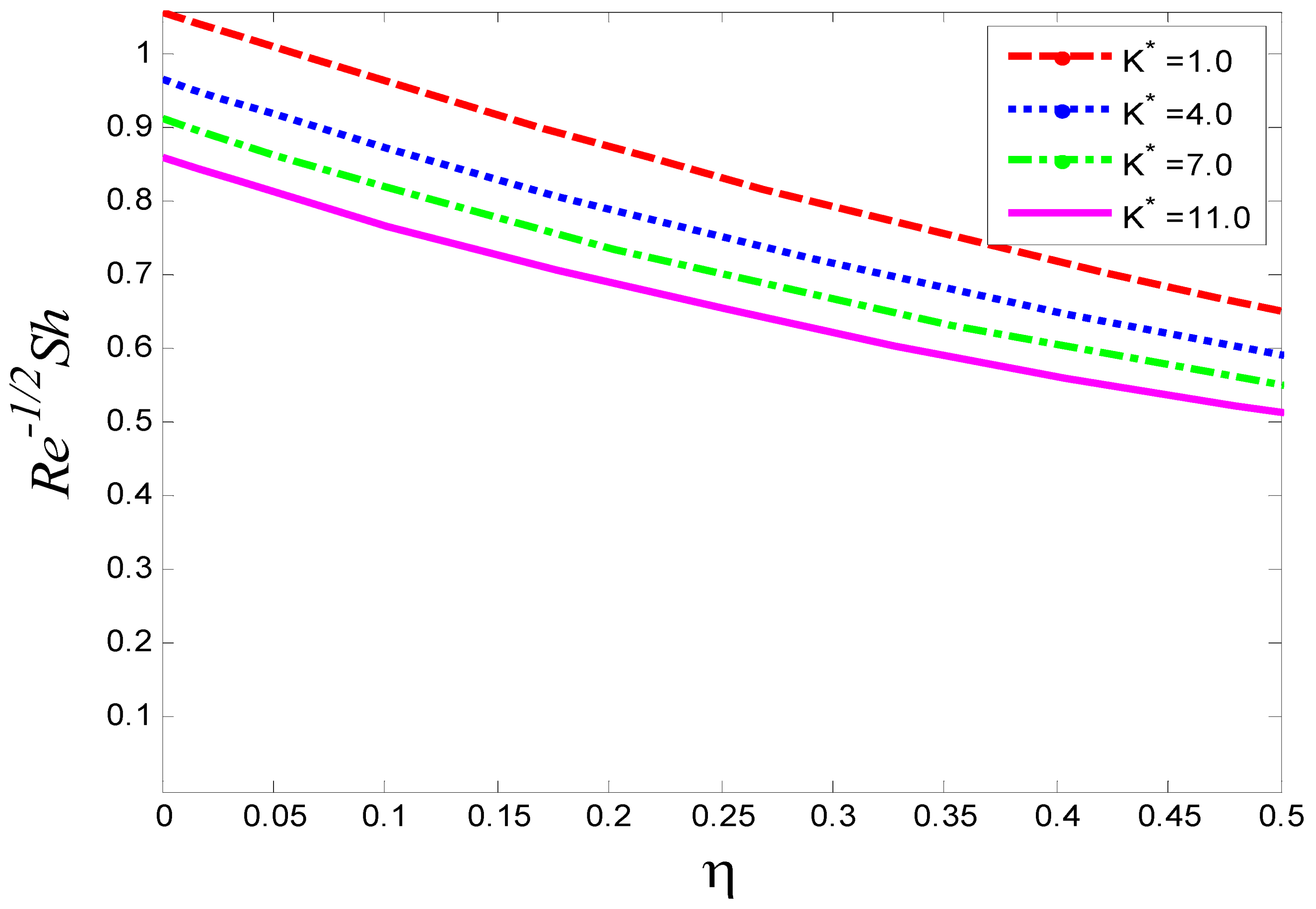
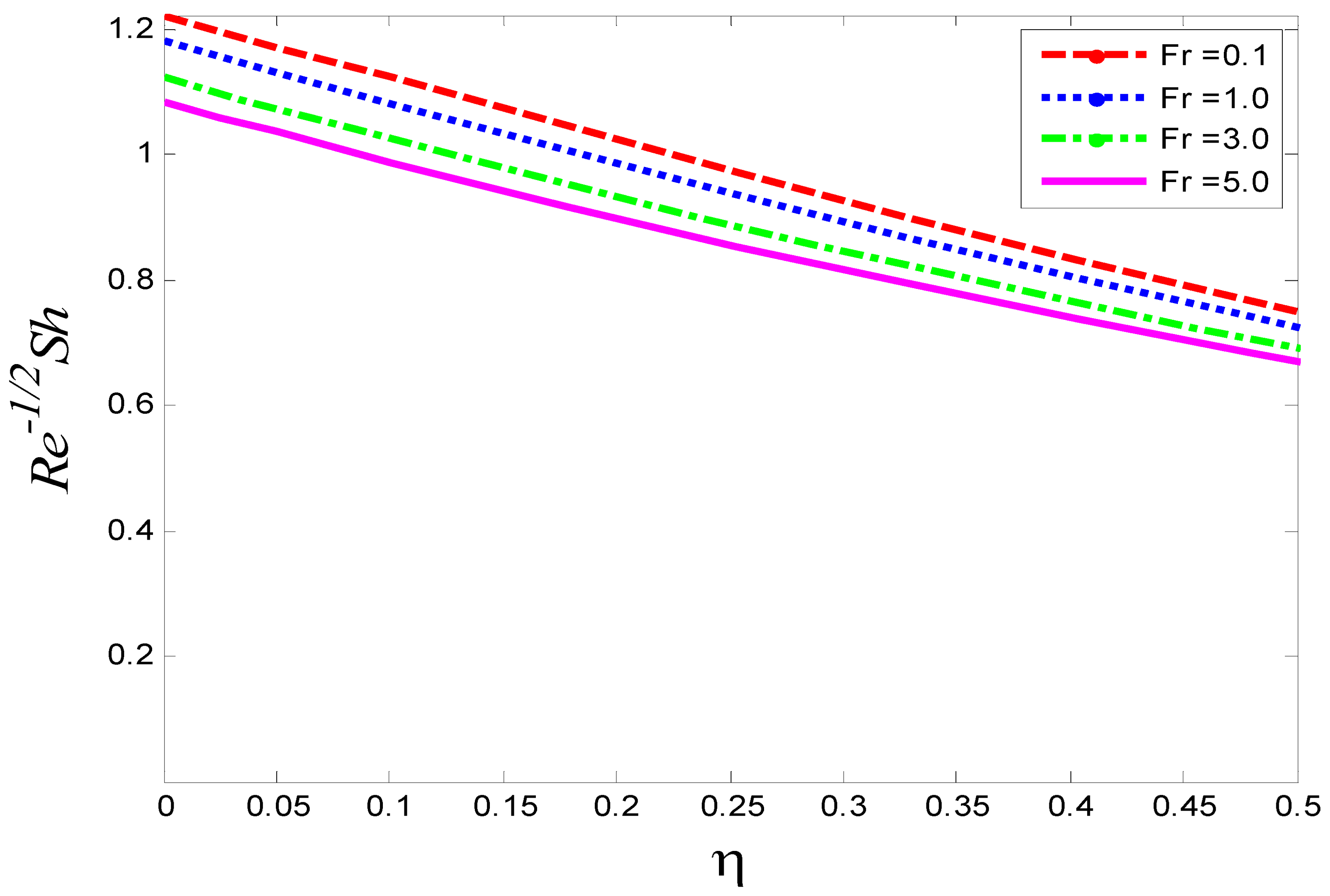
• The Sherwood number fleshes out an increasing attitude for increasing $\beta$ and shows the decreasing trend for augmenting $K^{*}$ and $Fr$.
• The present results for such a special case are compared with the previously published results and there is nice agreement between them, which validates the accuracy of the current results.
• In the future, this model can be extended to nanofluid and hybrid nanofluid with different fluid characteristics.
• This can also be extended to analyze the impact of reduced gravity on this model.

References

- Sahoo, B.; Do, Y. Effects of slip on sheet-driven flow and heat transfer of a third grade fluid past a stretching sheet. Int. Commun. Heat Mass Transf. 2010, 37, 1064–1071. [Google Scholar] [CrossRef]
- Sahoo, B. Flow and heat transfer of a non-Newtonian fluid past a stretching sheet with partial slip. Commun. Nonlinear Sci. Numer. Simul. 2010, 15, 602–615. [Google Scholar] [CrossRef]
- Sahoo, B. Hiemenz flow and heat transfer of a non-Newtonian fluid. Commun. Nonlinear Sci. Numer. Simul. 2009, 14, 811–826. [Google Scholar] [CrossRef]
- Pakdemirli, M. The boundary layer equations of third-grade fluids. Int. J. Non-Linear Mech. 1992, 27, 785–793. [Google Scholar] [CrossRef]
- Sahoo, B.; Sharma, H.G. MHD flow and heat transfer from continuous surface in uniform free stream of non-Newtonian fluid. Appl. Math. Mech. 2007, 28, 1467–1477. [Google Scholar] [CrossRef]
- Javanmard, M.; Taheri, M.H.; Ebrahimi, S.M. Heat transfer of third-grade fluid flow in a pipe under an externally applied magnetic field with convection on wall. Appl. Rheol. 2008, 28. [Google Scholar] [CrossRef]
- Hayat, T.; Khan, M.I.; Waqas, M.; Alsaedi, A.; Yasmeen, T. Diffusion of chemically re-active species in third grade fluid flow over an exponentially stretching sheet considering magnetic field effects. Chin. J. Chem. Eng. 2017, 25, 257–263. [Google Scholar] [CrossRef]
- Sahoo, B.; Poncet, S. Flow and heat transfer of a third grade fluid past an exponentially stretching sheet with partial slip boundary condition. Int. J. Heat Mass Transf. 2011, 54, 5010–5019. [Google Scholar] [CrossRef] [Green Version]
- Madhu, M.; Shashikumar, N.S.; Gireesha, B.J.; Kishan, N. Second law analysis of MHD third-grade fluid flow through the microchannel. Pramana 2021, 95, 4. [Google Scholar] [CrossRef]
- Zhang, L.; Bhatti, M.M.; Michaelides, E.E. Electro-magnetohydrodynamic flow and heat transfer of a third-grade fluid using a Darcy-Brinkman-Forchheimer model. Int. J. Numer. Methods Heat Fluid Flow 2020, 31, 2623–2639. [Google Scholar] [CrossRef]
- Shehzad, S.A.; Abbasi, F.M.; Hayat, T.; Ahmad, B. Cattaneo-Christov heat flux model for third-grade fluid flow towards exponentially stretching sheet. Appl. Math. Mech. 2016, 37, 761–768. [Google Scholar] [CrossRef]
- Reddy, G.J.; Hiremath, A.; Kumar, M. Computational modeling of unsteady third-grade fluid flow over a vertical cylinder: A study of heat transfer visualization. Results Phys. 2018, 8, 671–682. [Google Scholar] [CrossRef]
- Chu, Y.M.; Khan, M.I.; Khan, N.B.; Kadry, S.; Khan, S.U.; Tlili, I.; Nayak, M.K. Significance of activation energy, bio-convection and magnetohydrodynamic in flow of third grade fluid (non-Newtonian) towards stretched surface: A Buongiorno model analysis. Int. Commun. Heat Mass Transf. 2020, 118, 104893. [Google Scholar] [CrossRef]
- Nadeem, S.; Saleem, S. Analytical study of third grade fluid over a rotating vertical cone in the presence of nanoparticles. Int. J. Heat Mass Transf. 2015, 85, 1041–1048. [Google Scholar] [CrossRef]
- Fosdick, R.L.; Rajagopal, K.R. Thermodynamics and stability of fluids of third grade. Proc. R. Soc. Lond. Ser. A Math. Phys. Sci. 1980, 369, 351–377. [Google Scholar] [CrossRef]
- Forchheimer, P. Wasserbewegung durch boden. Z. Ver. Deutsch Ing. 1901, 45, 1782–1788. [Google Scholar]
- Muskat, M.; Wyckoff, R.D. The flow of homogeneous fluids through porous media. Soil Sci. 1946, 46, 169. [Google Scholar] [CrossRef]
- Seddeek, M. Influence of viscous dissipation and thermophoresis on Darcy–Forchheimer mixed convection in a fluid saturated porous media. J. Colloid Interface Sci. 2006, 293, 137–142. [Google Scholar] [CrossRef] [PubMed]
- Pan, H.; Rui, H. Mixed element method for two-dimensional Darcy-Forchheimer model. J. Sci. Comput. 2012, 52, 563–587. [Google Scholar] [CrossRef]
- Ramzan, M.; Gul, H.; Zahri, M. Darcy-Forchheimer 3D Williamson nanofluid flow with generalized Fourier and Fick’s laws in a stratified medium. Bull. Pol. Acad. Sciences. Tech. Sci. 2020, 68, 327–335. [Google Scholar]
- Hayat, T.; Haider, F.; Muhammad, T.; Alsaedi, A. An optimal study for Darcy-Forchheimer flow with generalized Fourier’s and Fick’s laws. Results Phys. 2017, 7, 2878–2885. [Google Scholar] [CrossRef]
- Grillo, A.; Carfagnay, M.; Federicoz, S. The Darcy-Forchheimer law for modelling fluid flow in biological tissues. Theor. Appl. Mech. 2014, 41, 283–322. [Google Scholar] [CrossRef]
- Knabner, P.; Roberts, J.E. Mathematical analysis of a discrete fracture model coupling Darcy flow in the matrix with Darcy–Forchheimer flow in the fracture. ESAIM Math. Model. Numer. Anal. 2014, 48, 1451–1472. [Google Scholar] [CrossRef] [Green Version]
- Khan, M.; Salahuddin, T.; Malik, M.Y. Implementation of Darcy–Forchheimer effect on magnetohydrodynamic Carreau–Yasuda nanofluid flow: Application of Von Kármán. Can. J. Phys. 2019, 97, 670–677. [Google Scholar] [CrossRef]
- Nagaraja, B.; Gireesha, B.J.; Soumya, D.O.; Almeida, F. Characterization of MHD convective flow of Jeffrey nanofluid driven by a curved stretching surface by employing Darcy–Forchheimer law of porosity. Waves Random Complex Media 2022, 1–20. [Google Scholar] [CrossRef]
- Kumar, D.; Sinha, S.; Sharma, A.; Agrawal, P.; Dadheech, P.K. Numerical study of chemical reaction and heat transfer of MHD slip flow with Joule heating and Soret–Dufour effect over an exponentially stretching sheet. Heat Transf. 2021, 51, 1939–1963. [Google Scholar] [CrossRef]
- Ishak, A. MHD boundary layer flow due to an exponentially stretching sheet with radiation effect. Sains Malays. 2011, 40, 391–395. [Google Scholar]
- Sajid, M.; Hayat, T. Influence of thermal radiation on the boundary layer flow due to an exponentially stretching sheet. Int. Commun. Heat Mass Transf. 2008, 35, 347–356. [Google Scholar] [CrossRef]
- Nadeem, S.; Haq, R.U.; Khan, Z. Heat transfer analysis of water-based nanofluid over an exponentially stretching sheet. Alex. Eng. J. 2013, 53, 219–224. [Google Scholar] [CrossRef] [Green Version]
- Bidin, B.; Nazar, R. Numerical solution of the boundary layer flow over an exponentially stretching sheet with thermal radiation. Eur. J. Sci. Res. 2009, 33, 710–717. [Google Scholar]
- Magyari, E.; Keller, B. Heat and mass transfer in the boundary layers on an exponentially stretching continuous surface. J. Phys. D Appl. Phys. 1999, 32, 577. [Google Scholar] [CrossRef]