Self-Similarity in Magnetostrictive Materials: An Experimental Point of View

Abstract

Magnetostrictive behavior is characterized by a complex coupling between magnetic and mechanical quantities. While this behavior can be quite easily exploited for both actuation and sensing or energy conversion purposes, the complex hysteresis interaction between magnetization and magnetic field and mechanical stress and strain is hard to model. Nevertheless, magnetic and magnetostrictive experimental curves are quite self-similar, assuming stress as self-similarity parameter. The quantification of this concept would help modeling. Here, this concept is quantified and experimentally confirmed over different types of magnetostrictive samples.

1. Introduction

Magnetostrictive materials (MMs) are the ones showing the unique feature to couple mechanical quantities, as stress and strain, with magnetic ones, as magnetic field and induction [1]. This means that they can directly convert mechanical energy into electromagnetic one, or vice versa, and this can be done with higher efficiency with respect to conventional methods [2]. For these reasons, since early 2000s, they have experienced such a growing technological interest as to be proposed as key elements in innovative sensors and actuators, both for bulk and Micro Electro-Mechanical Systems (MEMS) devices [3]. On the other hand, their macroscopic behavior is rather complicated, and accurate modeling of magnetostrictive devices is still under development.

It is well known that the experimental magnetic characteristics of magnetostrictive materials show nonlinear behavior, hysteresis, and magnetic saturation. Furthermore, by increasing the compressive applied stress, the magnetic characteristics drop down. In particular, the magnetic permeability decreases and the curves approach saturation at higher magnetic field and the material is said to be magnetically harder. Similar behaviors are observed for magnetostrictive curves [1] and also for ferromagnetic materials [4,5]. These properties can be exploited for sensing [6,7] and for non-destructive testing [4].

Figure 1 shows typical characteristics of a magnetostrictive material, with the aforementioned behavior. It is noticeable that the M-H curves at constant applied stresses exhibit a similar shape. This leads to the conjecture that it is possible to rescale the input field by introducing a new state variable u as a function of the magnetic field and stress in such a way that, in terms of the new input u, all magnetization curves coincide. This phenomenon is called self-similarity. In literature, very few works have been published on this particular property, such as Reference [8,9] for magnetocaloric materials, and this confirms the novelty of the results reported in this manuscript.

The rest of the paper is organized as follows. In Section 2, the experimental setup to measure the magnetic curves and the relevant quantities and procedures are described. In Section 3, the self-similarity concept is discussed and verified over the most common magnetostrictive materials. The Conclusions section ends the paper.

2. Setup

In order to explore the self-similarity in MMs, their experimental characterization is of paramount importance. Then, in this section, we present the experimental setup developed and used to this purpose, while, in the next sections, the typical characteristics and behavior of some MMs are shown and discussed.

In an overall view, MMs can be studied as a 2 inputs—2 outputs system. In particular, the inputs are the mechanical stress $\sigma$ and magnetic field H, while the corresponding outputs are the strain$\epsilon$ and magnetization M. In Figure 2a, a simplified block diagram of the experimental setup is shown, while, in Figure 2b, a sketch of the setup used to characterize MMs is depicted. The core of Figure 2a is the light gray box representing the magnetostrictive material, where the blue solid arrows are the two inputs, while the red solid ones are the outputs. Note that M and B are related to each other through the simple Equation (3) below. Furthermore, the red dots and text box represent the measurements points and the devices, respectively.

The magnetic field is generated with two excitation coils (380-turns each one) located in the central column of a double C-shaped iron yokes (cross section: 30 mm × 30 mm), which behave as a magnetic circuit. The two excitation coils are supplied by a power amplifier (KEPCO BOP 50-20MG), and the latter is driven by an arbitrary waveform generator (Aim-TTi TGA12104), as reported in Figure 2a. The ferromagnetic central column is split into two parts: one (the bottom) is bound with the remaining iron magnetic circuit, while the second part (top) is connected to the Universal Testing Machine (UTM, Lloyd LRX Plus—5 kN), through Belleville springs and a load cell (AEP TS—2 kN), behaving both as a mechanical chain able to provide the stress to the magnetostrictive sample and a magnetic path. In particular, the springs are inserted in the mechanical chain with the aim to mitigate the direct magnetostrictive effect when a constant stress and a magnetic field are applied. Moreover, the top part of the column can slide in a square hole made in the upper horizontal arm of the iron circuit, then allowing both the stress transferring and the magnetic circuit closing.

The sample to be characterized has been placed between the two parts of the central column where the excitation coils are installed, and it is equipped with two strain gauges glued on opposite faces. The overall deformation is the computed average of the two measurement points; therefore, any non-uniform stress transfer to the material, due to superficial imperfections, is then compensated. Around each sample is wounded a pickup coil, while a Hall effect probe, connected to a Gaussmeter (Lakeshore 475DSP), is installed horizontally in contact with the sample, in order to measure the applied magnetic field [10,11]. Both the inputs and outputs are measured by the aforementioned sensors and acquired with a Data AcQuisition board (NI SCXI-1000 chassis, with SCXI-1520 for analog signals acquisition and SCXI-1521b for strain gauges measurements).

The strain, mechanical stress, and magnetic field are directly measured with the corresponding measurement devices, while the magnetization is measured indirectly.

In particular, by defining S as the cross section of the sample, and N as the pickup coil turns number, through Faraday-Neumann-Lenz’s law of induction, it is possible to express the measured pickup coil voltage v (so, the electromotive force) as:

$$v=-\frac{\mathrm{d}{\Phi }}{\mathrm{d}t}=-NS\frac{\mathrm{d}B}{\mathrm{d}t},$$

(1)

where ${\Phi }$ is the linked magnetic flux, and B the magnetic induction. As a consequence, it is possible to obtain B as follows:

$$B=-\frac{1}{NS}{\int }_{t}v\mathrm{d}t.$$

(2)

Through a MATLAB^® code, the integration in Equation (2) is numerically executed in post-processing, in order to obtain the magnetic induction. Finally, the magnetization M can be computed from the relation:

$$B={\mu }_0(H+M)⟹M=\frac{B}{{\mu }_0}-H.$$

(3)

It is worth highlighting that, even if, from a mathematical point of view, the above written equations should be expressed in the vectorial form, the experimental setup and the measurement apparatus allow for having all the involved quantities directed along the principal axis. Then, all the quantities can be treated as scalars.

It is worth noting that the adopted UTM is strain velocity controlled. The different force values are applied to the material by a feedback control on the force sensor measurement and a null cross-head speed. The direct magnetostrictive effect, when a magnetic field is applied, counteracts the stress applied by the UTM, by increasing the latter because the cross-head speed control is not sufficient to compensate this variation of force in a short time. Consequently, some Belleville springs are introduced in the mechanical chain in order to have a more stable constant applied stress.

Finally, the characterization of a magnetostrictive sample consists of the measurement of the aforementioned outputs when one input changes and the other is constant. In other words, four different types of plots are achievable: M-H and $\epsilon$-H curves at different constant values of $\sigma$, and $\Delta B$-$\sigma$ (or B-$\sigma$) and $\epsilon$-$\sigma$ curves at different constant values of H. However, for the purposes of this manuscript, only the M-H curves at different stresses are needed and then shown.

3. Discussion

3.1. Self-Similarity Definition

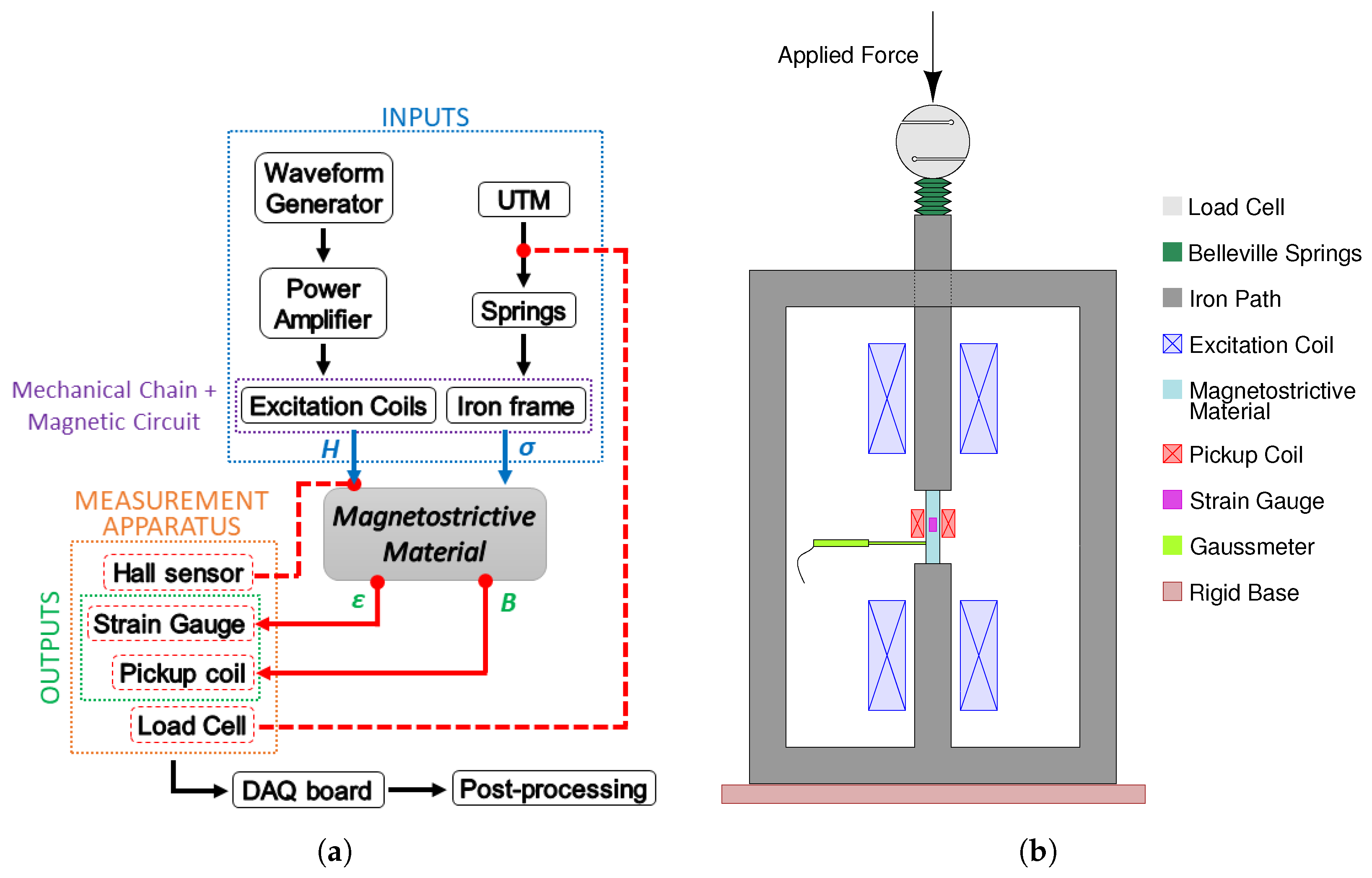
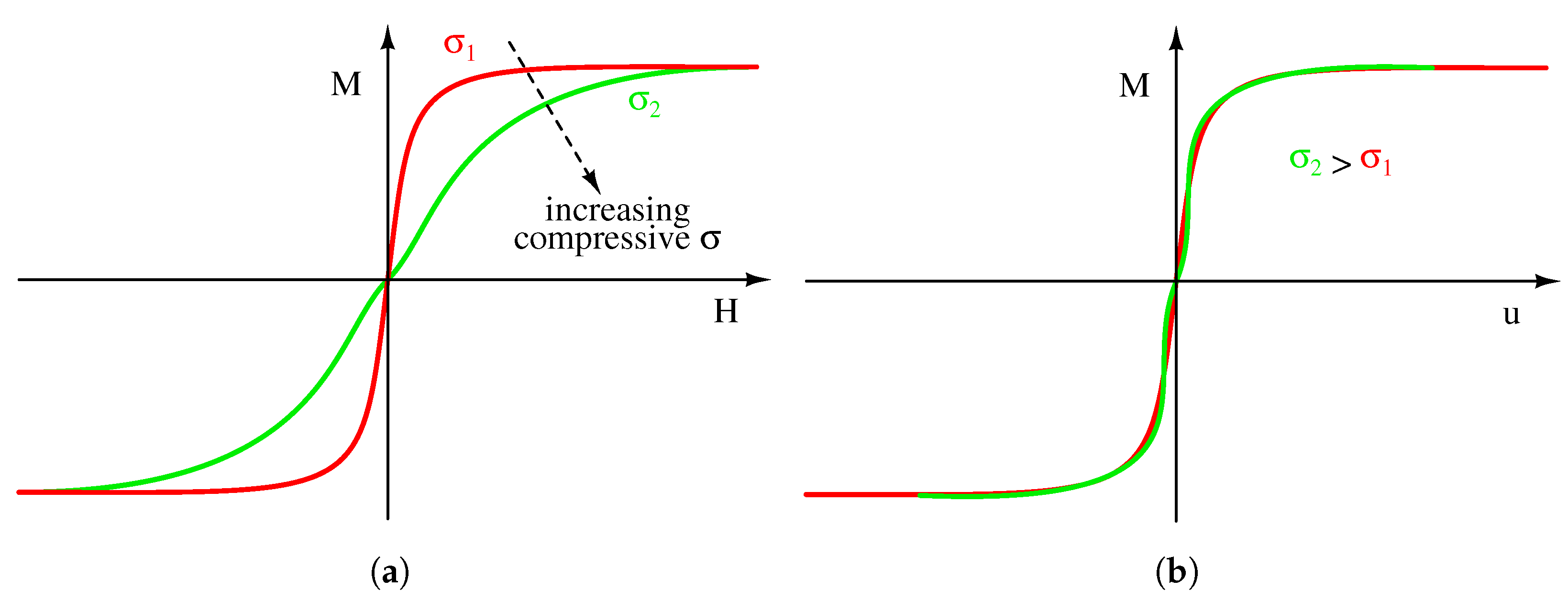
Figure 3a shows the typical qualitative magnetization characteristics of a NSA Galfenol sample at different stresses (hysteresis is neglected). There and in the following, it is assumed that all the involved physical quantities are aligned and uniform (e.g., the magnetostrictive sample has a regular and constant cross sectional area S, with stress $\sigma =F/S$, where F is the applied force, and the magnetic field H is directed along its longitudinal axis). Those curves can be represented as two general implicit relationships:

$${{\Psi }}_i(H,M,\epsilon ,\sigma )=0,i=1,2.$$

(4)

Indeed, from the practical point of view, it would be more convenient to solve explicitly the implicit Equations (4) with respect to $\epsilon$ and M and write them in the form:

$$\left\{\begin{array}{cc}\hfill \epsilon & =\epsilon (H,\sigma )\hfill \\ \hfill M& =M(H,\sigma )\hfill \end{array},\right.$$

(5)

which clearly distinguishes between the input and output quantities.

It can be observed that the M-H curves at different constant applied stresses ($\sigma$) have similar shapes, and the stress appears as a scaling parameter. Therefore, it is possible to introduce a new state variable $u=u(H,\sigma )$ that is function of the magnetic field and stress, in such a way that all M-u curves overlap, and reformulate Equations (5) as:

$$\left\{\begin{array}{cc}\hfill \epsilon & =\tilde{\epsilon }\left(u\right)\hfill \\ \hfill M& =\tilde{M}\left(u\right)\hfill \end{array},\right.$$

(6)

as shown in the illustration of Figure 3b. This behavior would be an experimental evidence of the self-similarity property of magnetostrictive materials, with u as self-similar variable. It is worth pointing out that the variable u, as shown in the following, appears to be substantial in modeling magnetostriction. Indeed, a suitable choice of u allows for building up an analytical phenomenological description of the most common magnetostrictive behavior, as reported in Reference [12]. Moreover, in this paper, we show this particular viewpoint of the self-similarity property, based on the experimental measurements, similar to what was done in Reference [8,9] for magnetocaloric materials with ferro-to-paramagnetic phase transitions.

One of the questions that this paper deals with is: can self-similarity be formally quantified for the most common magnetostrictive materials? This would be very beneficial for the mathematical modeling of the materials. Let us note that this approach has already been considered in modeling, even though not fully explicited and exploited. For example, in Reference [13,14], thermodynamic constraints led to the following expression for u:

$$u=\frac{H}{f\left(\sigma \right)},$$

(7)

where the function $f\left(\sigma \right)$ described the influence of different applied stresses on the magnetic characteristics of magnetostrictives.

In view of the mathematical modeling, the variable u defined as in Equation (7) may not be able to fully mimic the experimental magnetic and magnetostrictive behaviors of MMs at a very low magnetic field (near-zero H), as the ones reported in Reference [15,16,17]. It is, therefore, appropriate to modify the simple definition of u of Equation (7) in the form:

$$u=u(H,\sigma ,M)=\frac{H+b\left(\sigma \right)·m\left(M\right)}{f\left(\sigma \right)},$$

(8)

where the term $b\left(\sigma \right)·m\left(M\right)$ represents the feedback, the influence of which may become dominant at very low magnetic fields. Moreover, as suggested in Reference [18,19,20], the term $H+b\left(\sigma \right)·m\left(M\right)$ can be seen as the effective magnetic field, $H_e$. The formulation of u as reported in Equation (8) helps to take into account, in the modeling of MMs, the experimental behavior at a very low field, such as the residual magnetization and the inverse magnetostriction effect (Villari effect) at no field applied, i.e., $H=0$. Finally, it is worth noting that Equation (8) inserted in Equations (6) would be a simplified expression of Equation (4). Nevertheless, if $b\left(\sigma \right)$ is sufficiently small, $f\left(\sigma \right)$ is sufficiently large, and $m\left(M\right)$ is a continuously differentiable function, then the relations reported in Equations (6) and (8) implicitly define a constitutive law $M=M(H,\sigma )$. The problem of analytical representation of the function $M(H,\sigma )$ is generally difficult. We propose to use the self-similar character of the experimental curves and reduce the complexity of the problem by representing the constitutive function $M(H,\sigma )$ of two variables by means of four functions of one variable: $M\left(u\right)$, $f\left(\sigma \right)$, $b\left(\sigma \right)$, and $m\left(M\right)$.

Once the expression of u has been considered, the three functions, $b\left(\sigma \right)$, $m\left(M\right)$, and $f\left(\sigma \right)$, must be identified. The most simple and robust method to identify if and how much two or more different continuous curves are similar among them is to compute the difference of the areas under the curves, with respect to the abscissa u. The smaller this difference, the stronger the similarity. In the case of magnetic characteristics, because of the odd symmetry, this property can be checked by considering only the first quadrant and can be written as:

$$\min |A_{{\sigma }_{min}}-A_{{\sigma }_{max}}|,$$

(9)

where $A_{{\sigma }_{min}}$ is the area under the M-u curve at the minimum applied stress, i.e.,

$$A_{{\sigma }_{min}}={\int }_0^u{M}_{{\sigma }_{min}}\mathrm{d}u,$$

(10)

while $A_{{\sigma }_{max}}$ is the area under of the M-u curve at the maximum applied stress, i.e.

$$A_{{\sigma }_{max}}={\int }_0^u{M}_{{\sigma }_{max}}\mathrm{d}u.$$

(11)

This minimization is computed with respect to the parameters of the functions $b\left(\sigma \right)$, $m\left(M\right)$, and $f\left(\sigma \right)$. Once the minimum of Equation (9) is obtained, the output parameters are available to be used in modeling of MMs.

It is noticeable that it could be possible to use the $\epsilon$-H curve also, i.e., the first of Equation (6), in order to test the self-similar character. Nevertheless, it is proven in the literature that both magnetic and magnetostrictive characteristics are analytically correlated by the principles of thermodynamics [14,21], and, then, out of experimental errors, the self-similarity concept applies to both at the same extent. However, contrary to the magnetic curves, the magnetostrictive ones would need a much higher magnetic field to reach saturation [3,22], and, nevertheless, magnetostrictive curves show different saturation values, with respect to the applied stress. Thus, magnetic curves were preferred in this experimental analysis, and the verification of the correlation is left to future works.

The choice of the functions $b\left(\sigma \right)$, $m\left(M\right)$, and $f\left(\sigma \right)$ is indeed different for different materials. In this manuscript, we considered three different MMs: two twin samples of Galfenol, wherein one is non-stress annealed, and the other is stress-annealed; and a sample of Terfenol-D. The samples were manufactured by the company $Td$Vib, LLC (Boone, IA, USA); see Reference [23].

3.2. NSA Galfenol

Galfenol is an Iron-Gallium alloy (Fe${}_{81.6}$Ga${}_{18.4}$), and it is textured polycrystalline, grown with free-standing zone melt (FSZM) technique by $Td$Vib. It has good magnetic, mechanical, and magnetostrictive properties. In particular, it does not show very large magnetostriction values (about 200–250 ppm) in comparison with other MMs but has better magnetic characteristics (about 1.8–2 T magnetic saturation) than Terfenol-D (about 0.9–1 T magnetic saturation; see Section 3.4 for further details). As a consequence, it is particularly suitable for sensing and energy harvesting use [22]. The Galfenol samples adopted for the experimental measurements are both 30 mm long with a diameter of 5 mm.

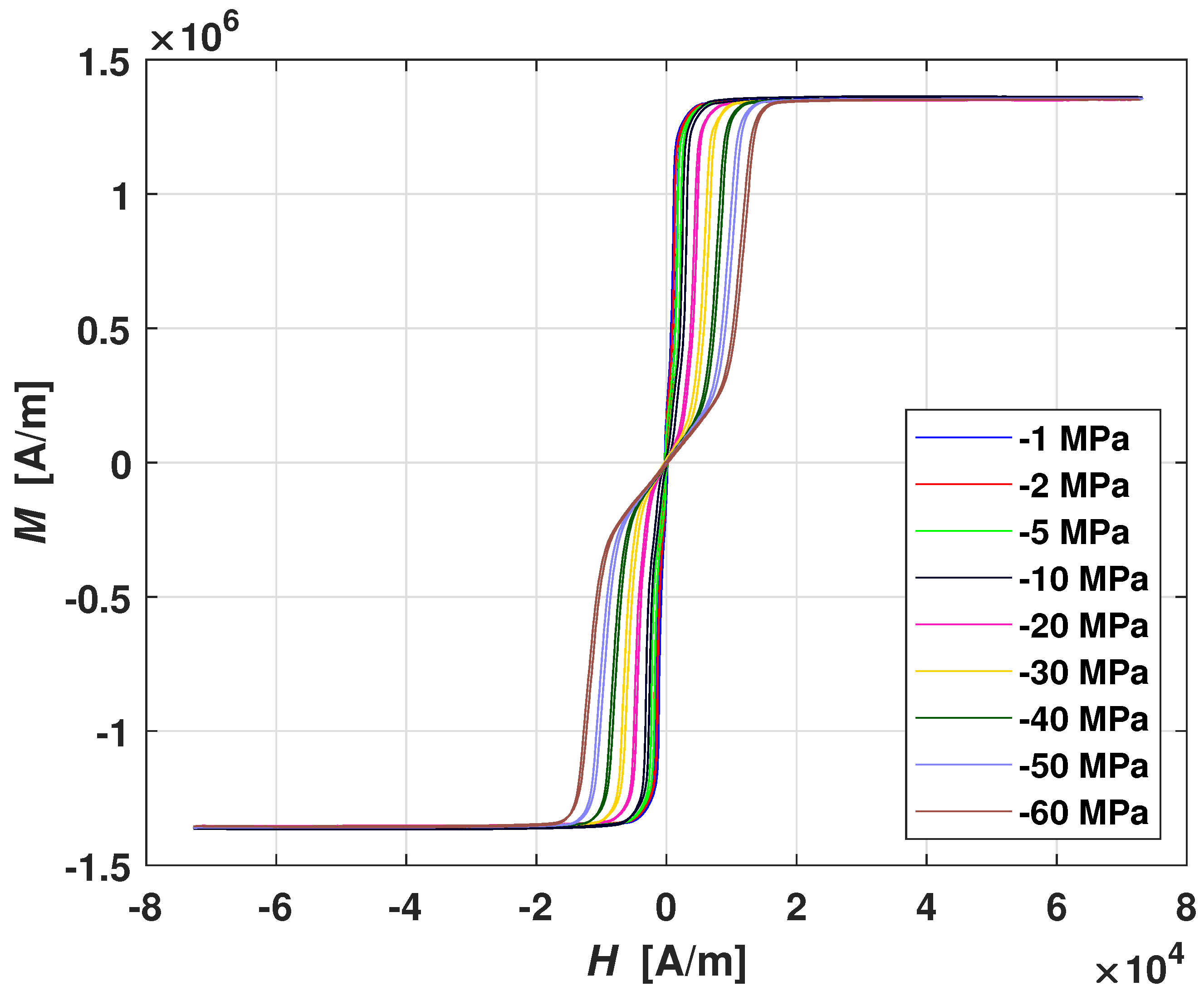
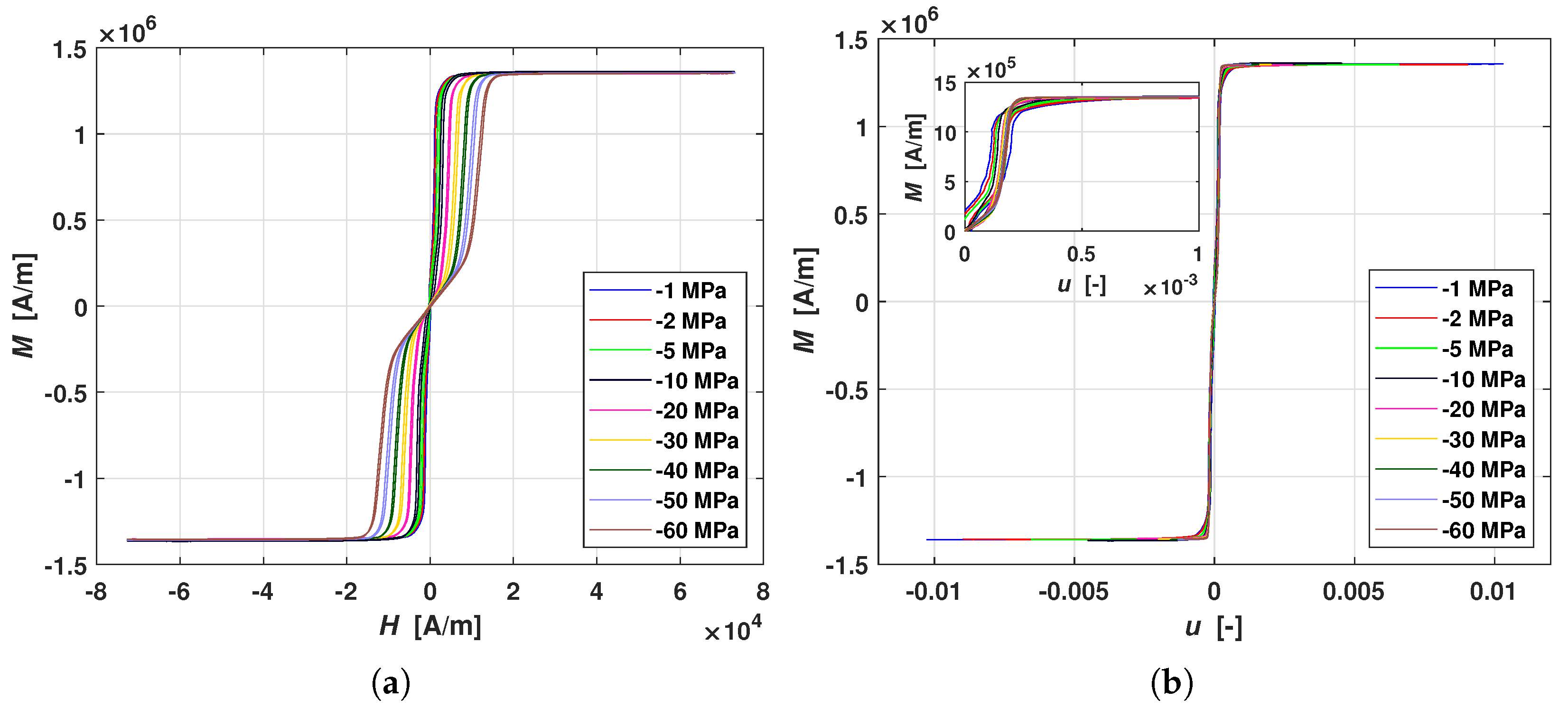
The magnetic characteristics of NSA Galfenol at different constant applied stresses are shown in Figure 4a. It is possible to note a very narrow hysteresis loop, low coercive field, low saturation field, and high saturation magnetization. Moreover, it is noticeable that, by increasing the compressive stress, the initial magnetic permeability decreases. These experimental data suggest to use a simple definition of the feedback term and $f\left(\sigma \right)$, reported in Equation (8). In particular, $b\left(\sigma \right)$ is a constant parameter $\beta$, and $m\left(M\right)$ is the magnetization itself, while $f\left(\sigma \right)=\gamma (\sigma +{\sigma }_0)$ is a linear function of the applied $\sigma$, i.e.,

$$u=\frac{H+\beta ·M}{\gamma (\sigma +{\sigma }_0)}=\frac{H+\beta ·M}{-(\sigma +{\sigma }_0)},$$

(12)

where $\gamma$ has a mere meaning of a dimensional scaling factor, and, in this case, because compressive stress has been defined as negative, it is equal to −1, while ${\sigma }_0$ is another constant parameter. The self-similarity problem can be computed by solving the Equation (9) with respect to $\beta$ and ${\sigma }_0$ parameters.

The whole problem is described as follows:

$$\begin{array}{cc}\hfill \underset{\beta ,{\sigma }_0}{\min }& |A_{{\sigma }_{min}}-A_{{\sigma }_{max}}|,\hfill \end{array}$$

(13)

$$\begin{array}{cc}\hfill A_{{\sigma }_{min}}& ={\int }_0^u{M}_{{\sigma }_{min}}\mathrm{d}u,\hfill \end{array}$$

(14)

$$\begin{array}{cc}\hfill A_{{\sigma }_{max}}& ={\int }_0^u{M}_{{\sigma }_{max}}\mathrm{d}u,\hfill \end{array}$$

(15)

$$\begin{array}{cc}\hfill u& =\frac{H+\beta ·M}{-(\sigma +{\sigma }_0)}.\hfill \end{array}$$

(16)

From the computational point of view, the minimization problem in the set of Equations (13)–(16) has been performed by considering only the average curve of each hysteresis loop of the experimental data shown in Figure 4a. Moreover, in principle, the minimization problem could be extended to all the experimental data, i.e., all the mechanical stress-range curves. However, this is not necessary because, by minimizing the area between the M-u curves at minimum and maximum stress, the areas computed for the other stress are just included, due to intrinsic magnetostrictive behaviors.

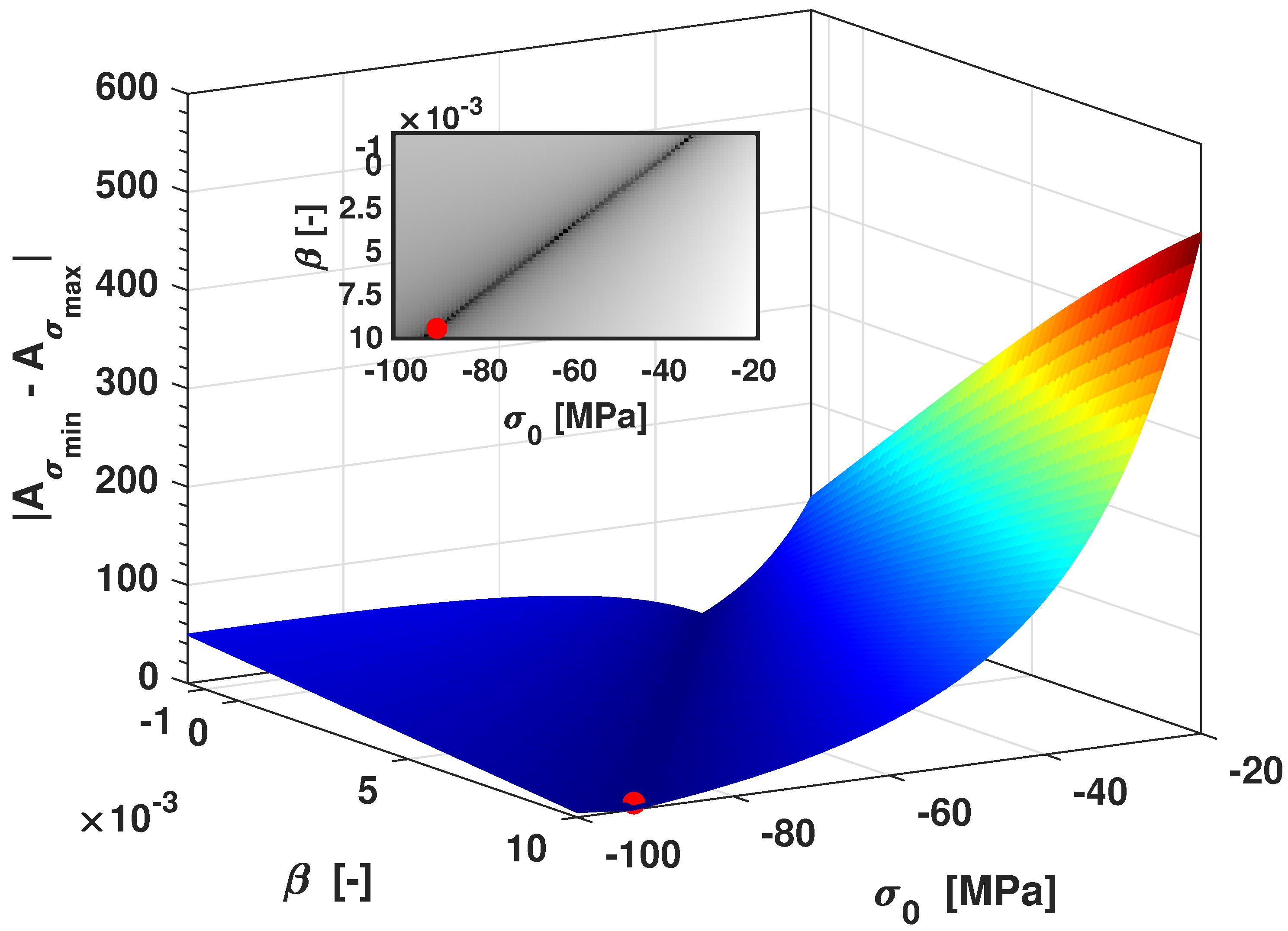
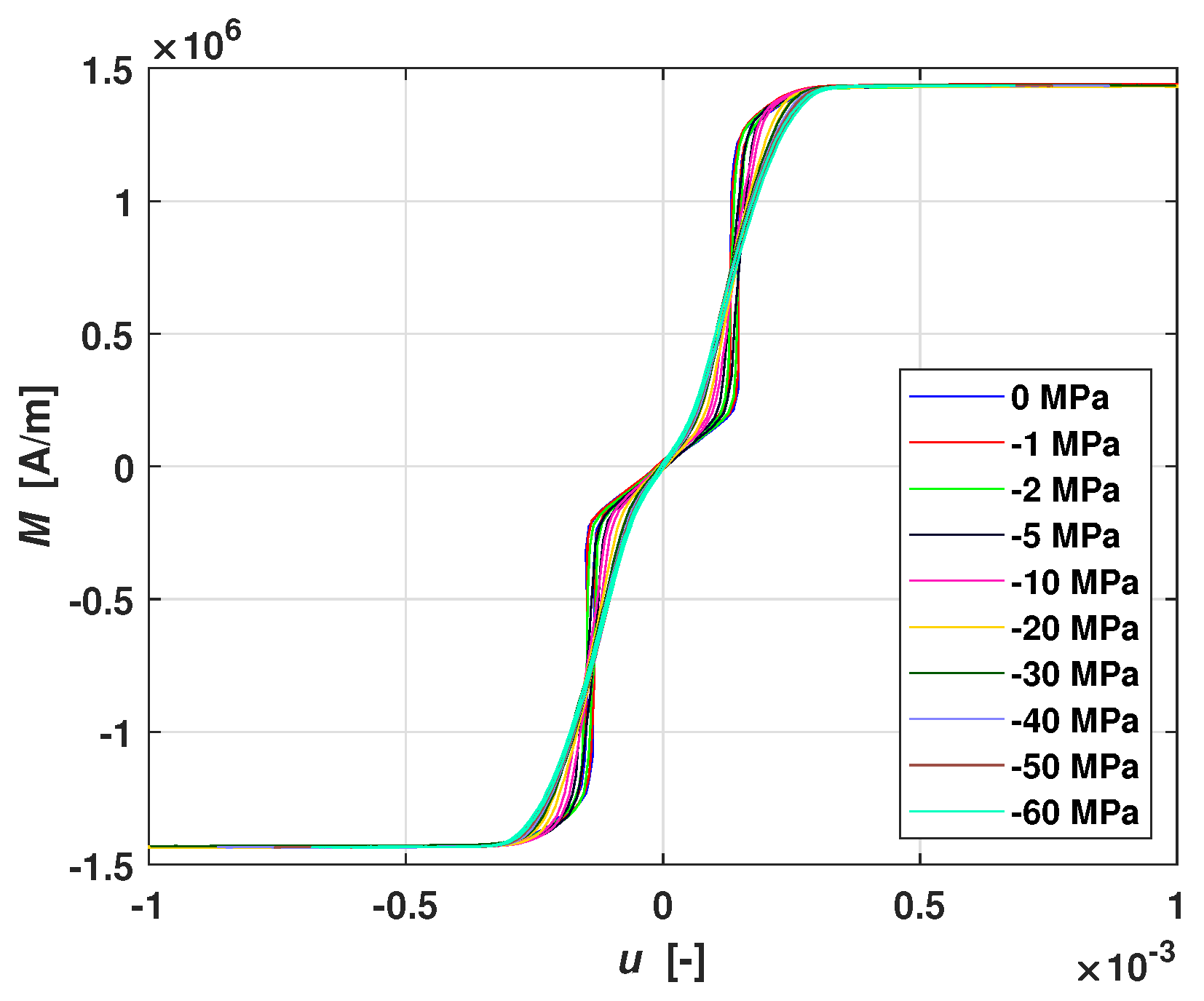
In Figure 5, the minimization problem as reported in the set of Equations (13)–(16) for NSA Galfenol is shown. The minimum of the areas difference is obtained for $\beta =-3.03\times {10}^{-4}$ and ${\sigma }_0=-6$ MPa. Figure 4b shows the M-u curves at different applied stresses, where u has been computed according to Equation (16) with the aforementioned $\beta$ and ${\sigma }_0$ parameters values. Note that all the curves almost overlap, which confirms that Equation (12) describes self-similarity in an appropriate way. Furthermore, in Figure 5, we see a zone, as in the dark gray river bed of the inset, where $|A_{{\sigma }_{min}}-A_{{\sigma }_{max}}|$ is very small. This means that it would be an almost linear combination of $\beta$ and ${\sigma }_0$ that minimizes the difference of the areas, and where the self-similarity is observable. However, the red dot shows the minimum of the surface in the considered range of values.

3.3. SA Galfenol

SA Galfenol differs from NSA ones because a built-in stress has been “frozen” into the material, during a post-manufacturing process. The built-in stress value is not provided with the sample characteristics. However, it essentially consists of a combination of magnetic field, high temperature, and mechanical stress applied to the material, for some time. Following that, a built-in stress remains in the magnetostrictive sample, which generates an uniaxial anisotropy that avoids the need for an external pre-stress mechanism [24,25]. This is visible in Figure 6a, where SA Galfenol magnetic characteristics at different applied stresses are shown. It is observable that, in this case, all the curves show the same initial magnetic permeability (linear behavior at low H), which is similar to the ones shown in Figure 4a at high compressive stress. Indeed, the built-in stress acts in the material as an external applied pre-stress.

The minimization problem for SA Galfenol is exactly the same of NSA ones, i.e., the set of Equations (13)–(16). Figure 7 shows the minimization results for SA Galfenol. In particular, the red dot indicates the minimum of the area difference that is obtained at $\beta =9.6\times {10}^{-3}$ and ${\sigma }_0=-91$ MPa. In Figure 6b, we represent the M-u curves at different applied stresses, where u has been computed according to Equation (16) with the aforementioned $\beta$ and ${\sigma }_0$ parameter values. We see that all the curves almost overlap, so that they be quite accurately interpreted as a single curve. As for NSA Galfenol, also in Figure 7, we see a zone (dark gray) where $|A_{{\sigma }_{min}}-A_{{\sigma }_{max}}|$ is very small. This means that it is an almost linear combination of $\beta$ and ${\sigma }_0$ that minimizes the difference of the areas.

As reported previously, the term $\beta ·M$ (in the numerator in Equation (12)) represents the magnetic feedback and can be identified as an effective field $H_e$. Moreover, it is worth noting that, from a numerical point of view, the parameter $\beta$ can have any positive or slightly negative values. Indeed, for large negative values, the curves would be S-shaped crossing the second quadrant of the graph, so that M cannot be represented by a function of u any longer. On the other hand, from a physical point of view, small negative values of $\beta$ can be interpreted as a demagnetizing factor. Finally, the term ${\sigma }_0$ is dimensionally compatible with a constant pre-stress, and then, physically, it could be seen as a stress “frozen” in the material due to its annealing post-manufacturing process. As expected, this value for NSA Galfenol has been found to be low. On the other hand, for SA Galfenol, this value has been found to be quite high. This is due to the fact the the surface in Figure 7 shows different local minima (blue/green “river bed”) because an almost linear combination of $\beta$ and ${\sigma }_0$ minimizes the areas difference. These minima correspond to positive values of $\beta$, while, if we allow $\beta$ to be negative, then, the values of ${\sigma }_0$ are between −34 and −41 MPa.

These values of the pre-stress are compatible with “built-in stress” values reported in Reference [26]. For the sake of clarity, Figure 8 shows the self-similar curves M-u for SA Galfenol with minima of the areas difference found in the negative range of $\beta$ and for its corresponding ${\sigma }_0$. It is noticeable that a certain similarity is still visible.

3.4. Terfenol-D

Terfenol-D is a Terbium, Dysprosium, and Iron alloy, and its chemical composition is Tb${}_x$Dy${}_{1-x}$Fe${}_y$, where the commonly adopted concentrations are $0.27<x<0.3$ and $y<2$ [27]. It produces the largest elongation at room temperature among all MMs for a relatively low H. In particular, it exhibits a maximum strain of about 1000–1500 ppm at room temperature and magnetic saturation of about 1 T [28]. This makes Terfenol-D particularly suitable for micro-positioning and actuating purposes. In addition, it is often used as active element in energy harvesting device [29]. The sample used in our experimental measurements is 20 mm long with a square section of 25 mm${}^2$.

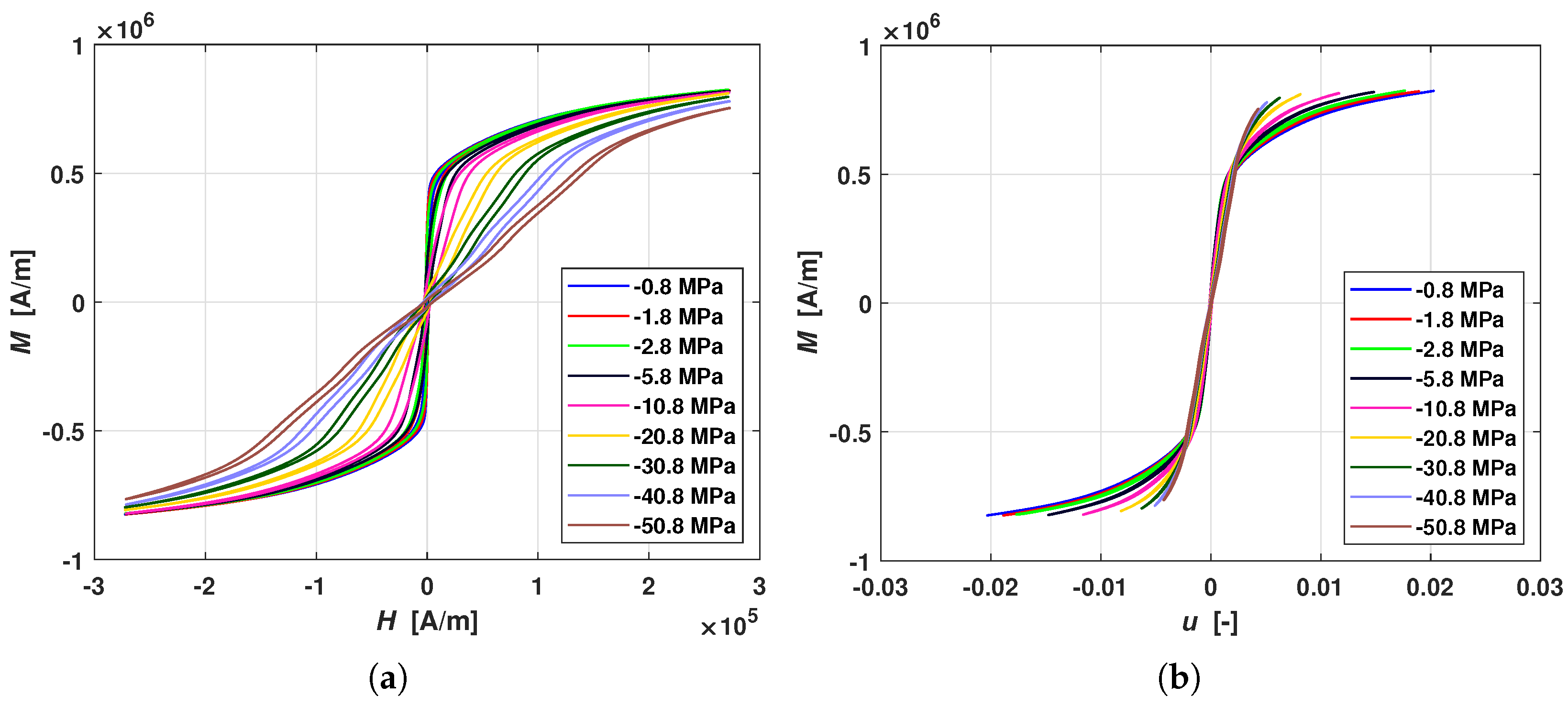
In Figure 9a, the magnetic characteristics for Terfenol-D at different applied constant stresses are reported. It is noticeable that saturation is reached at higher magnetic fields with respect to Galfenol. Indeed, the considered material is magnetically harder than Galfenol with stronger hysteresis effects. Moreover, the magnetic permeability decreases when the applied stress increases and exhibits a self-similar behavior typical also for Iron-Gallium alloys.

The overall minimization problem can be assumed as follows:

$$\begin{array}{cc}\hfill \underset{k,{\sigma }_0}{\min }& |A_{{\sigma }_{min}}-A_{{\sigma }_{max}}|,\hfill \end{array}$$

(17)

$$\begin{array}{cc}\hfill A_{{\sigma }_{min}}& ={\int }_0^u{M}_{{\sigma }_{min}}\mathrm{d}u,\hfill \end{array}$$

(18)

$$\begin{array}{cc}\hfill A_{{\sigma }_{max}}& ={\int }_0^u{M}_{{\sigma }_{max}}\mathrm{d}u,\hfill \end{array}$$

(19)

$$\begin{array}{cc}\hfill u=\frac{H+b\left(\sigma \right)·M}{\gamma (\sigma +{\sigma }_0)}& =\frac{H+\frac{k}{-(\sigma +{\sigma }_0)}·M}{-(\sigma +{\sigma }_0)},\hfill \end{array}$$

(20)

where, in this case, the function $b\left(\sigma \right)$ has been defined to be a hyperbolic function of $\sigma$ and the scaling parameter $\gamma$ still equal to −1. The choice of a nonlinear function $b\left(\sigma \right)$, instead of a constant parameter as for Galfenol, allows for identifying the feedback term more efficiently and obtaining a better fit with experimental data, by minimizing again the area difference.

Figure 10 illustrates the minimization problem for Terfenol-D. In particular, the red dot indicates the minimum of the area difference within the given range, which is reached for $k=5.1\times {10}^5$ and ${\sigma }_0=-14$ MPa. In Figure 9b, the M-u curves at different applied stresses are reported, where u has been computed as reported in Equation (20) with the aforementioned k and ${\sigma }_0$ parameters values. It is worth noting that the curves almost overlap near the origin with a linear-like behavior, while they slightly deviate in the knee area approaching the saturation. This is also related to the fact that, in experiments, it is difficult to reach complete saturation, and a part of the information necessary for the minimization procedure is missing. With the aim to improve the minimization algorithm, the average curve of the Terfenol hysteresis loops has been extrapolated according to the Law of Approach to Saturation (LAS), reported in Reference [30], up to 1000 kA/m. Still, due to the lack of experimental information about the large field asymptotics of the loops, the identification results are not optimal.

As reported for Galfenol, also in Figure 10, we see a zone (dark gray) where the surface $|A_{{\sigma }_{min}}-A_{{\sigma }_{max}}|$ shows different minima. In particular, there would be a nonlinear combination of k and ${\sigma }_0$ that minimizes the difference of the areas. However, the red dot shows the global minimum in the considered parameters range.

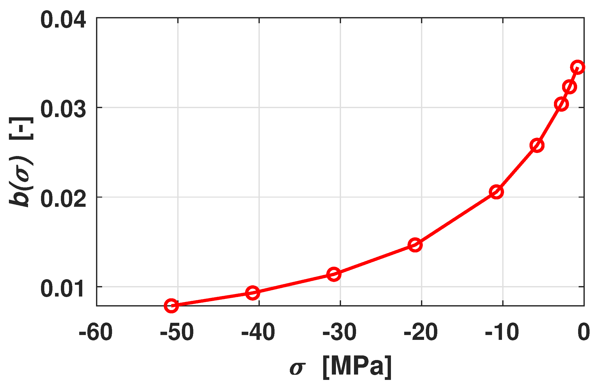
The value of k obtained from minimization is relatively high, but, as described for Galfenol, what is important in the feedback term is that the value of $b\left(\sigma \right)$ remains small. Figure 11 shows how $b\left(\sigma \right)$ depends on $\sigma$, for the k and ${\sigma }_0$ parameters obtained from minimization. It is noticeable that, for increasing compressive stress, the function goes to zero (hyperbolic function of $\sigma$), while it is bounded from above by the value 0.04. From the experimental point of view, the value of ${\sigma }_0=-14$ MPa obtained from minimization procedure can be reasonably interpreted as a pre-stress frozen in the material due to its manufacturing process. Indeed, the Terfenol-D sample under consideration has no stress-annealing [31], while much larger built-in compressive stress of about hundreds of MPa have been reported for SA samples [32].

3.5. Other Criteria

Other techniques to appreciate the similarity between two curves may be considered, such as the minimization of the sum of the ordinates at the same abscissa, i.e.,

$$\min \sum _{i=1}^n{M}_i^{{\sigma }_{min}}-M_i^{{\sigma }_{max}},$$

(21)

where $M_i^{{\sigma }_{min}}$ is the i-th value of the magnetization for the lower stress applied, and $M_i^{{\sigma }_{max}}$ is the i-th value of the magnetization for the higher stress applied, while n is the number of points constituting the variable u. However, this procedure is less effective than the difference of the areas because of the “discretization” introduced by the interpolation on the same abscissa in order to have the average curves from the hysteresis loops. Furthermore, another figure of merit could be the Fréchet distance of two curves, which is defined as the infimum of distances between all reparametrizations of these curves [33]. This latter would be preferable when a set of discrete points are available. In our case, the computation of the area between the curves turns out to be more efficient, since numerical integration algorithms can be directly applied to experimental data.

4. Conclusions

In this paper, the concept of self-similarity for the characteristic curves of the most common magnetostrictive materials has been presented and investigated from the experimental point of view. Three magnetostrictive samples of NSA Galfenol, SA Galfenol, and Terfenol-D have been measured. A reasonable criterion to quantify the self-similarity, based on area differences, has been introduced. Namely, different definitions for the so-called self-similar variable have been adopted with respect to the considered material, and relevant simple expressions between the parameters have been found.